Statistical mechanics of collisionless relaxation in a noninteracting system

Abstract

HMF model, Vlasov equation, Quasi Stationary States We introduce a model of uncoupled pendula, which mimics the dynamical behavior of the Hamiltonian Mean Field (HMF) model. This model has become a paradigm for long-range interactions, like Coulomb or dipolar forces. As in the HMF model, this simplified integrable model is found to obey the Vlasov equation and to exhibit Quasi Stationary States (QSS), which arise after a “collisionless” relaxation process. Both the magnetization and the single particle distribution function in these QSS can be predicted using Lynden-Bell’s theory. The existence of an extra conserved quantity for this model, the energy distribution function, allows us to understand the origin of some discrepancies of the theory with numerical experiments. It also suggests us an improvement of Lynden-Bell’s theory, which we fully implement for the zero field case.

1 Introduction

The long-range character of the interaction is responsible for unusual properties in the thermodynamic and dynamical behaviour in a number of physical situations (Dauxois et al. 2002, Campa et al. 2008, Campa et al. 2009, Dauxois et al. 2009). Systems falling in this class are self-gravitating systems, two-dimensional hydrodynamics, dipolar interacting systems, unscreened plasmas, etc..

We will concentrate in this paper on the study of kinetic equations, which allow one to extrapolate from the single particle to the collective behavior of a physical systems.

Such equations appear also in the study of quantum transport in miniaturised semiconductor devices and nanoscale objects. Indeed, a basic model in this field is provided by the Wigner-Poisson equation (Manfredi, 2001), which recasts quantum dynamics in the classical phase space. The mathematical structure of the Wigner-Poisson system is analogous to that of the Vlasov equation, whose study will be the main topic of this paper.

Two approaches exist for the derivation of kinetic equations, which describe the time evolution of the single particle reduced distribution function $f(\mathbf{r},\mathbf{v},t)$. One can begin with the Liouville equation for the full phase space distribution function (Balescu, 1997). Going through the BBGKY hierarchy and using a perturbative expansion, one can derive the Vlasov, Landau and Lenard-Balescu equations when the perturbative parameter is the strength of the potential. Alternatively, one obtains the Boltzmann equation if one uses density as a perturbation parameter.

A second, more straightforward, approach begins instead with the singular empirical measure in the 6-dimensional single particle phase space and allows one to derive the Vlasov and Lenard-Balescu equations using as perturbation parameter $1/N$, $N$ being the number of particles (Nicholson, 1992). Rigorous mathematical approaches, which began with (Braun et al. 1977, Neunzert 1984), are based on this second approach.

This second approach also emphasizes the role of the mean-field potential, which is crucial when the interaction is long-range. In the $N\to\infty$ limit, the Vlasov equation becomes exact and the evolution towards Boltzmann-Gibbs equilibrium is hindered: the entropy is constant in time. Evolution towards equilibrium appears only if one considers $1/N$ corrections, which leads to “true” kinetic equations, see (Chavanis, 2008) for a review.

Nevertheless, already the Vlasov mean-field term induces an evolution of the single particle distribution function. It was originally observed by (Henon, 1964) that this evolution produces a sort of relaxation and that it preserves some memory of the initial state. Following this remark, (Lynden-Bell, 1967) proposed the concept of “collisionless” or “violent” relaxation, which leads the system towards a Vlasov “equilibrium”. This relaxation occurs in a time of order $O(N^{0})$, whereas later steps of relaxation of the finite $N$ system depend on $N$.

A model which has recently served as a test ground of these theories is the Hamiltonian Mean Field (HMF) model (Antoni & Ruffo, 1995), which describes a system of rotators with all-to-all coupling. The model has been originally introduced with the aim of describing collective phenomena in wave-particle systems of relevance for plasma physics (Elskens & Escande, 2002). Among the applications of interest for this issue, let us quote the one to magnetic layered structures (Campa et al. 2007, Dauxois et al. 2010).

For the HMF model the single particle reduced distribution function $f(\theta,p,t)$ depends on an angle and on the angular momentum. The Vlasov equation is exact for this model in the $N\to\infty$ limit, as was early realized by (Messer & Spohn, 1982). Moreover, the $1/N$ correction to the Vlasov equation, the Lenard-Balescu term, vanishes for one-dimensional models like the HMF model (Bouchet 2004, Bouchet & Dauxois, 2005). This implies that one can expect the system to evolve to equilibrium on time scales larger than $O(N)$. Indeed, it has been found that the system evolves towards Quasi Stationary States (QSS) (Yamaguchi et al. , 2004), which can be interpreted as stable stationary solutions of the Vlasov equation and whose lifetime increases as $N^{1.7}$ for homogeneous states. Since the lifetime of QSS diverges with $N$, we expect that a QSS will last forever in the thermodynamic limit.

QSS have been interpreted as being states that maximize Lynden-Bell entropy (Lynden-Bell, 1967). Quite interestingly, it has been found theoretically, and verified numerically, that, depending on the features of the initial state, one can relax to either homogeneous or inhomogeneous QSS and that this different evolution can be interpreted as a phase-transition (Chavanis 2006, Antoniazzi et al. 2007$a$,$b$).

Lynden-Bell’s approach has been recently successfully applied to the free-electron laser (Barré et al. 2004, Curbis et al. 2007, de Buyl et al. 2009), to the one-dimensional self-gravitating sheet model (Yamaguchi 2008, Levin et al. 2008$b$) to two-dimensional self-gravitating systems (Teles et al. , 2010) and to models of non-neutral plasmas (Levin et al. 2008$a$).

The theory however predicts only regimes in which all macroscopic quantities are exactly constant in time (stationary regimes) and in which the distribution function is a function of the energy alone. This limitation, originating from the very same statistical nature of the theory, causes failures whenever oscillations, non-monotonous energy distribution or clustering regimes are present.

Several attempts have been made to give more firm grounds to Lynden-Bell theory through a careful analysis of the self-consistent interaction present in the Vlasov equation and of the complex relaxation phenomenon it is responsible for. Mostly, the analysis has been performed in the context of 1D self-gravitating systems (Severne & Luwel 1986, Funato et al. 1992, Yamashiro et al. 1992, Tsuchiya et al. 1994). More recently, a description of Vlasov equilibria in a constant mean-field potential has been also introduced (Pomeau, 2008).

We study in this paper the Vlasov equation for a set of uncoupled pendula and we extend Lynden-Bell’s theory to this situation. The model we study should mimic the behavior of the HMF model when this latter has reached a steady state. Since there is no coupling among the pendula, the Vlasov self-consistent potential reduces to a constant potential and collisionless relaxation takes place in the absence of variations of the potential.

In spite of all these simplifications, many of the effects found in the HMF model are still present and are still well reproduced by the theory. In particular, the theory predicts the value of the magnetization attained by the system in the QSS and the occurrence of a phase transition from a homogeneous (zero magnetization) QSS to an inhomogeneous (magnetized) one. For our simple integrable system, it’s also easy to understand how to improve the theory by adding conservation laws. We here propose to add conservation of moments of the velocity distribution in the case of homogeneous states.

The paper is organized as follows. In Section 2 we introduce the Vlasov equation for the system of uncoupled pendula. In Section 3 we present some numerical simulations showing the presence of homogeneous and inhomogeneous states. The following Section 4 is devoted to the development of Lynden-Bell’s theory, which is then successfully compared with numerical experiments in Section 5. Section 6 discusses some possible improvements of the theory, which includes an extra conservation law and Section 7 presents some conclusions.

2 Uncoupled pendula and HMF model

We consider the following Hamiltonian, describing a system of $N$ uncoupled pendula,

$$H=\sum_{j=1}^{N}\frac{p_{j}^{2}}{2}-\mathcal{H}\sum_{j=1}^{N}\cos\theta_{j}~{},$$ (1)

where $\theta_{j}$ is the angle of the $j$-th pendulum and $p_{j}$ the corresponding angular momentum. The external field $\mathcal{H}$ represents the action of gravity.

Model (1) is intended to mimic, in the large $N$ limit, the dynamics of the HMF model (Antoni & Ruffo, 1995), whose Hamiltonian is

$$H_{HMF}=\sum_{j=1}^{N}\frac{p_{j}^{2}}{2}-\frac{1}{2N}\sum_{i,j=1}^{N}\cos(\theta_{i}-\theta_{j}).$$ (2)

The rationale for this comparison is that, if one introduces the magnetization

$$\mathbf{m}=\frac{1}{N}\sum_{j=1}^{N}\left(\cos\theta_{j},\sin\theta_{j}\right)=\left(m_{x},m_{y}\right)=m\left(\cos\phi,\sin\phi\right)~{},$$ (3)

one can rewrite the potential of the HMF model as $-Nm^{2}/2$, while the one of model (1) reads $-N\mathcal{H}m_{x}$. It is then evident that the two potentials have the same form if one identifies $\mathcal{H}$ with $m_{x}/2$ and one disregards the motion of the phase of the magnetization, i.e. one sets $\phi=0$ ($m=m_{x}$), which can always be done without loss of generality taking the rotational invariance of Hamiltonian (2) into account. From now on, we will then identify the magnetization $m$ with $m_{x}$. The value of $m$ detects the “homogeneity” of the system: $m=0$ implies that the system is homogeneous while $m>0$ indicates an inhomogeneous system. This terminology corresponds to a particle representation of both system (1) and (2), according to which, to each pendulum we associate a particle moving on a circle. Then, $m=1$ means that all particles are located at $\theta=0$, and therefore the particles are fully clustered, while when $m=0$ the particles are homogeneously dispersed on the circle. In the following, we will make use of $m$ to quantify the state of the system and track its evolution in time.

We will not present in this paper results for the finite $N$ case. We will instead consider the time evolution of the single particle reduced distribution function $f(\theta,p,t)$, which obeys the Vlasov equation

$$\frac{\partial f}{\partial t}+\{f,h\}=0~{},$$ (4)

where $\{\cdot,\cdot\}$ are Poisson brackets and $h$ is the single particle Hamiltonian, which, for model (1) is given by

$$h(\theta,p)=\frac{p^{2}}{2}-\mathcal{H}\cos\theta~{},$$ (5)

while for the HMF model (2) is

$$h_{HMF}(\theta,p)=\frac{p^{2}}{2}-m_{x}[f]\cos\theta-m_{y}[f]\sin\theta,$$ (6)

where

$$m_{x}[f] = \int d\theta dp\cos\theta f(\theta,p,t)$$ (7)

$$m_{y}[f] = \int d\theta dp\sin\theta f(\theta,p,t)~{}.$$ (8)

The main difference between the two single particle Hamiltonians is that the one of model (1) does not depend on $f$, it is simply a function of the phase space variables. The relation between the two models is here even more evident, it amounts to identify $m_{x}[f]$ with $\mathcal{H}$ and to put $m_{y}[f]=0$ (the factor 1/2 present in the previous identification was due to the presence of pair interactions in the potential). The absence of any dependence on $f$ in the single particle Hamiltonian makes a big difference. Physically, it means that each particle moves on a constant energy trajectory in an external potential which is fixed. This does not mean that $f$ does not evolve in time, and therefore we expect also in this case a “collisionless” relaxation. The questions we explore in this paper are how well Lynden-Bell’s theory represents this relaxation and how close it is to the one of the HMF model. A crucial aspect of the relaxation of the uncoupled pendula model is the conservation of the following energy distribution

$$p(e)=\int d\theta\ dp\ f(\theta,p,0)\delta(e-h(\theta,p))~{},$$ (9)

which remains constant in time, as fixed by the initial value of $f$. Lynden-Bell’s theory does not take this extra conservation law into account: we will try in Section 6 to implement in the theory this aspect for homogeneous states.

3 Numerical results: homogeneous vs. inhomogeneous states

We have solved the Vlasov equation (4) for the uncoupled pendula via a semi-Lagrangian method coupled to cubic splines. This method is based on a representation of $f$ on a grid, i.e. $f_{i,j}=f(\theta_{i},p_{j})$ at the grid points $\{(\theta_{i},p_{j});i\in[1:N_{\theta}];j\in[1:N_{p}]\}$. We refer the reader to (Sonnendrücker et al. 1999) for the semi-Lagrangian method, or (de Buyl, 2010) for details regarding mean-field models. The relevant parameters for these simulations are: $N_{\theta}$, the number of grid points in the $\theta$-direction, $N_{p}$ the number of grid points in the $p$-direction, $\Delta t$, the time-step and $p_{max}$, which defines the size of the simulation box in phase space as $[-\pi:\pi]\times[-p_{max}:p_{max}]$. We use in all simulations reported in this paper the following values: $N_{\theta}=N_{p}=256$, $p_{max}=-p_{min}=2.5$ and $\Delta t=0.1$.

We consider a “waterbag” initial condition: the particles, or phase space fluid elements, occupy a rectangular region of phase space characterized by a half width $\Delta\theta$ in angle and $\Delta p$ in momentum

$$\left\{\begin{array}[]{l l l}f(\theta,p,0)&=&f_{0}\textrm{ if }|\theta|\leq\Delta\theta\textrm{ and }|p|\leq\Delta{}p\cr&=&0\textrm{ , else.}\cr&&f_{0}=\left(4\Delta\theta\Delta p\right)^{-1}\end{array}\right.$$ (10)

Using this initial condition, magnetization at time zero and energy per particle are given by $m_{0}=\frac{\sin\Delta\theta}{\Delta\theta}$ and $U=lim_{N\to\infty}H/N=\frac{\Delta p^{2}}{6}-\mathcal{H}m_{0}$, respectively. While the magnetization evolves in time, the energy is a conserved quantity. Since the Vlasov equation is a Liouville equation for $f$, the evolution of the waterbag initial condition is such that the region occupied by the “fluid level” $f_{0}$ deforms but conserves its area in phase space. Two qualitatively different regimes take place depending on whether $\mathcal{H}$ is equal to $0$ or not. We represent the evolution of the waterbag initial condition by the Vlasov dynamics in Fig. 1, plotting the contour line of the region occupied by the level $f_{0}$ in phase space at different times. The time evolution of $m$ is shown in Fig. 2.

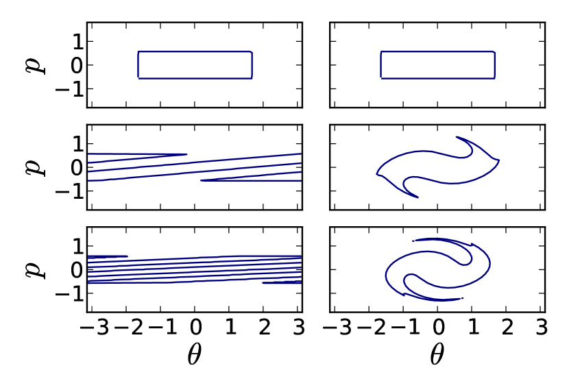
Figure 1: Evolution of the waterbag initial condition (10) with $\Delta\theta=1.66$ and $\Delta p=0.57$. We plot the contour lines of the region occupied by the “fluid level” $f_{0}$ in phase space with time increasing from top to bottom. The left column represents the case $\mathcal{H}=0$ and in the right column $\mathcal{H}=0.75$.

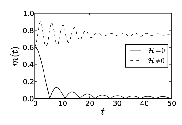
Figure 2: Magnetization $m$ vs. time for the same conditions of Fig. 1.

In the free-streaming case ($\mathcal{H}=0$), the magnetization $m$ relaxes asymptotically to zero. Correspondingly, the initial waterbag spreads over the whole $[-\pi:\pi]$ interval. In the $\mathcal{H}\neq 0$ case, a finite value of $m$ is attained at long times, with the fluid forming a clump around $\theta=0$. This reflects the different evolutions towards either a homogeneous state with $m=0$ or towards an inhomogeneous state with $m\neq 0$.

4 Lynden-Bell’s theory

Lynden-Bell’s theory (Lynden-Bell, 1967) aims at predicting asymptotic states of the Vlasov dynamics. The theory allows one to compute analytically $\bar{f}(\theta,p)$, the coarse grained single particle distribution function. Lynden-Bell’s entropy is derived by a combinatorial counting of the allowed states in a phase space cell. We write here the expression of the entropy as applicable to the waterbag initial condition in formula (10)

$$s(\bar{f})=-\int dp\ d\theta\ \left[\frac{\bar{f}}{f_{0}}\ln\frac{\bar{f}}{f_{0}}+\left(1-\frac{\bar{f}}{f_{0}}\right)\ln\left(1-\frac{\bar{f}}{f_{0}}\right)\right]\textrm{ . }$$ (11)

Under the constraints of “mass”, $\int fd\theta dp$, and energy conservation, the maximization of entropy (11) for the waterbag initial condition (10) leads to the following steady state distribution

$$\bar{f}(\theta,p)=\frac{f_{0}}{e^{\beta(p^{2}/2-\mathcal{H}\cos\theta)+\mu}+1}~{},$$ (12)

where $\mu$ and $\beta$ are Lagrange multipliers associated respectively to mass and energy conservation. They can be obtained, together with $m_{QSS}$, the magnetization in the QSS, by solving the following set of equations

$$\frac{f_{0}x}{\sqrt{\beta}}\int d\theta\ e^{\beta\mathcal{H}\cos\theta}F_{0}(xe^{\beta\mathcal{H}\cos\theta})=1$$ (13)

$$\frac{f_{0}x}{2\beta^{2/3}}\int d\theta\ e^{\beta\mathcal{H}\cos\theta}F_{2}(xe^{\beta\mathcal{H}\cos\theta})-\mathcal{H}m_{QSS}=U$$ (14)

$$\frac{f_{0}x}{\sqrt{\beta}}\int d\theta\ \cos\theta\ e^{\beta\mathcal{H}\cos\theta}F_{0}(xe^{\beta\mathcal{H}\cos\theta})=m_{QSS}$$ (15)

where $x=e^{-\mu}$ and the $F_{n}$ are defined as

$$F_{n}(x)=\int dv\ \frac{v^{n}}{e^{v^{2}/2}+x}~{}.$$ (16)

We have solved the system of equations (13) using the Newton-Raphson method (Press et al. , 1996).

In the context of the uncoupled pendula model we are thus free to choose three parameters: $\Delta\theta$, $\Delta p$ and $\mathcal{H}$. If we want to compare the behavior of this model with the HMF model, we have to reduce the free parameters to two. A physically reasonable restriction is to impose the self-consistency condition

$$m_{QSS}=\mathcal{H}~{}.$$ (17)

Then, once $\Delta\theta$ and $\Delta p$ are given, system (13) allows to solve for $m_{QSS}$, $\beta$ and $\mu$ (taking into account that $U$ can be written in terms of $\Delta\theta$, $\Delta p$ and $m_{QSS}$), which substituted in turn into (12) (with $\mathcal{H}=m_{QSS}$) allows us to obtain the single particle distribution function in the QSS.

5 Comparing with simulations

The predicted value of $m_{QSS}$ offers a straightforward way to compare the result of Lynden-Bell’s theory with simulations. In Fig. 3 we plot $m_{QSS}$ vs. $\Delta p$ for $\Delta\theta=1.66$ for both theory and numerical experiment.

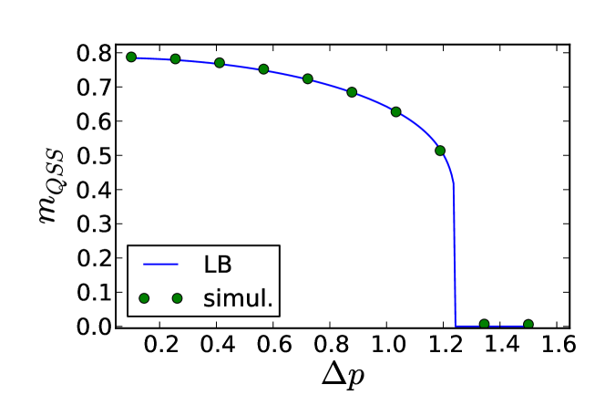
Figure 3: Comparison of the magnetization in the QSS, $m_{QSS}$, as predicted by Lynden-Bell’s theory with the one resulting from the simulations, for a waterbag initial condition (10) characterized by $\Delta\theta=1.66$.

The agreement in all the explored range of $\Delta p$ is quite satisfactory.

A comment is however in order: if the self-consistent criterion is fulfilled with $\mathcal{H}=m_{QSS}=0$, $m_{QSS}$ converges exactly to $0$ in the simulations. This comes from the fact that the force term $-\partial h(\theta,p)/\partial\theta$ in the Vlasov equation vanishes and then the initial waterbag evolves under free streaming, leading necessarily to a homogeneous distribution with respect to $\theta$ (see the left column of Fig1). The fact that we find an agreement also in the region where $\mathcal{H}\neq 0$ is less trivial.

In order to explore with a finer detail the agreement of theory with numerical experiments, we proceed to the comparison of the single particle distribution function in the QSS. To this aim, we define the marginal distributions

$$\varphi(p)=\int d\theta\ f(\theta,p)\quad\mathrm{;}\quad\rho(\theta)=\int dp\ f(\theta,p)~{}.$$ (18)

In Fig. 4 we display the marginal $\varphi(p)$ for $\Delta\theta=1.66$ and for various values of $\Delta p$ and in Fig. 5 the marginal $\rho(\theta)$ for the same values of $\Delta\theta$ and $\Delta p$.

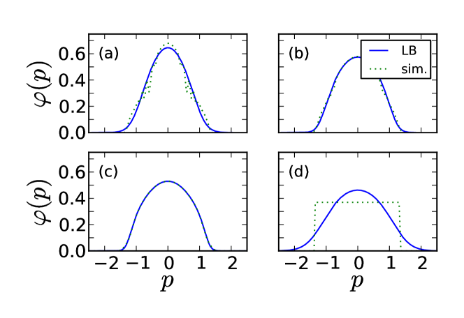
Figure 4: The marginal $\varphi(p)$ for $\Delta\theta=1.66$ and $\Delta p=0.41(a)$,$0.72(b)$, $1.03(c)$ and $1.34(d)$.

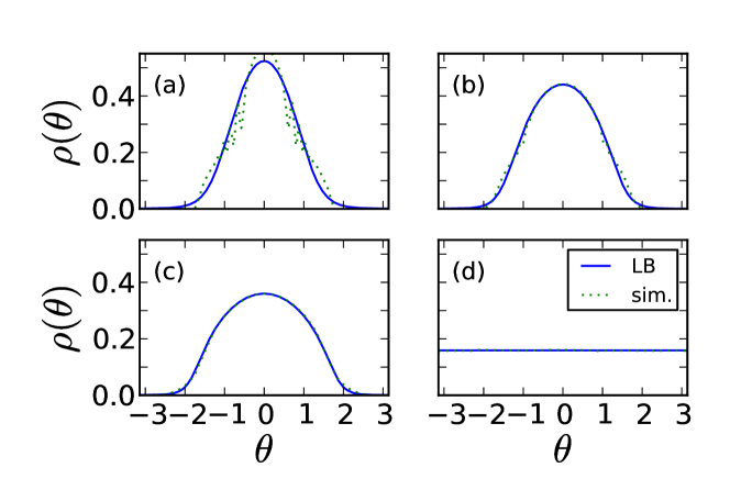
Figure 5: The marginal $\rho(\theta)$ for the same values of $\Delta\theta$ and $\Delta p$ as in Fig. 4

Apart from a disagreement at small scales, which is expected due to the filamentary structure of $f$ shown in Fig. 1 (Lynden-Bell’s theory provides a prediction for the coarse-grained distribution $\bar{f}$), the comparison in panels $(a)$, $(b)$ and $(c)$ of Figs. 4 and 5 is quite good. Lynden-Bell’s theory catches some basic aspects of the spreading of the distribution along constant energy levels induced by the Vlasov equation. However, a major drawback of the theory appears in panel $(d)$: while the marginal $\rho(\theta)$ is correctly predicted, $\varphi(p)$ disagrees with numerical simulations. This negative result is nevertheless somewhat expected, because the time evolution with $\mathcal{H}=0$ is a free streaming: each momentum level is conserved by the dynamics. This latter aspect is not at all taken into account by the theory, which therefore fails to reproduce $\varphi(p)$.

We have checked the predictions of the theory for a specific value of $\Delta\theta$: we cannot expect them to be reliable for all values of $\Delta\theta$. Indeed, the predictions of $m_{QSS}$ shown in Fig. 6 for $\Delta\theta=\pi$ are worse, although the transition value of $\Delta p$ is well reproduced.

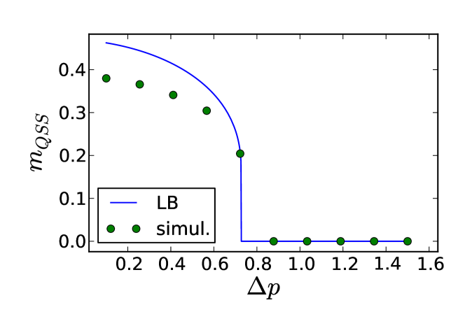
Figure 6: Comparison of the magnetization $m_{QSS}$ as predicted by Lynden-Bell’s theory with the one resulting from the simulations. We take here $\Delta\theta=\pi$.

Since the source of disagreement, as we have observed above, can be in the failure of the theory to take into account extra conservation laws, we compare in Fig. 7, the energy distribution (9) predicted by the theory with the one resulting from the numerics (this latter being constant in time and fully determined by the initial condition). As expected, when the value of $m_{QSS}$ is better predicted (e.g. for $\Delta\theta=\pi$ and $\Delta p=0.72$), the energy distribution found using Lynden-Bell’s theory is closer to the initial one.

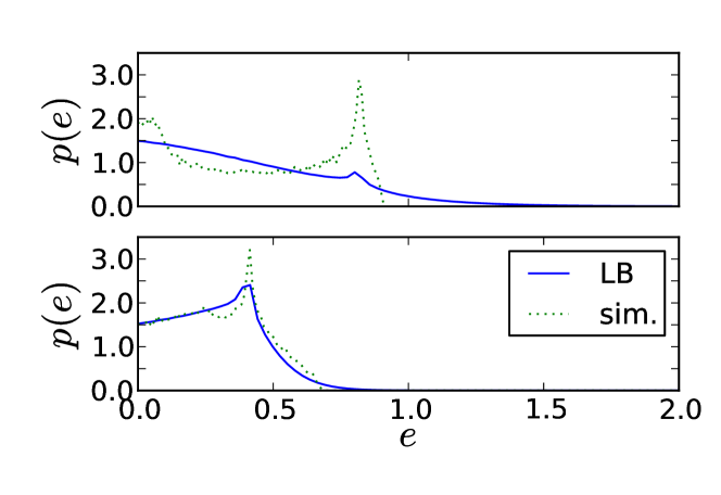
Figure 7: Energy distributions $p(e)$ given by formula (9) for $\Delta\theta=\pi$, $\Delta p=0.41$ (top panel) and $\Delta\theta=\pi$, $\Delta p=0.72$ (bottom panel), computed using Lynden-Bell’s theory and numerically.

We therefore argue that the success of Lynden-Bell’s theory in the case of uncoupled pendula originates partly from the fact that the initial energy distribution $p(e)$ is close enough to the one predicted by Lynden-Bell’s theory itself. This may look accidental and throw some doubts on the general validity of the theory. However, the excellent agreement found for $\Delta\theta=1.66$ remains a good indication of the quality of the predictions of the theory. Further systematic work of comparison of the theory with numerical experiment is required in order to assess the origin of disagreements.

6 Adding conserved quantities in the zero field case

The failure of Lynden-Bell’s theory to reproduce $\varphi(p)$ for the homogeneous case ($\mathcal{H}=0$) could be easily understood because of the trivial dynamics involved. A deeper remark is that the conservation of the energy distribution $p(e)$ reduces for $\mathcal{H}=0$ to the conservation of $\varphi(p)$. We here then impose this constraint by requiring the conservation of the even moments of $\varphi(p)$

$$P_{2n}[f]=\int d\theta\ dp\ f(\theta,p)p^{2n}\quad\quad n=1,2,\dots~{},$$ (19)

which is a consequence of the conservation of each individual momentum for the uncoupled pendula with $\mathcal{H}=0$. The odd moments are all zero for symmetry reasons. The $n=0$ moment is the total “mass” and its conservation is already imposed in the Lynden-Bell’s theory. The $n=1$ moment is the energy and has already been considered: we denote the corresponding theory by LB1. We restrict here to impose the extra conservation of the $n=2$ and $n=3$ moments: the corresponding theories will be denoted as LB2 and LB3.

Maximizing Lynden-Bell’s entropy (11) leads to the following coarse grained distribution function

$$\bar{f}(\theta,p)=\frac{f_{0}}{e^{\beta p^{2}/2+\sigma_{2}p^{4}+\sigma_{3}p^{6}+\mu}+1}~{},$$ (20)

where $\beta$ is the Lagrange multiplier conjugated to the energy, $\sigma_{2}$ and $\sigma_{3}$ those corresponding to the $n=2$ and $n=3$ moments. The new system of equations to be solved is

$$f_{0}\ x\ 2\pi\ G_{0}(x,\beta,\sigma_{2,3})=1$$ (21a)

$$f_{0}\ x\ \pi\ G_{2}(x,\beta,\sigma_{2,3})=U$$ (21b)

$$f_{0}\ x\ 2\pi\ G_{2n}(x,\beta,\sigma_{2,3})=P_{2n}[f_{|t=0}]\quad\quad n=2,3$$ (21c)

where $G_{2n}(x,\beta,\sigma_{4,6})=\int dv\ v^{2n}(e^{\beta v^{2}/2+\sigma_{2}v^{4}+\sigma_{3}v^{6}}+x)^{-1}$.

We find the result displayed in Fig. 8. The presence of two humps in $\varphi(p)$ for the LB2 theory and three humps for LB3 looks surprising, but it should be interpreted as similar to the Gibbs phenomenon: approximating a function with a limited set of basis functions can give rise to oscillations. Increasing the number of conserved moments of $\varphi(p)$ can only lead to the waterbag distribution, since it is the only one that has the good values of $P_{2n}[f]$ for all $n$’s.

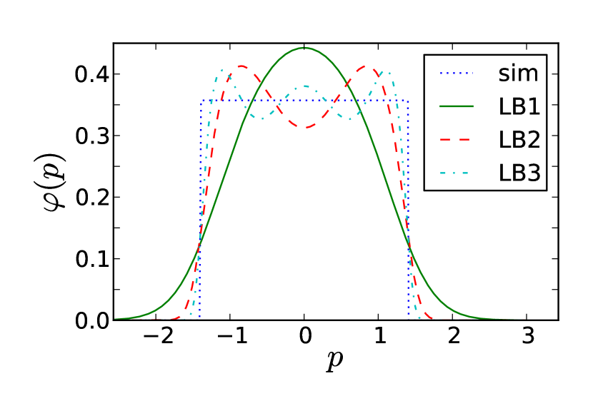
Figure 8: Comparison $\varphi(p)$ obtained from LB1, LB2 and LB3 theories (see text) with the simulation for $\Delta p=1.4$ and $\Delta\theta=1.66$. For the LB3 theory the values of the Lagrange multipliers are: $x=1.29$, $\beta=3.98$, $\sigma_{2}=-14.45$ and $\sigma_{3}=12.30$.

It is worth remarking that, for high values of $\beta$, the LB1 theory is able to reproduce a step profile accurately enough, providing good results for the homogeneous situations considered here (one can compare this limit with the low temperature Fermi distribution). Our extension to the LB2 and LB3 theories allows us to obtain a better match in all situations where $\beta$ is smaller, as illustrated in Fig. 8. Indeed, lower values of $\Delta\theta$ (at constant $\Delta p$) favour smaller values of $\beta$. On the other hand, one can prove, by a direct inspection of Eqs.21, that, at fixed $\Delta\theta$, $\beta$ scales as $\Delta p^{-2}$ and $\sigma_{n}$ as $\Delta p^{-2n}$.

Let us mention that, although computationally more complex, one could in principle obtain improved theories in the $\mathcal{H}\neq 0$ case by imposing the conservation of the moments of the energy distribution $p(e)$. For the HMF model this approach is unfortunately not viable because $p(e)$ is not conserved.

7 Conclusions

With the aim of reaching a deeper understanding of the Quasi Stationary States (QSS) observed in the HMF model, we have studied in this paper the Vlasov equation of a set of uncoupled pendula.

These studies are relevant for understanding the extrapolation from single particle to collective properties in physical systems with unscreened long-range interactions, like Coulomb or dipolar. They will also lead to a better understanding of kinetic equations, like the Vlasov equation, whose mathematical structure appears in many different fields, including quantum transport at the nanoscale with the use of the Wigner-Poisson system.

Lynden-Bell’s theory applies successfully to the uncoupled pendula model. We have found good predictions for both the magnetization and the marginals $\varphi(p)$ and $\rho(\theta)$ of the single particle distribution function in the QSS, although the agreement with numerical simulations depends on the chosen initial state.

The discrepancy that we observe between the theory and the numerical results has provided us with a hint on how to extend the theory by including the moments of the velocity distribution for the zero field case. This is justified by the presence of a further conserved quantity for the uncoupled pendula case: the energy distribution $p(e)$ in formula (9).

Unfortunately this approach is not straightforwardly applicable to the HMF, because the energy distribution is not conserved. However, it has been recently realized that the steady state distribution of the model of uncoupled pendula can be obtained analytically (de Buyl et al. , 2010) and shows properties very similar to those of the HMF model.

- [1]
- [2] Antoni, M. & Ruffo, S. 1995 Clustering and relaxation in Hamiltonian long-range dynamics. Phys. Rev. E 52, 2361–2374.
- [3]
- [4] Antoniazzi, A., Fanelli, D., Ruffo, S. & Yamaguchi, Y. Y. 2007 Nonequilibrium tricritical point in a system with long-range interactions. Phys. Rev. Lett. 99, 040601.
- [5]
- [6] Antoniazzi, A., Fanelli, D., Barré, J., Chavanis, P.-H., Dauxois, T. & Ruffo, S. 2007 Maximum entropy principle explains quasistationary states in systems with long-range interactions: The example of the Hamiltonian mean-field model. Phys. Rev. E 75, 011112.
- [7]
- [8] Balescu, R. 1997 Statistical Dynamics - Matter out of Equilibrium. London: Imperial College Press.
- [9]
- [10] Barré, J., Dauxois, T., De Ninno, G., Fanelli, D. & Ruffo, S. 2004 Statistical theory of high-gain free-electron laser saturation. Phys. Rev. E 69, 045501(R).
- [11]
- [12] Bouchet, F. 2004 Stochastic process of equilibrium fluctuations of a system with long-range interactions. Physical Review E 70, 036113.
- [13]
- [14] Bouchet, F. & Dauxois T. 2005 Prediction of anomalous diffusion and algebraic relaxations for long-range interacting systems, using classical statistical mechanics. Physical Review E 72, 045103(R).
- [15]
- [16] Braun, W. & Hepp K., 1977 The Vlasov dynamics and its fluctuations in the limit of interacting classical particles. Comm. Math. Phys. 56, 101–113.
- [17]
- [18] Campa, A., Giansanti, A., Morigi, G. & Sylos Labini, F. (eds) 2008 Dynamics and Thermodynamics of Systems with Long Range Interactions: Theory and Experiments, AIP Conference Proceedings, 970.
- [19]
- [20] Campa, A., Khomeriki, R., Mukamel, D. & Ruffo, S. 2007 Long-range effects in layered spin structure. Phys. Rev. B 76 064415.
- [21]
- [22] Campa, A., Dauxois, T. & Ruffo, S. 2009 Statistical mechanics and dynamics of solvable models with long-range interactions. Phys. Rep. 480, 57–159.
- [23]
- [24] Chavanis, P. H. 2006 Lynden-Bell and Tsallis distributions for the HMF model. European Physical Journal B 53, 487–501.
- [25]
- [26] Chavanis, P. H. 2008 Dynamics and thermodynamics of systems with long-range interactions: interpretation of the different functionals. in (Campa et al. 2008).
- [27]
- [28] Curbis, F., Antoniazzi, A., De Ninno, G. & Fanelli, D. 2007 Maximum entropy principle and coherent harmonic generation using a single-pass free-electron laser. Eur. Phys. J. B 59, 527–533.
- [29]
- [30] Dauxois, T., Ruffo, S., Arimondo, E. & Wilkens, M. (eds) 2002 Dynamics and Thermodynamics of Systems With Long Range Interactions, volume 602 of Lecture Notes in Physics Springer-Verlag.
- [31]
- [32] Dauxois, T., Ruffo, S. & Cugliandolo, L. 2009 Long range interacting systems, Les Houches Summer School 2008. Oxford: Oxford University Press.
- [33]
- [34] Dauxois, T., de Buyl, P., Lori, L. & Ruffo 2010, S. Models with short and long-range interactions: phase diagram and re-entrant phase. J. Stat. Mech.: Theory and Experiment, submitted.
- [35]
- [36] Elskens, Y. & Escande, D. 2002 , Microscopic Dynamics of Plasmas and Chaos, Bristol: IOP Publishing, Bristol (2002).
- [37]
- [38] de Buyl, P., Fanelli, D., Bachelard, R. & De Ninno, G. 2009 Out-of-equilibrium mean-field dynamics of a model for wave-particle interaction. Phys. Rev. ST Accel. Beams 12, 060704.
- [39]
- [40] de Buyl, P. 2010 Numerical resolution of the Vlasov equation for the Hamiltonian Mean-Field model. Commun. Nonlinear. Sci. Numer. Simulat. 15, 2133–2139.
- [41]
- [42] de Buyl, P., Mukamel, D., & Ruffo, S. 2010 in preparation.
- [43]
- [44] Funato, Y., Makino, J. & Ebisuzaki, T. 1992 Violent relaxation is not a relaxation process. Publ. Astron. Soc. Japan 44, 613–621.
- [45]
- [46] Hénon, M. 1964 L’évolution initiale d’un amas sphérique. Annales d’Astrophysique 27, 83–91.
- [47]
- [48] Levin, Y., Pakter, R. & Rizzato, F. B. 2008 Collisionless relaxation in gravitational systems: From violent relaxation to gravothermal collapse. Phys. Rev. E 78, 021130.
- [49]
- [50] Levin, Y., Pakter, R. & Teles, T. N. 2008 Collisionless relaxation in non-neutral plasmas. Phys. Rev. Lett. 100, 040604.
- [51]
- [52] Lynden-Bell, D. 1967 Statistical mechanics of violent relaxation in stellar systems. Mont. Not. R. Astron. Soc. 136, 101–121.
- [53]
- [54] Manfredi G. 2001 Self-consistent fluid model for a quantum electron gas. Phys. Rev. B 64 075316.
- [55]
- [56] Messer, J. & Spohn, H. 1982 Statistical mechanics of the isothermal Lane-Emden equation. J. Stat. Phys. 29, 561–578.
- [57]
- [58] Neunzert H. 1984 An introduction to the nonlinear Boltzmann-Vlasov equation. in C. Cercignani Ed.: Kinetic Theories and the Boltzmann Equation, Lect. Notes in Math. 1048, 60–71.
- [59]
- [60] Nicholson, D. R. 1992 Introduction to Plasma Physics, Krieger Pub. Co..
- [61]
- [62] Pomeau, Y. 2008 Statistical mechanics of gravitational plasmas. Second Warsaw School of Statistical Physics.
- [63]
- [64] Severne, G. & Luwel, M. 1986 Violent relaxation and mixing in non-uniform one-dimensional gravitational systems. Astrophys. Space Sci. 122, 299–325.
- [65]
- [66] Teles T. N., Levin Y., Pakter R. & Rizzato F. B. 2010 Statistical mechanics of unbound two dimensional self-gravitating systems. arXiv:1004.0247.
- [67]
- [68] Tsuchiya, T., Konishi, T. & Gouda N. 1994 Quasiequilibria in one-dimensional self-gravitating many-body systems. Phys. Rev. E 50, 2607–2615.
- [69]
- [70] Yamaguchi, Y. Y. 2008 One-dimensional self-gravitating sheet model and Lynden-Bell statistics. Phys. Rev. E 78, 041114.
- [71]
- [72] Yamaguchi, Y. Y., Barré, J., Bouchet, F., Dauxois, T. & Ruffo, S. 2004 Stability criteria of the Vlasov equation and quasi-stationary states of the HMF model. Physica A 337, 36–66.
- [73]
- [74] Yamashiro, T., Gouda, N. & Sakagami, N. 1992 Origin of core-halo structure in one-dimensional self-gravitating system. Prog. Theor. Phys. 88, 269–282.
- [75]