Alpha Shape Topology of the Cosmic Web

Abstract

We study the topology of the Megaparsec Cosmic Web on the basis of the Alpha Shapes of the galaxy distribution. The simplicial complexes of the alpha shapes are used to determine the set of Betti numbers ($\beta_{\rm k},k=1,\ldots,D$), which represent a complete characterization of the topology of a manifold. This forms a useful extension of the geometry and topology of the galaxy distribution by Minkowski functionals, of which three specify the geometrical structure of surfaces and one, the Euler characteristic, represents a key aspect of its topology. In order to develop an intuitive understanding for the relation between Betti numbers and the running $\alpha$ parameter of the alpha shapes, and thus in how far they may discriminate between different topologies, we study them within the context of simple heuristic Voronoi clustering models. These may be tuned to consist of a few or even only one specific morphological element of the Cosmic Web, ie. clusters, filaments or sheets.

I Introduction: the Cosmic Web

The large scale distribution of matter revealed by galaxy surveys features a complex network of interconnected filamentary galaxy associations. This network, which has become known as the Cosmic Web [1], contains structures from a few megaparsecs up to tens and even hundreds of Megaparsecs of size. Galaxies and mass exist in a wispy weblike spatial arrangement consisting of dense compact clusters, elongated filaments, and sheetlike walls, amidst large near-empty void regions, with similar patterns existing at earlier epochs, albeit over smaller scales. The hierarchical nature of this mass distribution, marked by substructure over a wide range of scales and densities, has been clearly demonstrated [2]. Its appearance has been most dramatically illustrated by the recently produced maps of the nearby cosmos, the 2dFGRS, the SDSS and the 2MASS redshift surveys [3, 4, 5].

The vast Megaparsec cosmic web is one of the most striking examples of complex geometric patterns found in nature, and certainly the largest in terms of sheer size. Computer simulations suggest that the observed cellular patterns are a prominent and natural aspect of cosmic structure formation through gravitational instability [6], the standard paradigm for the emergence of structure in our Universe [7, 8].

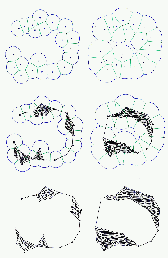
Figure 1: Illustration of Alpha Shapes. For two different values of $\alpha$, the figure shows the relation between the 2-D point distribution, the value of $\alpha$ and the resulting alpha shape. Around each point in the point sample, circles of radius $R^{2}=\alpha$ are drawn. The outline of the corresponding Voronoi tessellation within the space covered by the circles is indicated by the edges (top). All Delaunay simplices - vertices, edges and cells - entirely located within this space are shown in black (centre). The final resulting alpha shape is shown in the bottom panel. Left: small $\alpha$ value. Right: large $\alpha$ value. Based on transparencies of H. Edelsbrunner, used at the Jigsaw conference, Leiden, 2006.

I-A Web Analysis

Despite the multitude of elaborate qualitative descriptions it has remained a major challenge to characterize the structure, geometry and topology of the Cosmic Web. Many attempts to describe, let alone identify, the features and components of the Cosmic Web have been of a rather heuristic nature. The overwhelming complexity of both the individual structures as well as their connectivity, the lack of structural symmetries, its intrinsic multiscale nature and the wide range of densities that one finds in the cosmic matter distribution has prevented the use of simple and straightforward instruments.

In the observational reality galaxies are the main tracers of the cosmic web and it is mainly through the measurement of the redshift distribution of galaxies that we have been able to map its structure. Likewise, simulations of the evolving cosmic matter distribution are almost exclusively based upon N-body particle computer calculations, involving a discrete representation of the features we seek to study. Both the galaxy distribution as well as the particles in an N-body simulation are examples of spatial point processes in that they are discretely sampled and have an irregular spatial distribution.

Topology of the Cosmic Density Field
For furthering our understanding of the Cosmic Web, and to investigate its structure and dynamics, it is of prime importance to have access to a set of proper and objective analysis tools. In this contribution we address the topological and morphological analysis of the large scale galaxy distribution. To this end, we focus in particular on the alpha shapes of the galaxy distribution, one of the principal concepts from the field of Computational Topology [9].

In numerous previous studies, the topology and geometry of the cosmic matter distribution have been adressed in a variety of ways. A direct probe of the shape of the local matter distribution is the statistical distribution of inertial moments [10, 11, 12]. These concepts are closely related to the full characterization of the local geometry of the matter distribution in terms of four Minkowski functionals [13, 14]. These are the volume, surface area, integrated mean curvature and Euler characteristic of the enclosed density surfaces. The Minkowski functionals are solidly based in the theory of spatial statistics and also have the great advantage of being known analytically in the case of Gaussian random fields. In particular, the Euler characteristic or the closely related genus of the density field has received substantial attention as a strongly discriminating factor between intrinsically different spatial patterns [15, 16].

The Minkowski functionals provide global characterisations of structure. An attempt to extend its scope towards providing locally defined topological measures of the density field has been developed in the SURFGEN project defined by Sahni and Shandarin and their coworkers [17, 18]. It involves a local topology characterization in terms of Shapefinders, the ratios of Minkowski functionals. The main problem remains the user-defined, and thus potentially biased, nature of the continuous density field inferred from the sample of discrete objects. The usual filtering techniques suppress substructure on a scale smaller than the filter radius, introduce artificial topological features in sparsely sampled regions and diminish the flattened or elongated morphology of the spatial patterns. Quite possibly the introduction of more advanced geometry based methods to trace the density field may prove a major advance towards solving this problem (see contribution by Aragón-Calvo & Shandarin in this volume). Martinez [19] and Saar [20] have generalized the use of Minkowski Functionals by calculating their values in a hierarchy of scales generated from wavelet-smoothed volume limited subsamples of the 2dF catalogue. This approach is particularly effective in dealing with non-Gaussian point distributions since the smoothing is not predicated on the use of Gaussian smoothing kernels.

Alpha Shapes
While most of the above topological techniques depend on some sort of user-specific smoothing and related threshold to specify surfaces of which the topology may be determined. An alternative philosophy is to try to let the point or galaxy distribution define its own natural surfaces. This is precisely where Alpha Shapes enter the stage.

Alpha Shapes may be invoked to compute a large variety of geometrical and topological measures of a point distribution. Here we focus in particular on the determination of the Betti numbers to characterize the topology of the weblike spatial patterns sampled by a discrete point - i.e. galaxy - distribution. In essence, the Betti numbers $\beta_{k}$ counts the number of k-dimensional holes in an alpha complex. The first three Betti numbers, whose behaviour we will assess here, specify the number of individual complex ($\beta_{0}$), the number of independent tunnels ($\beta_{1}$) and the number of enclosed voids ($\beta_{2}$). Betti numbers contain more detailed topological information than Minkowski functionals, but unlike the latter are not sensitive to the actual geometry of an alpha shape. In order to build up an intuitive understanding of the behaviour of Betti numbers with respect to the weblike configurations encountered in the Megaparsec Universe, or in simulations of its formation, we here present a study of simpler heuristic Voronoi clustering models. On the basis of their topological simplicity we seek to connect the behaviour of Betti numbers to distinct morphological elements of the large scale Universe, such as filaments, walls, clusters and voids.

II Alpha Shapes

Alpha Shape is a description of the (intuitive) notion of the shape of a discrete point set. Alpha Shapes of a discrete point distribution are subsets of a Delaunay triangulation and were introduced by Edelsbrunner and collaborators [9, 21, 22, 23] (for a recent review see [24], and the excellent book by Edelsbrunner & Harer 2010 [25] for a thorough introduction to the subject). Alpha Shapes are generalizations of the convex hull of a point set and are concrete geometric objects which are uniquely defined for a particular point set. Reflecting the topological structure of a point distribution, it is one of the most essential concepts in the field of Computational Topology [26, 27, 28]. Connections to diverse areas in the sciences and engineering have developed, including the pattern recognition, digital shape sampling and processing and structural molecular biology [24].

Applications of alpha shapes have as yet focussed on biological systems. Their main application has been in characterizing the topology and structure of macromolecules. The work by Liang and collaborators [29, 30, 31, 32] uses alpha shapes and betti numbers to assess the voids and pockets in an effort to classify complex protein structures, a highly challenging task given the 10,000-30,000 protein families involving 1,000-4,000 complicated folds. Given the interest in the topology of the cosmic mass distribution [15, 13, 14], it is evident that alpha shapes also provide a highly interesting tool for studying the topology of the galaxy distribution and N-body simulations of cosmic structure formation. Directly connected to the topology of the point distribution itself it would discard the need of user-defined filter kernels.

II-A Alpha Complex and Alpha Shape: definitions

Figure 1 provides a direct impression and illustration of the concept of alpha shapes, based on hand-drawn slides by Edelsbrunner. If we have a point set $S$ and its corresponding Delaunay triangulation, we may identify all Delaunay simplices – tetrahedra, triangles, edges, vertices – of the triangulation. For a given non-negative value of $\alpha$, the Alpha Complex of a point set consists of all simplices in the Delaunay triangulation which have an empty circumsphere with squared radius less than or equal to $\alpha$,

$$R^{2}\,\leq\,\alpha\,.$$ (1)

Here “empty” means that the open sphere does not include any points of $S$. For an extreme value $\alpha=0$ the alpha complex merely consists of the vertices of the point set. The set also defines a maximum value $\alpha_{\rm max}$, such that for $\alpha\geq\alpha_{\rm max}$ the alpha shape is the convex hull of the point set.

The Alpha Shape is the union of all simplices of the alpha complex. Note that it implies that although the alpha shape is defined for all $0\leq\alpha<\infty$ there are only a finite number of different alpha shapes for any one point set. The alpha shape is a polytope in a fairly general sense, it can be concave and even disconnected. Its components can be three-dimensional patches of tetrahedra, two-dimensional ones of triangles, one-dimensional strings of edges and even single points. The set of all real numbers $\alpha$ leads to a family of shapes capturing the intuitive notion of the overall versus fine shape of a point set. Starting from the convex hull of a point set and gradually decreasing $\alpha$ the shape of the point set gradually shrinks and starts to develop cavities. These cavities may join to form tunnels and voids. For sufficiently small $\alpha$ the alpha shape is empty.

The process of defining, for two different values of $\alpha$, the alpha shape for a 2-dimensional point sample is elucidated in fig. 1. Note that the alpha shape process is never continuous: it proceeds discretely with increasing $\alpha$, marked by the addition of new Delaunay simplices once $\alpha$ exceeds the corresponding level.

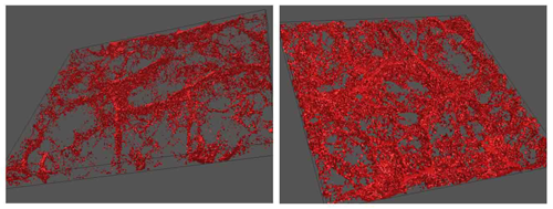
Figure 2: Examples of alpha shapes of the LCDM GIF simulation. Shown are central slices through two alpha shapes (top: low alpha; bottom: high alpha). The image shows the sensitivity of alpha shapes to the topology of the matter distribution. From: Vegter et al. 2010.

II-B Alpha Shape and Topology: Betti numbers

Following the description above, one may find that alpha shapes are intimately related to the topology of a point set. As a result they form a direct and unique way of characterizing the topology of a point distribution. A complete quantitative description of the topology is that in terms of Betti numbers $\beta_{\rm k}$ and these may indeed be directly inferred from the alpha shape.

The Betti number $\beta_{\rm p}$ can be considered as the number of p-dimensional holes of an object or space. Formally, they are the rank of the homology groups $H_{p}$. There is one homology group $H_{p}$ per dimension $p$, and its rank is the p-th Betti number $\beta_{\rm p}$. The first Betti number $\beta_{0}$ specifies the number of independent components of an object. In second Betti number, $\beta_{1}$, may be interpreted as the number of independent tunnels, and $\beta_{2}$ as the number of independent enclosed voids. Tunnels are formed when at a certain $\alpha$ value an edge is added between two vertices that were already connected. When new faces are added, a tunnel can be filled and destroyed and thus leads to the decrease of $\beta_{1}$. Holes are completely surrounded by a surface or faces and disappears when cells are added to the alpha shape.

The Betti numbers completely specify the topology of a manifold in terms of its connectivity. In this sense, they extend the principal topological characterization known in a cosmological context. Numerous cosmological studies have considered the genus of the isodensity surfaces defined by the Megaparsec galaxy distribution [15, 16]. The genus $g$ specifies the number of handles defining a surface and has a direct and simple relation to the Euler characteristic $\chi$ of the manifold, one of the Minkowski functionals. For a manifold consisting of $c$ components we have

$$g\,=\,c\,-\,{1\over 2}\,\chi\,,$$ (2)

where $\chi$ is the integrated intrinsic curvature of the surface,

$$\chi\,=\,{\displaystyle 1\over\displaystyle 2\pi}\,\oint\,\left({\displaystyle 1\over\displaystyle R_{1}R_{2}}\right)\,dS\,.$$ (3)

Indeed, it is straightforward to see that the topological information contained in the Euler characteristic is also represented by the Betti numbers, via an alternating sum relationship. For three-dimensional space, this is

$$\chi\,=\,2\,(\beta_{0}-\beta_{1}+\beta_{2})$$ (4)

While the Euler characteristic and the Betti numbers give information about the connectivity of a manifold, the other three Minkowski functionals are sensitive to local manifold deformations. The Minkowski functionals therefore give information about the geometric and topological properties of a manifold, while the Betti numbers focus only on its topological properties. However, while the Euler characteristic only “summarizes” the topology, the Betti numbers represent a full and detailed characterization of the topology: homeomorphic surfaces will have the same Euler characteristic but two surfaces with the same $\chi$ may not in general be homeomorphic !!!

II-C Computing Betti numbers

For simplicial complexes like Delaunay tessellations and Alpha Shapes, the Betti numbers can be defined on the basis of the oriented $k$-simplices. For such simplicial complexes, the Betti numbers can be computed by counting the number of $k$-cycles it contains. For a three-dimensional alpha shape, a three-dimensional simplicial complex, we can calculate the Betti numbers by cycling over all its constituent simplices. To this end, we base the calculation on the following considerations. When a vertex is added to the alpha complex, a new component is created and $\beta_{0}$ increases by 1. Similarly, if an edge is added, $\beta_{1}$ is increased by 1 if it creates a new cycle, which would be an increase in the number of tunnels. Otherwise, two components get connected so that the number of components is decreased by one: $\beta_{0}$ is decreased by 1. If a face is added, the number of holes is increased by one if it creates a new cycle. Otherwise, a tunnel is filled, so that $\beta_{1}$ is decreased by one. Finally, when a (tetrahedral) cell is added, a hole is filled up and $\beta_{2}$ is lowered by 1.

Following this procedure, the algorithm has to include a technique for determining whether a $k$-simplex belongs to a $k$-cycle. For vertices and cells, and thus 0-cycles and 3-cycles, this is rather trivial. For the detection of 1-cycles and 2-cycles we used a somewhat more elaborate procedure involving union-finding structures [33].

II-D Computational Considerations

For the calculation of the alpha shapes of the point set we resort to the Computational Geometry Algorithms Library, CGAL . Within this context, Caroli & Teillaud recently developed an efficient code for the calculation of two-dimensional and three-dimensional alpha shapes in periodic spaces.

The routines to compute the Betti numbers from the alpha shapes were developed within our own project.

III Alpha Shapes of the Cosmic Web

In a recent study, Vegter et al. computed the alpha shapes for a set of GIF simulations of cosmic structure formation [34, 35]. It concerns a $256^{3}$ particles GIF $N$-body simulation, encompassing a $\Lambda$CDM ($\Omega_{m}=0.3,\Omega_{\Lambda}=0.7,H_{0}=70\,{\rm km/s/Mpc}$) density field within a (periodic) cubic box with length $141h^{-1}{\rm Mpc}$ and produced by means of an adaptive ${\rm P^{3}M}$ $N$-body code [36].

Fig. 2 illustrates the alpha shapes for two different values of $\alpha$, for two-dimensional section through the GIF simulation. The top panel concerns a low value of $\alpha$, the bottom one a high value. The intricacy of the weblike patterns is very nicely followed. The low alpha configuration highlights the interior of filamentary and sheetlike features, and reveals the interconnection between these major structural elements. The high value alpha shape not only covers an evidently larger volume, but does so by connecting to a lot of finer features in the Cosmic Web. Noteworthy are the tenuous filamentary and planar extensions into the interior of the voids.

These images testify of the potential power of alpha shapes in analyzing the weblike cosmic matter distribution, in identifying its morphological elements, their connections and in particular also its hierarchical character.

However, to understand and properly interpret the topological information contained in these images we need first to assess their behaviour in simpler yet similar circumstances. To this end, we introduce a set of heuristic spatial matter distributions, Voronoi clustering models.

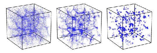
Figure 3: Three different patterns of Voronoi element galaxy distributions, shown in a 3-D cubic setting. The depicted spatial distributions correspond to a wall-dominated Voronoi Universe (left), a filamentary Voronoi Universe (centre) and a cluster-dominated Voronoi Universe (right).

IV Voronoi Clustering Models

Voronoi Clustering Models are a class of heuristic models for cellular distributions of matter which use the Voronoi tessellation as the skeleton of the cosmic matter distribution [37, 38, 39].

The aspect which is modelled in great detail by Voronoi tessellations is that of the large scale clustering of the morphological elements of the Cosmic Web. It is the stochastic yet non-Poissonian geometrical distribution of the walls, filaments and clusters which generates the large-scale clustering properties of matter and the related galaxy populations.

The small-scale distribution of galaxies, i.e. the distribution within the various components of the cosmic skeleton, involves the complicated details of highly nonlinear small-scale interactions of the gravitating matter. Well-defined and elaborate physical models and/or N-body computer simulations might fill in this aspect, although it would lead away from the Voronoi model’s true purpose and conceptual simplicity. In the Voronoi models described here we complement the geometrically fixed configuration of the Voronoi tessellations with a heuristic prescription for the location of particles or model galaxies within the tessellation.

IV-A Voronoi components

According to the Voronoi clustering models, each of the geometric elements of the 3-D Voronoi tessellations is identified with a morphological component of the Cosmic Web. In table I we have listed the various identifications.

Geometric Component	Cosmic Structure
Voronoi Cell	Voids, Field
Voronoi Wall	Walls, Sheets, Superclusters
Voronoi Edge	Filaments, Superclusters
Voronoi Vertex	Clusters

TABLE I: Identification of geometric components in Voronoi tessellations with morphological components of the Cosmic Web.

IV-B Voronoi Element and Voronoi Evolution Models

We distinguish two different yet complementary approaches, “Voronoi Element models” and “Voronoi Evolution models”. Both the Voronoi Element Models and the Voronoi Evolution Models are obtained by projecting an initially random distribution of $N$ sample points/galaxies onto the walls, edges or vertices of the Voronoi tessellation defined by $M$ nuclei. The Voronoi Element Models do this by a heuristic and user-specified mixture of projections on the various geometric elements of the Voronoi skeleton. The Voronoi Evolution Models accomplish this via a gradual motion of the galaxies from their initial random location in their Voronoi cell, directed radially away from the cell’s nucleus.

IV-C Voronoi Element Models

“Voronoi Element models” are fully heuristic models. They are user-specified spatial galaxy distribution within the cells (field), walls, edges and vertices of a Voronoi tessellation. The initially randomly distributed $N$ model galaxies are projected onto the relevant Voronoi wall, Voronoi edge or Voronoi vertex or retained within the interior of the Voronoi cell in which they are located. The field galaxies define a sample of randomly distributed points throughout the entire model volume. The Voronoi Element Models are particularly apt for studying systematic properties of spatial galaxy distributions confined to one or more structural elements of nontrivial geometric spatial patterns.

Simple Voronoi Element Models place their model galaxies exclusively in either walls, edges or vertices. The versatility of the Voronoi element model also allows combinations in which field (cell), wall, filament and vertex distributions are superimposed. These complete composite particle distributions, Mixed Voronoi Element Models, include particles located in four distinct structural components:

1. Field:
             Particles located in the interior of Voronoi cells
            (i.e. randomly distributed across the entire model box)

2. Wall:
              Particles within and around the Voronoi walls.

3. Filament:
       Particles within and around the Voronoi edges.

4. Blobs:
            Particles within and around the Voronoi vertices.

The characteristics of the patterns and spatial distribution in the composite Voronoi Element models can be varied and tuned according to the fractions of galaxies in in Voronoi walls, in Voronoi edges, in Voronoi vertices and in the field. These fractions are free parameters to be specified by the user.

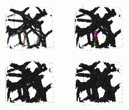
Figure 4: Four alpha shapes of a Voronoi filament model realization. It concerns a sample of 200000 particles in a periodic box of $50~{}h^{-1}{\rm Mpc}$ size with 8 Voronoi cells. From top left to bottom right: $\alpha$=$0.5\times 10^{-4}$, $1.0\times 10^{-4}$, $2\times 10^{-4}$ and $4.0\times 10^{-4}$. See text.

In fig. 3 we have shown three different three-dimensional Simple Voronoi Element Model galaxy distributions. The lefthand model realization corresponds to the model in which galaxies are exclusively located inside walls, a second one where these are concentrated in and around filaments and the third one restricted to galaxies located within clusters.

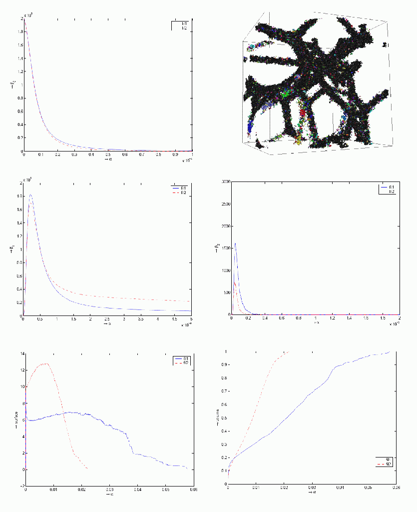
Figure 5: Topological and Geometric parameters Voronoi filament model. For a Voronoi filament model we show an example of an alpha shape (top right), along with the behaviour of five topological parameters as a function of $\alpha$. The different colours of the alpha shape represent the different connected components. Top left: $\beta_{0}$, the number of components of the alpha shape. Centre left: $\beta_{1}$, the number of tunnels in the alpha shape. Centre right: $\beta_{2}$, the number of (surrounded) holes in the alpha shape. Bottom left: total surface area of the alpha shapes. Bottom right: total volume of the alpha shapes. Blue lines: realization with 8 Voronoi cells in box. Red lines: realization with 64 cells in box.

IV-D Voronoi Evolution Models

The second class of Voronoi models is that of the Voronoi Evolution models. They attempt to provide weblike galaxy distributions that reflect the outcome of realistic cosmic structure formation scenarios. They are based upon the notion that voids play a key organizational role in the development of structure and makes the Universe resemble a soapsud of expanding bubbles [40]. While the galaxies move away from the void centres, and stream out of the voids towards the sheets, filaments and clusters in the Voronoi network the fraction of galaxies in the voids (cell interior), the sheets (cell walls), filaments (wall edges) and clusters (vertices) is continuously changing and evolving. The details of the model realization depends on the time evolution specified by the particular Voronoi Evolution Model.

Within the class of Voronoi Evolution Models the most representative and most frequently used are the Voronoi kinematic models. They form the idealized and asymptotic description of the outcome of hierarchical gravitational structure formation process, with single-sized voids forming around depressions in the primordial density field. The Voronoi Kinematic Model “simulates” the asymptotic weblike galaxy distribution implied by the hierarchical void formation process by assuming a single-size dominated void population. It is based upon the notion that voids play a key organizational role in the development of structure and makes the Universe resemble a soapsud of expanding bubbles [40], forming voids forming around a dip in the primordial density field.

This is translated into a scheme for the displacement of initially randomly distributed galaxies within the Voronoi skeleton. Within a void, the mean distance between galaxies increases uniformly in the course of time. When a galaxy tries to enter an adjacent cell, the velocity component perpendicular to the cell wall disappears. Thereafter, the galaxy continues to move within the wall, until it tries to enter the next cell; it then loses its velocity component towards that cell, so that the galaxy continues along a filament. Finally, it comes to rest in a node, as soon as it tries to enter a fourth neighbouring void.

Kinematic Model Configurations
The resulting evolutionary progression within the Voronoi kinematic scheme proceeds from an almost featureless random distribution towards a distribution in which matter ultimately aggregates into conspicuous compact cluster-like clumps.

The steadily increasing contrast of the various structural features is accompanied by a gradual shift in topological nature of the distribution. The virtually uniform and featureless particle distribution at the beginning ultimately unfolds into a highly clumped distribution of almost only clusters (vertices). This evolution involves a gradual progression via a wall-like through a filamentary towards an ultimate cluster-dominated matter distribution. By then nearly all matter has streamed into the nodal sites of the cellular network.

V Topological Analysis of Voronoi Clustering Models

Our topological analysis consists of a study of the systematic behaviour of the Betti numbers $\beta_{0}$, $\beta_{1}$ and $\beta_{2}$, and the surface and volume of the alpha shapes of Voronoi clustering models (see [34, 35]). For each point sample we investigate the alpha shape for the full range of $\alpha$ parameters.

We generated 12 Voronoi clustering models. Each of these contained 200000 particles within a periodic box of size $100~{}h^{-1}{\rm Mpc}$. Of each configuration, we made two realizations, one with 8 centres and Voronoi cells and one with 64. One class of models consisted of pure Voronoi element models. One of these is a pure Voronoi wall model, in which all particles are located within the walls of the Voronoi tessellation. The other is a pure filament model. In addition, there are 4 Voronoi kinematic models, ranging from a mildly evolved to a strongly evolved configuration. In all situations, the clusters, filaments and walls have a finite Gaussian width of $R_{f}=1.0~{}h^{-1}{\rm Mpc}$.

An impression of the alpha shape development may be obtained from the four panels in fig. 4. Different colours depict different individual components of the alpha shape. For the smallest value of $\alpha$, $\alpha=0.5\times 10^{-4}$, we see that the Delaunay simplices contained in the alpha shape delineate accurately nearly all the edges/filaments in the particle distribution. As $\alpha$ increase, going from the topleft panel down to the bottom right one, we find that the alpha shape fills in the planes of the Voronoi tessellation. For even larger values of $\alpha$, the alpha shape includes the larger Delaunay simplices that are covering part of the interior of the Voronoi cells. It is a beautiful illustration of the way in which alpha shapes define, as it were, naturally evolving surfaces that are sensitive to every detail of the morphological and topological structure of the cosmic matter distribution.

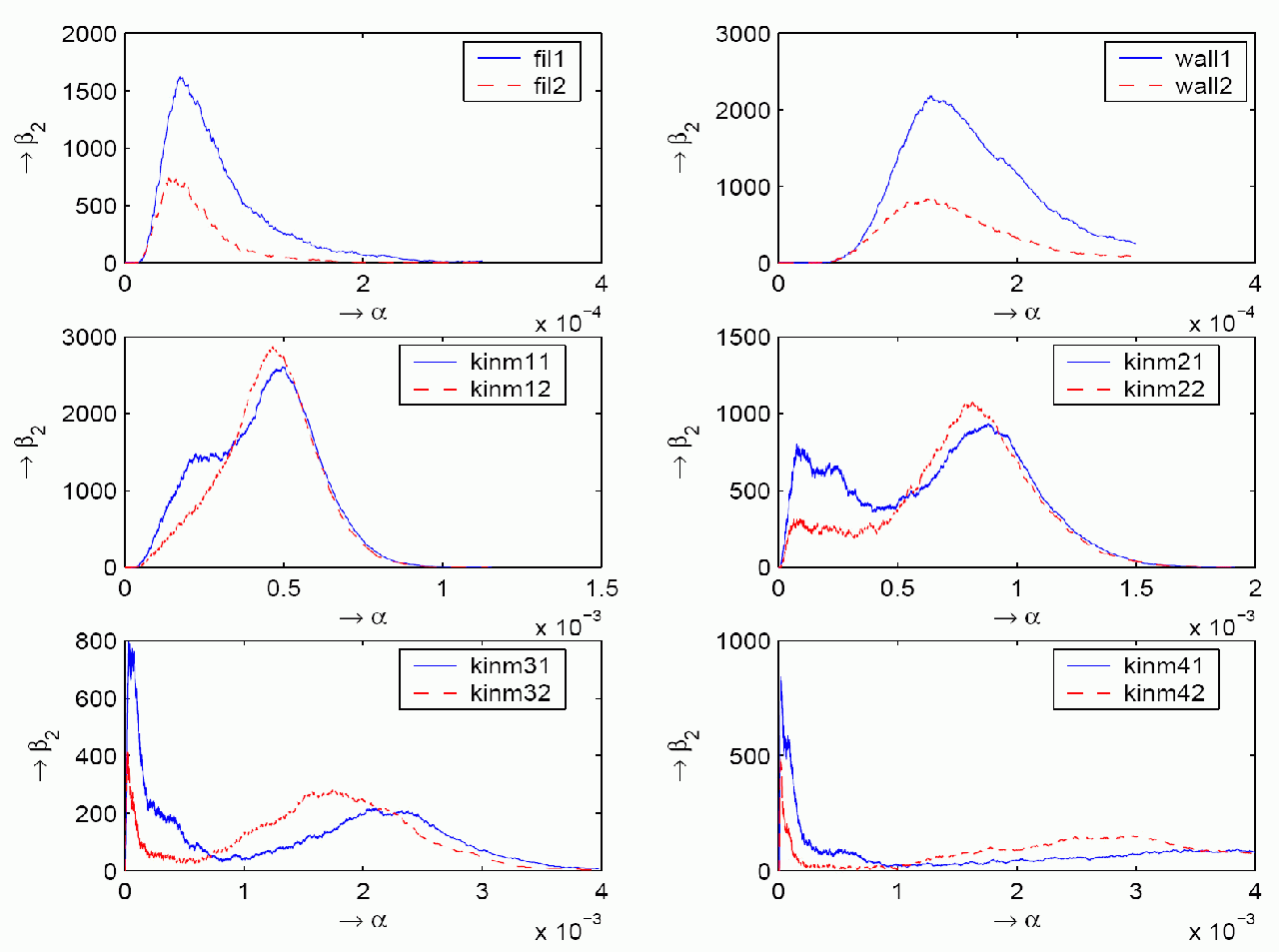
Figure 6: Third Betti number $\beta_{2}$ for different clustering models. Shown are the curves $\beta_{2}(\alpha)$ for six Voronoi clustering models. Top left: Voronoi filament model. Top right: Voronoi wall model. Centre left to Bottom right panel: four stages of the Voronoi kinematic model, going from a moderately evolved model dominated by walls (centre left) to a highly evolved one dominated by filaments and clusters (bottom right).

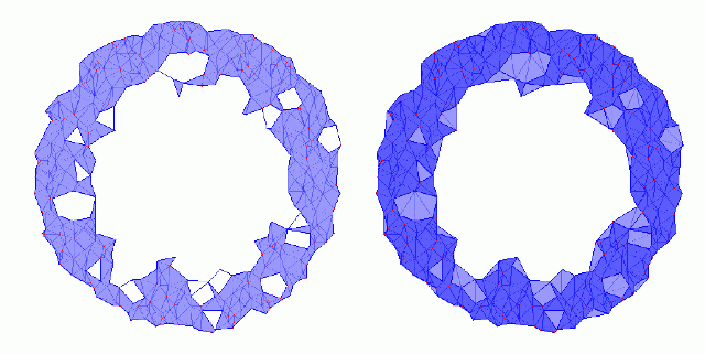
Figure 7: Cartoon illustrating the idea of persistence. Two alpha shapes corresponding to a random point distribution on the surface of a torus. The alpha shape on the left has 18 holes, of which only the central one is significant. The alpha shape on the right, corresponding to a larger $\alpha$ contains this one hole.

V-A Filament Model topology

We take the Voronoi filament model as a case study. Its topology and geometry is studied by following the behaviour of the three Betti numbers $\beta_{0}$, $\beta_{1}$ and $\beta_{2}$ of the corresponding alpha shapes as a function of the parameter $\alpha$. Also we adress two of the Minkowski functionals for the alpha shapes, namely their volume and surface area (note that the Euler characteristic is already implicitly included in the Betti numbers).

Fig. 5 shows the relation between the Betti numbers, surface and volume of the alpha shapes and the value of $\alpha$. The first Betti number, $\beta_{0}$, decreases monotonously as $\alpha$ increases. This Betti number specifies the number of isolated components in the alpha shape, and at $\alpha=0$ it is equal to the number of points of the sample, $\beta_{0}(\alpha=0)=200000$. At larger $\alpha$, more and more components merge into larger entities, which explains the gradual decrease of $\beta_{0}$ with increasing $\alpha$.

The second Betti number, $\beta_{1}$, represent the number of independent tunnels. At first, at small values of $\alpha$ it increases steeply, as the large number of individual components grow as more Delaunay edges are added to them. Once isolated components start to fill up and merge with others, at values $\alpha>0.25\times 10^{-4}$, we see a steep decrease of the Betti number $\beta_{1}$.

In the case of the singly morphological distribution of the Voronoi filament model the third Betti number, $\beta_{2}$, has a behaviour resembling that of $\beta_{1}$: a peaked distribution around a finite value of $\alpha$. This Betti number represents the number of holes in the alpha shape and it is easy to understand that at small $\alpha$ values this number quickly increases as each of the individual alpha shape components gets extended with new Delaunay simplices. However, once $\alpha$ gets beyond a certain value this will include more and more tetrahedra. These start to fill up the holes. Notice that in the given example of the Voronoi filament model this occurs at $\alpha\approx 0.45\times 10^{-4}$ (also see fig. 6), substantially beyond the peak in the $\beta_{1}$ distribution: on average larger values of $\alpha$ are needed to add complete Delaunay tetrahedra to the alpha shape.

We also studied two additonal Minkowski functionals, volume and surface, to assess the geometrical properties of the evolving alpha shapes of the Voronoi filament models. The results are shown in the bottom panels of fig. 5. Evidently, the volume of the alpha shape increases monotonously as $\alpha$ becomes larger and more and more tetrahedral cells become part of the alpha shape. The surface area has a somewhat less straightforward behaviour. Over a substantial range the surface area grows mildy as individual components of the alpha shape grow. When these components start to merge, and especially when holes within the components get filled up, the surface area shrinks rapidly. Once, the whole unit cube is filled, the surface area has shrunk to zero.

V-B Betti Systematics

Having assessed one particular Voronoi clustering model in detail, we may try to identify the differences between the different models. While this is still the subject of ongoing research, we find substantial differences between the models on a few particular aspects. Here we discuss two in more detail:

Number of components: $\beta_{0}$
While for all models the curve $\beta_{0}(\alpha)$ is a monotonously decreasing function of $\alpha$, the range over which $\beta_{0}$ differs substantially from unity and the rate of decrease are highly sensitive to the underlying distribution. In fact, the derivative $\partial\beta_{0}/\partial\alpha$ contains interesting features, like a minimum and a varying width, which are potentially interesting for discriminating between the underlying topologies.

Number of holes: $\beta_{2}$
The most outstanding Betti number is $\beta_{2}$, i.e. the number of holes in an alpha shape. As one may infer from fig. 6, substantial and systematic differences between different models can be observed. This concerns not only the values and range over which $\beta_{2}$ reaches a maximum, as for the pure filament and wall models, but even entirely different systematic behaviour in the case of the more elaborate and complex Voronoi kinematic models (see e.g. the review by Van de Weygaert 2010 [41] and [39]).

In the case of the kinematic models we find more than one peak in the $\beta_{2}(\alpha)$ distribution, each corresponding to different morphological components of the particle distribution. In this respect, it is revealing to see follow the changes in $\beta_{2}(\alpha)$ as we look at different evolutionary stages.

The four panels from centre left to bottom right in fig. 6 correspond to four different stages of evolution. The centre left one concerns a moderately evolved matter distribution, dominated by walls. The centre right panel corresponds to a stage at which walls and filaments are approximately equally prominent. The bottom left panel is a kinematic model in which filaments represent more than $40\%$ of the mass, while walls and the gradually more prominent clusters each represent around $25\%$ of the particles. The final bottom right diagram corresponds to a highly evolved mass distribution, with clusters and filaments representing each around $40\%$ of the particles.

The different morphological patterns of the Voronoi kinematic models are strongly reflected in the behaviour of $\beta_{2}(\alpha)$. In the centre left panel we find a strong peak at $\alpha\approx 5\times 10^{-4}$, with a shoulder at lower values. The peak reflects the holes defined by the walls in the distribution, while the shoulder finds its origin in the somewhat smaller holes defined by filaments: the average distance between walls is in the order of the Voronoi cell size, while the average filament distance is more related to the Voronoi wall size. The identity of the peaks becomes more clear when turning to the two peak distribution in the centre right panel, in which the strong peak at $\alpha\approx 1\times 10^{-4}$ is a direct manifestation of the strongly emerged filaments in the matter distribution. As the shift to filaments and clusters continues, we even see the rise of a third peak at much smaller values of $\alpha$ (bottom panels). This clearly corresponds to the holes in the high density and compact cluster regions.

VI Conclusions and Prospects: Persistence

We have established the promise of alpha shapes for measuring the topology of Megaparsec galaxy distribution in the Cosmic Web by studying the Betti numbers and several Minkowski functionals of a set of heuristic Voronoi clustering models. Alpha Shape analysis has the great advantage of being self-consistent and natural, involving shapes and surfaces that are entirely determined by the point distribution, independent of any artificial filtering.

The one outstanding issue we have not adressed is that of noise in the dataset. Discrete point distributions are necessarily beset by shotnoise. As a result, the alpha shapes will reflect the noise in the point distribution. The induced irregularities in the alpha shapes induce holes and tunnels which do not represent any real topological structure but nonetheless influence the values of the Betti numbers.

Edelsbrunner et al. (2000) [42] introduced the concept of persistence to seek to filter out the insignificant structures (see also [23], and [25] for a detailed and insightful review). The basic idea is that holes and tunnels that remain in existence over a range of $\alpha$ values are significant and should be included in the Betti number calculation. The range is a user-defined persistence parameter $p$. The implementation of the concept of persistence in our topological study will be adressed in forthcoming work.

References

- [1] J. Bond, L. Kofman, and D. Pogosyan, “How filaments are woven into the cosmic web,” Nature, vol. 380, pp. 603–606, 1996.
- [2] R. van de Weygaert and J. R. Bond, “Observations and Morphology of the Cosmic Web,” in A Pan-Chromatic View of Clusters of Galaxies and the Large-Scale Structure, ser. Lecture Notes in Physics, Berlin Springer Verlag, M. Plionis, O. López-Cruz, & D. Hughes, Ed., vol. 740, 2008, pp. 409–+.
- [3] M. Colless and 2dF consortium, “The 2df galaxy redshift survey: Final data release,” pp. 1–32, 2003, astroph/0306581.
- [4] M. Tegmark and et al., “The three-dimensional power spectrum of galaxies from the sloan digital sky survey,” Astrophys. J., vol. 606, pp. 702–740, 2004.
- [5] J. Huchra and et al., “The 2mass redshift survey and low galactic latitude large-scale structure,” in Nearby Large-Scale Structures and the Zone of Avoidance, ser. ASP Conf. Ser. Vol., A. Fairall and P. Woudt, Eds., vol. 239. Astron. Soc. Pacific, San Francisco, 2005, pp. 135–146.
- [6] P. Peebles, The Large Scale Structure of the Universe. Princeton Univ. Press, 1980.
- [7] R. van de Weygaert and J. R. Bond, “Clusters and the Theory of the Cosmic Web,” in A Pan-Chromatic View of Clusters of Galaxies and the Large-Scale Structure, ser. Lecture Notes in Physics, Berlin Springer Verlag, M. Plionis, O. López-Cruz, & D. Hughes, Ed., vol. 740, 2008, pp. 335–+.
- [8] V. Springel and et al., “Simulations of the formation, evolution and clustering of galaxies and quasars,” Nature, vol. 435, pp. 629–636, 2005.
- [9] H. Edelsbrunner, D. Kirkpatrick, and R. Seidel, “On the shape of a set of points in the plane,” IEEE Trans. Inform. Theory, vol. 29, pp. 551–559, 1983.
- [10] A. Babul and G. D. Starkman, “A quantitative measure of structure in the three-dimensional galaxy distribution - Sheets and filaments,” Astrophys. J., vol. 401, pp. 28–39, Dec. 1992.
- [11] S. Luo and E. Vishniac, “Three-dimensional shape statistics: Methodology,” Astrophys. J. Suppl., vol. 96, pp. 429–460, Feb. 1995.
- [12] S. Basilakos, M. Plionis, and M. Rowan-Robinson, “PSCz superclusters: detection, shapes and cosmological implications,” Mon. Not. R. Astron. Soc., vol. 323, pp. 47–55, May 2001.
- [13] K. Mecke, T. Buchert, and H. Wagner, “Robust morphological measures for large-scale structure in the universe,” Astron. Astrophys., vol. 288, pp. 697–704, 1994.
- [14] J. Schmalzing, T. Buchert, A. Melott, V. Sahni, B. Sathyaprakash, and S. Shandarin, “Disentangling the cosmic web. i. morphology of isodensity contours,” Astrophys. J., vol. 526, pp. 568–578, 1999.
- [15] J. Gott, M. Dickinson, and A. Melott, “The sponge-like topology of large-scale structure in the universe,” Astrophys. J., vol. 306, pp. 341–357, 1986.
- [16] F. Hoyle, M. S. Vogeley, J. R. Gott, III, M. Blanton, M. Tegmark, D. H. Weinberg, N. Bahcall, J. Brinkmann, and D. York, “Two-dimensional Topology of the Sloan Digital Sky Survey,” Astrophys. J., vol. 580, pp. 663–671, Dec. 2002.
- [17] V. Sahni, B. Sathyprakash, and S. Shandarin, “Shapefinders: A new shape diagnostic for large-scale structure,” Astrophys. J., vol. 507, pp. L109–L112, 1998.
- [18] S. F. Shandarin, J. V. Sheth, and V. Sahni, “Morphology of the supercluster-void network in CDM cosmology,” Mon. Not. R. Astron. Soc., vol. 353, pp. 162–178, Sep. 2004.
- [19] V. Martínez, J.-L. Starck, E. Saar, D. Donoho, S. R. S.C., P. de la Cruz, and S. Paredes, “Morphology of the galaxy distribution from wavelet denoising,” Astrophys. J., vol. 634, pp. 744–755, 2005.
- [20] E. Saar, V. J. Martínez, J. Starck, and D. L. Donoho, “Multiscale morphology of the galaxy distribution,” Mon. Not. R. Astron. Soc., vol. 374, pp. 1030–1044, Jan. 2007.
- [21] E. Muecke, Shapes and Implementations in three-dimensional geometry, 1993, phD thesis, Univ. Illinois Urbana-Champaign.
- [22] H. Edelsbrunner and E. Muecke, “Three-dimensional alpha shapes,” ACM Trans. Graphics, vol. 13, pp. 43–72, 1994.
- [23] H. Edelsbrunner, D. Letscher, and A. Zomorodian, “Topological persistance and simplification,” Discrete and Computational Geometry, vol. 28, pp. 511–533, 2002.
- [24] H. Edelsbrunner, “Alpha shapes - a survey,” in Tessellations in the Sciences; Virtues, Techniques and Applications of Geometric Tilings, J. R. . V. I. R. van de Weygaert, G. Vegter, Ed. Springer Verlag, 2010.
- [25] H. Edelsbrunner and J. Harer, Computational Topology, An Introduction. American Mathematical Society, 2010.
- [26] T. Dey, H. Edelsbrunner, and S. Guha, “Computational topology,” in Advances in Discrete and Computational Geometry, B. Chazelle, J. Goodman, and R. Pollack, Eds. American Mathematical Society, 1999, pp. 109–143.
- [27] G. Vegter, “Computational topology,” in Handbook of Discrete and Computational Geometry, 2nd edition, J. E. Goodman and J. O’Rourke, Eds. Boca Raton, FL: CRC Press LLC, 2004, ch. 32, pp. 719–742.
- [28] A. Zomorodian, Topology for Computing, ser. Cambr. Mon. Appl. Comp. Math. Cambr. Univ. Press, 2005.
- [29] H. Edelsbrunner, M. Facello, and J. Liang, “On the definition and the construction of pockets in macromolecules,” Discrete Appl. Math., vol. 88, pp. 83–102, 1998.
- [30] J. Liang, H. Edelsbrunner, P. Fu, P. Sudhakar, and S. Subramaniam, “Analytical shape computation of macromolecules: I. molecular area and volume through alpha shape,” Proteins: Structure, Function, and Genetics, vol. 33, pp. 1–17, 1998.
- [31] ——, “Analytical shape computation of macromolecules: Ii. inaccessible cavities in proteins,” Proteins: Structure, Function, and Genetics, vol. 33, pp. 18–29, 1998.
- [32] J. Liang, C. Woodward, and H. Edelsbrunner, “Anatomy of protein pockets and cavities: measurement of binding site geometry and implications for ligand design,” Protein Science, vol. 7, pp. 1884–1897, 1998.
- [33] C. J. A. Delfinado and H. Edelsbrunner, “An incremental algorithm for betti numbers of simplicial complexes,” in Symposium on Computational Geometry, 1993, pp. 232–239.
- [34] B. Eldering, Topology of Galaxy Models, 2006, mSc thesis, Univ. Groningen.
- [35] G. Vegter, R. van de Weygaert, E. Platen, N. Kruithof, and B. Eldering, “Alpha shapes and the topology of cosmic large scale structure,” Mon. Not. R. Astron. Soc., 2010, in prep.
- [36] G. Kauffmann, J. M. Colberg, A. Diaferio, and S. D. M. White, “Clustering of galaxies in a hierarchical universe - I. Methods and results at z=0,” Mon. Not. R. Astron. Soc., vol. 303, pp. 188–206, Feb. 1999.
- [37] R. van de Weygaert and V. Icke, “Fragmenting the universe. II - Voronoi vertices as Abell clusters,” Astron. Astrophys., vol. 213, pp. 1–9, Apr. 1989.
- [38] R. van de Weygaert, Voids and the geometry of large scale structure, 1991, phD thesis, University of Leiden.
- [39] R. v. d. Weygaert, “Voronoi tessellations and the cosmic web: Spatial patterns and clustering across the universe,” in ISVD ’07: Proceedings of the 4th International Symposium on Voronoi Diagrams in Science and Engineering. Washington, DC, USA: IEEE Computer Society, 2007, pp. 230–239.
- [40] V. Icke, “Voids and filaments,” Mon. Not. R. Astron. Soc., vol. 206, pp. 1P–3P, Jan. 1984.
- [41] R. van de Weygaert, “Voronoi clustering models of the cosmic web,” in Tessellations in the Sciences; Virtues, Techniques and Applications of Geometric Tilings, J. R. . V. I. R. van de Weygaert, G. Vegter, Ed. Springer Verlag, 2010.
- [42] H. Edelsbrunner, D. Letscher, and A. Zomorodian, “Topological persistence and simplification,” in FOCS, 2000, pp. 454–463.