Long-range correlations and ensemble inequivalence in a generalized ABC model

Abstract

A generalization of the ABC model, a one-dimensional model of a driven system of three particle species with local dynamics, is introduced, in which the model evolves under either (i) density-conserving or (ii) nonconserving dynamics. For equal average densities of the three species, both dynamical models are demonstrated to exhibit detailed balance with respect to a Hamiltonian with long-range interactions. The model is found to exhibit two distinct phase diagrams, corresponding to the canonical (density-conserving) and grand canonical (density nonconserving) ensembles, as expected in long-range interacting systems. The implication of this result to nonequilibrium steady states, such as those of the ABC model with unequal average densities, are briefly discussed.

In many cases nonequilibrium systems driven by an external field, such as the temperature gradient or electric field, reach a nonequilibrium steady state which is characterized by long-range correlations Spohn1983 . In some cases such long-range correlations lead to phenomena like the emergence of long-range order and spontaneous symmetry breaking, even when the dynamics is local and stochastic Mukamel2000 . This is particularly intriguing in one-dimensional models, where such phenomena do not exist under equilibrium conditions for systems with short-range interactions at finite temperatures.

A model which is often discussed in this context is the ABC model Evans1998 ; Clincy2003 ; Ayyer2009 . This is a one-dimensional three species model of a driven system with local dynamics which exhibits phase separation at nonvanishing densities of the three species. It has been shown that at a particular point of its phase space, namely, for equal densities of the three species, the model obeys detailed balance, and the steady-state distribution can be expressed in terms of an effective Hamiltonian with long-range interactions. Thus, although the dynamics is local and stochastic, the long-range nature of the resulting effective interactions leads to phase separation and long-range order.

Equilibrium systems with short-range interactions typically evolve into a unique state which is independent of their dynamics. Thus, for instance, the Ising models with magnetization-conserving (Kawasaki) dynamics and nonconserving (Glauber) dynamics result in the same equilibrium state. This equivalence of ensembles is broken in systems with long-range interactions, where the two-body potential decays at large distance with a power smaller than the spatial dimension. Such systems are nonadditive and their thermodynamic functions are superextensive with respect to their size. As a result, they exhibit unusual phenomena such as ensemble inequivalence, negative specific heat, and slow relaxation dynamics (see, for example, Thirring1970 ; Mukamel2010 ; Campa2009 ). The ABC model is expected to share some of these properties at the equal densities point, where it behaves as an effective long-range interacting system. A different mechanism for ensemble inequivalence has been discussed within the context of the zero-range process, whereby long-range order emerges in one dimension due to the noncompactness of the local order parameter Grosskinsky2008 .

In this Letter, we generalize the ABC model to include vacancies and nonconserving processes. This allows us to compare the phase diagram of the conserving model with that of the nonconserving model. We show that for equal densities both dynamics obey detailed balance with respect to a Hamiltonian with long-range interactions. Under conserving dynamics, where the nonconserving processes are excluded, the resulting steady state is that of the canonical ensemble. The nonconserving dynamics correspond to the grand canonical ensemble. Evaluating the phase diagram of the generalized model, we find that, as is common in systems with long-range interactions, the canonical and the grand canonical ensembles are inequivalent, yielding different phase diagrams.

Small deviations from the equal densities condition are not expected to significantly alter the steady state. Thus, a detailed study of the model with equal densities may serve as a guideline for investigation of the general case with nonequal densities, where detailed balance is not satisfied and an effective energy cannot be defined. This may shed some light on the mechanisms leading to long-range phenomena in nonequilibrium steady states.

We begin by outlining the main features of the ABC model on a ring Evans1998 . The model consists of three species of particles, labeled $A,\,B$, and $C$, which occupy the sites of a periodic lattice of length $L$. The number of particles of each type is given by $N_{A},\,N_{B}$, and $N_{C}$ with $N_{A}+N_{B}+N_{C}=L$. The model evolves by local, random sequential dynamics whereby two neighboring particles are exchanged clockwise with the following rates:

$$AB\overset{q}{\underset{1}{\rightleftarrows}}BA\,;\,BC\overset{q}{\underset{1}{\rightleftarrows}}CB\,;\,CA\overset{q}{\underset{1}{\rightleftarrows}}AC.$$ (1)

For $q=1$ the dynamics is symmetric and the system relaxes to a homogeneous state, in which all particles are uniformly distributed, regardless of type. For $q\neq 1$ the system reaches a nonequilibrium steady state in which the particles phase separate into three domains. The domains are arranged, clockwise, in the order $AA\ldots ABB\ldots BCC\ldots C$ for $q<1$ and counterclockwise for $q>1$. We will assume $q<1$ for the rest of the Letter. It has been shown that at equal densities, $N_{A}=N_{B}=N_{C}=L/3$, the dynamics obeys detailed balance with respect to the Hamiltonian

$$\mathcal{H}\left(\left\{X_{i}\right\}\right)=\sum_{i=1}^{L-1}\sum_{j=1}^{L-i}\left(A_{i}C_{i+j}+B_{i}A_{i+j}+C_{i}B_{i+j}\right).$$ (2)

Here $\left\{X_{i}\right\}=\left\{A_{i},B_{i},C_{i}\right\}$,

$$A_{i}=\left\{\begin{array}[]{cc}1&{\rm if\,site\,}i{\rm\,is\,occupied\,by\,an\,}A{\rm\,particle}\\ 0&{\rm otherwise,}\end{array}\right.$$ (3)

and similarly for $B_{i}$ and $C_{i}$. The change in $\mathcal{H}$ due to the exchange of any pair of neighboring particles as described in (1) is $\Delta\mathcal{H}=\pm 1$, where, for example, the exchange of $AB$ to $BA$ raises the energy by $1$. Detailed balance is thus maintained with respect to the steady-state distribution $P\left(\left\{X_{i}\right\}\right)=q^{\mathcal{H}\left(\left\{X_{i}\right\}\right)}/Z_{L}$, with the partition sum $Z_{L}=\sum_{\left\{X_{i}\right\}}q^{\mathcal{H}\left(\left\{X_{i}\right\}\right)}$. While the microscopic dynamics (1) is strictly local, the interactions in $\mathcal{H}$ are long-ranged (mean-field like).

It has been demonstrated that, by considering an L-dependent $q$ which approaches $1$ sufficiently fast at large L, the $q=1$ homogeneous state may be realized Clincy2003 . For $q=\exp\left(-\beta/L\right)$, the model exhibits a phase transition from a homogeneous state for $\beta<\beta_{c}$ to a phase-separated state for $\beta>\beta_{c}$, with $\beta_{c}=2\pi\sqrt{3}$ . The parameter $\beta$ serves as an inverse temperature.

We now generalize the model, allowing us to compare conserving and nonconserving dynamics. As a first step we introduce vacancies into the model. Thus, each site may be occupied either by one of the three species or by a vacancy $0$. Hence, $N\equiv N_{A}+N_{B}+N_{C}\leq L$. The dynamics is such that vacancies are neutral, so that a particle of any species may hop to the left or right into an empty site with equal probability. The following rule is added to the exchange rules Eq. (1):

$$X0\overset{1}{\underset{1}{\rightleftarrows}}0X\,,\;X=A,B,C.$$ (4)

Next, we add nonconserving processes, whereby particles are allowed to leave and enter the system in ordered groups of three neighboring particles:

$$ABC\overset{pq^{3\mu L}}{\underset{p}{\rightleftarrows}}000,$$ (5)

where $\mu$ is a chemical potential, taken to be equal for all three species, and $p$ is a parameter whose value does not affect the steady state in the case where detailed balance is satisfied. This particular choice of the nonconserving process maintains equal densities whenever the initial configuration satisfies this condition.

Focusing on the case of equal densities, we consider two alternative dynamics: (i) density-conserving dynamics where the evolution takes place by the processes (1) and (4) and (ii) nonconserving dynamics where all processes (1), (4) and (5) are allowed. Under both dynamics, detailed balance is satisfied with respect to the following Hamiltonian:

$$\tilde{\mathcal{H}}\left(\left\{X_{i}\right\}\right)=\mathcal{H}\left(\left\{X_{i}\right\}\right)-\frac{N\left(N-1\right)}{6}-\mu NL.$$ (6)

In the conserving case, the chemical potential term is constant and may be omitted. Note that, while the generalized ABC dynamics is strictly local, the Hamiltonian is long-ranged. The fact that detailed balance is satisfied with respect to the particle-conserving processes (1) and (4) is a result of the neutrality of the vacancies. The reason why detailed balance is also satisfied with respect to the nonconserving processes (5) has to do with the fact that the energy $E$ of a configuration is invariant under any translation of $ABC$ triplets, namely, $E(\ldots YABC\ldots)=E(\ldots ABCY\ldots)$, where $Y$ stands for either a particle of any species or a vacancy. Thus, the rates of depositing or evaporating $ABC$ triplets could be taken as independent of the microscopic configuration in which these processes take place, as given by the rates (5). The change in energy corresponding to depositing an $ABC$ triplet in a system containing $N$ particles is given by $\Delta\tilde{\mathcal{H}}=N+1-\frac{1}{6}\left(6N+6\right)-3\mu L=-3\mu L$. Thus, detailed balance is satisfied with respect to (5).

The conserving dynamics leads to the canonical steady state of the Hamiltonian (6), while the nonconserving dynamics leads to the grand canonical one. As a result of the long-range nature of the interactions, the two ensembles need not be equivalent, yielding different phase diagrams. In order to carry out this analysis we take $q=\exp\left(-\beta/L\right)$ and turn to the continuum limit Clincy2003 ; Ayyer2009 . The local concentration of $A,\,B$, and $C$ particles at the point $x=i/L$ is represented by the density profile $\rho_{n}(x)\;(n=A,B,C)$ with $\rho(x)=\rho_{A}(x)+\rho_{B}(x)+\rho_{C}(x)$. The steady-state distribution of the density profiles is given by $P\left[\rho_{n}(x)\right]=\exp\left\{-L\mathcal{F}\left[\rho_{n}(x)\right]\right\}$, where $\mathcal{F}\left[\rho_{n}(x)\right]$ is the free energy functional. The equilibrium profile can thus be found by minimizing the free energy functional with respect to $\rho_{n}(x)$ under the equal densities condition $\int_{0}^{1}\rho_{n}(x)dx\equiv r/3$.

We begin by considering the conserving dynamics (i), where the overall density $r$ is fixed, and the free energy functional is

$$\mathcal{F}[\rho_{n}(x)]=\int_{0}^{1}dx[\rho_{A}(x)\ln\rho_{A}(x)+\rho_{B}(x)\ln\rho_{B}(x)$$

$$+\rho_{C}(x)\ln\rho_{C}(x)+(1-\rho(x))\ln(1-\rho(x))]$$

$$+\beta\left(\int_{0}^{1}dx\int_{0}^{1-x}dz[\rho_{A}(x)\rho_{C}(x+z)\right.$$

$$\left.+\rho_{B}(x)\rho_{A}(x+z)+\rho_{C}(x)\rho_{B}(x+z)]-\frac{1}{6}r^{2}\right).$$ (7)

Here the first term corresponds to the entropy, and the second term corresponds to the energy.

At high temperatures $T\equiv 1/\beta$, the free energy is minimized by the homogeneous density profiles $\rho_{n}(x)=r/3$, corresponding to the disordered phase. In order to find the transition, we note that in the ordered phase the density profiles are expected to satisfy $\rho_{B}(x)=\rho_{A}(x-1/3)$ and $\rho_{C}=\rho_{A}(x+1/3)$. Assuming a smooth transition to the ordered phase we expand $\rho_{A}(x)$ close to the homogeneous solution:

$$\rho_{A}(x)=\frac{r}{3}+\sum_{m=1}^{\infty}a_{m}\cos(2\pi mx).$$ (8)

This profile is arbitrarily chosen among all its translationally related degenerate profiles. Substituting (8) in Eq. (7), together with the symmetry conditions on $\rho_{B}(x)$ and $\rho_{C}(x)$, results in a series expansion for the free energy $\mathcal{F}$ in powers of the amplitudes $a_{m}$. Instabilities of the homogeneous state are dominated by the first mode $a_{1}$, while higher modes $a_{m}$ are driven by it. Applying the equilibrium conditions $\partial\mathcal{F}/\partial a_{m}=0$, one can express the coefficients $a_{m}$ for $m>1$ in powers of $a_{1}$. This leads to a Landau expansion for the free energy $\mathcal{F}$, with $a_{1}$ serving as an order parameter:

$$\mathcal{F}[\rho_{A}(x)]=\mathcal{F}\left(\frac{r}{3}\right)+f_{2}a_{1}^{2}+f_{4}a_{1}^{4}+\ldots,$$ (9)

where

$$f_{2}=\frac{9}{4r}-\frac{3\sqrt{3}\beta}{8\pi}\,;\,f_{4}=\frac{81}{32r^{3}}\left(\frac{\sqrt{3}\beta r+6\pi}{\sqrt{3}\beta r+12\pi}\right).$$ (10)

Since $f_{4}>0$ for any $r$ and $\beta$, there is a second-order phase transition at $f_{2}=0$, where $\beta_{c}=2\pi\sqrt{3}/r$.

By evaluating the chemical potential using $\mu=\frac{1}{\beta}\frac{\partial}{\partial r}\mathcal{F}\left(r/3\right)$, the critical line is obtained:

$$\mu=\frac{1}{\beta}\left[\ln\left(\frac{2\pi}{\sqrt{3}\beta}\right)-\ln\left(1-\frac{2\pi\sqrt{3}}{\beta}\right)\right].$$ (11)

The $(1/\beta,\mu)$ phase diagram is shown in Fig. 1.

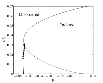
Figure 1: The $(1/\beta,\mu)$ phase diagram of the ABC model. For conserving dynamics the model exhibits a line of continuous transition [thin solid line, Eq. (11)]. For nonconserving dynamics the model exhibits a multicritical (fourth-order) point (star), beyond which the transition becomes first-order (thick solid line) determined numerically (circles).

In order to evaluate the phase diagram corresponding to the nonconserving dynamics (ii), we consider the Gibbs free energy $\mathcal{G}[\rho_{n}(x)]=\mathcal{F}\left[\rho_{n}(x)\right]-\beta\mu r$ and study the stability of the homogeneous phase at a given chemical potential $\mu$. To this end we expand $\mathcal{G}$ in small deviations from the homogeneous profile. Here, however, one should also allow for variations of the overall density $\delta r$. Thus, the $A$-particle density profile close to the transition can be written as

$$\rho_{A}(x)=\frac{r}{3}+\frac{\delta r}{3}+\sum_{m=1}^{\infty}a_{m}\cos(2\pi mx).$$ (12)

As before, the $B$ and $C$ density profiles are obtained by translation operations. The equilibrium conditions $\partial\mathcal{G}/\partial\left(\delta r\right)=0$ and $\partial\mathcal{G}/\partial a_{m}=0$, for $m>1$ result in the Landau expansion of $\mathcal{G}$ in terms of $a_{1}$,

$$\mathcal{G}\left[\rho_{A}(x)\right]=\mathcal{G}\left(\frac{r}{3}\right)+g_{2}a_{1}^{2}+g_{4}a_{1}^{4}+g_{6}a_{1}^{6}+\ldots\leavevmode\nobreak\ ,$$ (13)

$$\mathrm{with\leavevmode\nobreak\ \leavevmode\nobreak\ \leavevmode\nobreak\ \leavevmode\nobreak\ \leavevmode\nobreak\ \leavevmode\nobreak\ \leavevmode\nobreak\ \leavevmode\nobreak\ }g_{2}=f_{2}=\frac{9}{4r}-\frac{3\sqrt{3}\beta}{8\pi}\leavevmode\nobreak\ .$$ (14)

This coefficient vanishes at $\beta_{c}=2\pi\sqrt{3}/r$, yielding the critical line, as long as $g_{4}>0$. On the critical line the fourth-order coefficient is given by

$$g_{4}\left(\beta_{c}\right)=\frac{27}{32r^{3}}\left(3r-1\right)\leavevmode\nobreak\ .$$ (15)

The transition is, thus, continuous for $r>1/3$, becoming first-order at a multicritical point (MCP) $r=1/3$, where $g_{2}=g_{4}=0$. In the $\left(1/\beta,\mu\right)$ plane, the MCP is given by

$$\beta_{{\rm MCP}}=6\pi\sqrt{3}\;;\;\mu_{{\rm MCP}}=-\frac{\ln 6}{6\pi\sqrt{3}}\simeq-0.0549.$$ (16)

Calculating higher-order terms in the expansion (13), we find that at the MCP $g_{6}=0$ while $g_{8}>0$, which implies that this is a fourth-order critical point.

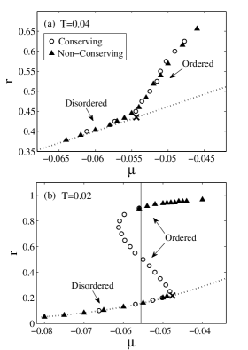
Figure 2: The $r(\mu)$ curve obtained from Monte Carlo simulations with $L=1800$ and temperatures (a) above and (b) below the multicritical point. In (a) the two types of dynamics result in the same curve with a continuous transition. The expected critical point is marked by $\mathbf{x}$; deviations are due to the finite size of the system. In (b) the conserving dynamics results in a continuous transition ($\mathbf{x}$), while the nonconserving dynamics displays a discontinuity in $r$ at a first-order transition. Hysteretic behavior is observed. The expected transition point obtained by minimization of $\mathcal{G}$ is indicated by the vertical line. Dotted lines correspond to homogeneous profiles.

To complete the phase diagram we note that at $T=0$ the system is fully phase-separated, with randomly distributed vacancies. For such states one has $\mathcal{G}_{T=0}=-r^{2}/18-\mu r$. Minimizing $\mathcal{G}$ with respect to $r$, one finds a first-order transition at $\mu=-1/18$ between an empty state $(r=0)$ for $\mu<-1/18$ and a phase-separated state with $r=1$ for $\mu>-1/18$. The first-order line connecting the MCP and the $T=0$ transition point is found numerically by integrating the dynamical equations $\partial\rho_{n}(x,t)/\partial t=-\delta\mathcal{G}/\delta\rho_{n}(x,t)$. While these equations do not represent the actual dynamics of the system, their steady-state solution reproduces the steady-state profile corresponding to the minimum of $\mathcal{G}$.

The phase diagram of the nonconserving ABC model is given in Fig. 1, where it is compared with that of the conserving model. While the transition to the phase-separated state in the conserving model is continuous throughout the $(1/\beta,\mu)$ plane, the transition in the nonconserving model changes character at a fourth-order critical point. The transition lines in the two models coincide when both are second-order. However, the nonconserving model tends to enhance phase separation, where it is found to exist in domains in the $(1/\beta,\mu)$ plane in which the conserving model displays a homogeneous phase. This is a characteristic behavior of systems with long-range interactions, resulting from the nonadditivity of these systems Mukamel2010 ; Campa2009 .

In order to verify the picture emerging from the continuum approximation, Monte Carlo simulations were performed for (i) conserving dynamics [rules (1) and (4)] and (ii) nonconserving dynamics [rules (1), (4) and (5)], at temperatures above and below the MCP ($T_{{\rm MCP}}\simeq 0.03$). In the density-conserving case, the chemical potential $\mu$ is calculated by using the Creutz algorithm Creutz1983 . In this method, particles may be exchanged between the system and an external single degree of freedom, a “demon,” with $N_{system}+N_{demon}=N$. The chemical potential $\mu$ is determined by calculating the distribution: $P\left(N_{demon}\right)\sim\exp\left(-\beta\mu N_{demon}\right)$. The results for the density curves $r(\mu)$ are shown in Fig. 2. Above the MCP, both the conserving and nonconserving dynamics yield the same curve within the numerical accuracy. On the other hand, below $T_{{\rm MCP}}$ the nonconserving dynamics leads to a discontinuous change in the total density, with hysteretic behavior, consistent with a first order phase transition. The conserving dynamics result in a continuous transition at the expected critical point, realizing density values which cannot be reached under nonconserving dynamics.

The canonical and grand canonical phase diagrams of the generalized ABC model at equal densities may serve as a very useful starting point for analyzing the phase diagram at nonequal densities, where detailed balance is not satisfied and where a free energy cannot be defined. Indeed, analysis of the dynamical equations in the continuum limit and numerical simulations carried out with the density of one species different from the other two yield a qualitatively similar phase diagram to that of Fig. 1 Cohen2010 .

- (1) H. Spohn, J. Phys. A 16, 4275 (1983).
- (2) D. Mukamel in Soft and Fragile Matter, Nonequilibrium Dynamics, Metastability and Flow edited by M. E. Cates, and M. R. Evans (Institute of Physics Publishing, Bristol, 2000) p. 237.
- (3) M. R. Evans et al., Phys. Rev. Lett., 80, 425 (1998); Phys. Rev. E, 58, 2764 (1998).
- (4) M. Clincy, B. Derrida, and M. R. Evans, Phys. Rev. E, 67, 066115 (2003).
- (5) A. Ayyer et al., J. Stat. Phys. 137, 1166 (2009).
- (6) W. Thirring, Z. Physik 235, 339 (1970).
- (7) A. Campa, T. Dauxois, and S. Ruffo, Physics Reports, 480, 57 (2009).
- (8) D. Mukamel, in Long-Range Interacting Systems, edited by T. Dauxois, S. Ruffo, and L. F. Cugliandolo (Oxford University Press, New York, 2010) p. 33.
- (9) S. Grosskinsky and G. M. Schtz, J. Stat. Phys. 132, 77 (2008).
- (10) M. Creutz, Phys. Rev. Lett., 50, 1411 (1983).
- (11) O. Cohen and D. Mukamel, (to be published).