Autocatalyses

Abstract

Autocatalysis is a fundamental concept, used in a wide range of domains. From the most general definition of autocatalysis, that is a process in which a chemical compound is able to catalyze its own formation, several different systems can be described. We detail the different categories of autocatalyses, and compare them on the basis of their mechanistic, kinetic, and dynamic properties. It is shown how autocatalytic patterns can be generated by different systems of chemical reactions. The notion of autocatalysis covering a large variety of mechanistic realisations with very similar behaviors, it is proposed that the key signature of autocatalysis is its kinetic pattern expressed in a mathematical form.

Keywords

chemical network, autoinduction, template, competition, mechanism

1 Introduction

The notion of “autocatalysis” was introduced by Ostwald in 1890[1] for describing reactions showing a rate acceleration as a function of time[1]. It is for example the case of esters hydrolysis, that is at the same time acid catalyzed and producing an organic acid [2]. Defined as a chemical reaction that is catalyzed by its own products, it has quickly been described on the basis of a characteristic differential equation [3, 4]. Typically used to describe complex behaviors of chemical systems, like oscillatory patterns [5], it has immediately appeared to be essential for the description of biological systems: growth of individual living beings [6], population evolution [7] or gene evolution [8].

Extending this concept from a chemical description to a more open context was initially carefully described as an analogy, sometime qualified by the more general notion of “autocatakinesis” [9, 10]. However, this eventually leads to an overgeneralization of the term of autocatalysis, tending to be assimilated to the notion of “positive feedback”, for example in economy [11].

The notion of autocatalysis is now actively being used for describing self-organizing systems, namely in the field of emergence of life and artificial life. Autocatalytic processes are the core of the mechanisms leading to the symmetry breaking of chemical compounds towards homochirality [12, 13], and could be identified in several experimental systems [14, 15]. However, how such autocatalytic processes shall manifest is still under heavy debate [16, 17].

The purpose of this article is thus to clarify the meaning of chemical autocatalysis and this effort will be undertaken by covering these following points:

• What is autocatalysis for a chemical system? On the basis of the general description of a process allowing a chemical compound to enhance the rate of its own formation, autocatalysis is defined by a kinetic signature, expressed in a mathematical form.

• How can an autocatalytic process be realized? As many mechanisms can reduce to the same macroscopic kinetic laws exhibiting autocatalysis, the focus is put on several mechanistic realisations of autocatalytic processes, based on simple models further illustrated by concrete chemical examples.

• How can autocatalysis be observed and characterized? The focus is put on the dynamic properties, showing that this observable is the direct consequence of the kinetic pattern, rather than the underlying mechanism.

• What is the role of autocatalysis? Embedded in non-equilibrium reaction network, the competition between autocatalytic processes allows the onset of chemical selection, that is the existence of bifurcation phenomena allowing the extinction of some compounds in favor of others.

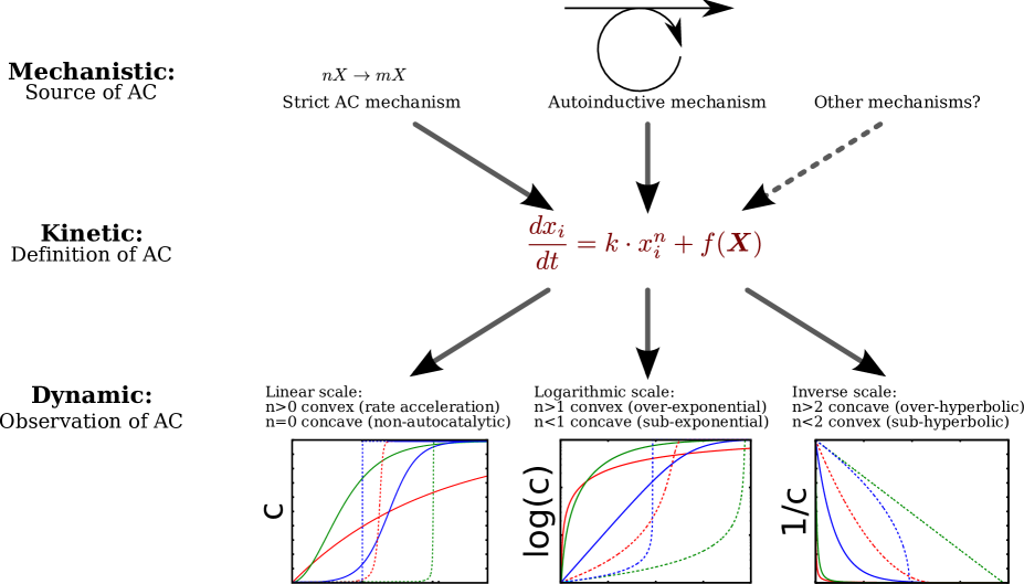
Figure 1: Classification of the concepts of autocatalysis (AC) depending on their descriptions (mechanistic, kinetic, and dynamic). The graphs represents the time evolution of a non-autocatalytic reaction ($n=0$, red), and of autocatalytic reactions of order $n=1/2$ (green), $1$ (blue), $3/2$ (dotted red), $2$ (dotted green), and $3$ (dotted blue).

2 Autocatalysis: a Practical Definition

2.1 A Kinetic Signature

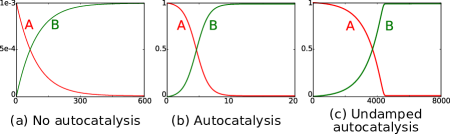
Figure 2: (a-b): First order autocatalytic process ($\Gamma_{1}=10^{2}$ M.s^-1) in presence of a non-autocatalytic reaction ($\Gamma_{2}=10^{-2}$ M.s^-1) of spontaneous transformation of A into B ($K_{A}=1$ M, $K_{B}=10^{2}$ M). (a) Diluted ($a_{o}=10^{-3}$ M). (b) Concentrated ($a_{0}=1$ M). (c) Undamped autocatalysis (Indirect autocatalysis, described in fig. 4(b), $\Gamma_{4}=0.1$ M.s^-1)

From its origin, the notion of autocatalysis has focused on the kinetic pattern of the chemical evolution [3]. The general definition of autocatalysis as a chemical process in which one of the products catalyzes its own formation can be mathematically generalized as:

$$\dfrac{\operatorname{d\!}{}x_{i}}{\operatorname{d\!}{t}}=k(\mathbf{X})\cdot x_{i}^{n}+f(\mathbf{X}),\quad k>0;\leavevmode\nobreak\ n>0;\leavevmode\nobreak\ |k|\gg|f|$$ (1)

$\mathbf{X}$ is the vector of all the concentrations $x_{j}$. An autocatalysis for the compound $x_{i}$ exists when the conditions of eq. 1 are fulfilled. The term $k(\mathbf{X})\cdot x_{i}^{n}$ describes the autocatalytic process itself, while $f(\mathbf{X})$ describes the sum of all other contributions coming from the rest of the chemical system.

We have an effective practical definition of the concept of autocatalysis, based on a precise mathematical formulation. The causes of this kinetic signature can be investigated, searching what mechanism is responsible for the autocatalytic term. This leads to the discovery of a series of different kinds of autocatalysis processes, and their respective effect, describing what observable behavior is generated by the autocatalytic term (see fig. 1).

2.2 Potential vs Effective Autocatalysis

This kinetic definition is purely structural. As a matter of fact, a system may contain potential autocatalysis i.e. an autocatalytic core exists in the reaction network. However, in the absence of some specific conditions necessary for this autocatalysis to be effective, the potential autocatalysis may be hidden by other kinetic effects, and thus not manifests its behavior in practice.

Possibly, in eq. 1, the term $f(\boldsymbol{X})$ may simply overwhelm the autocatalytic process. This is typically the case when an autocatalysis is present together with the non-catalyzed version of the same reaction, that may not be negligible in all conditions. A simple example is a system simultaneously containing a direct autocatalysis $A$ + $B$ -> 2$B$, concurrent with the non autocatalytic reaction $A$ -> $B$. The autocatalytic process follows a bimolecular kinetics, and will be more efficient in a concentrated than in a diluted solution. The dynamic profile of the reaction is thus sigmoidal for high initial concentration of $A$, but no more for low initial concentration (see fig. 2(a-b)).

It can also be seen that the term $k(\boldsymbol{X})$ may vary during the reaction process. In a simple autocatalytic process as described above, $k$ is proportional to the concentration in $A$, and is thus more important at the beginning of the reaction (thus an initial exponential increase of the product $B$) that at the end (thus a damping of the autocatalysis) resulting in a global sigmoidal evolution. In systems were the influence of $A$ on $k$ is weaker, as detailed further, an undamped autocatalysis will be observed characterized by an exponential variation until the very end (see fig. 2(c)).

3 Mechanistic Distinctions

How can this kinetic pattern be realized? Let us now detail several types of mechanisms. They can all be reduced, in some conditions, to the autocatalysis kinetic pattern of eq. 1. All of them will be equally defined in the paper as autocatalytic, while this status may have been disputed in the past on account of the distinct chemical realisations. In the following, we emphasize the major mechanistic pattern to eventually be reduced to an equivalent kinetic autocatalysis, and discuss where their difference comes from.

3.1 Template Autocatalysis

The simplest autocatalysis is obtained by the $X$ -> 2$X$ pattern. It can be represented by:

$$\ce{A+B<=>[k_{1}][k_{-1}]B+B}$$ (2)

The corresponding network is given in fig. 3(a). It can further be decomposed through the introduction of an intermediate compound $C$:

$$\ce{$A$+$B$} \ce{<=>[\Gamma_{1}]C}$$ (3)

$$\ce{C} \ce{<=>[\Gamma_{2}]$B$+$B$}$$ (4)

The corresponding network is given in fig. 3(b).

The first mechanism entails the following kinetic evolution:

$$\mathinner{\dfrac{\operatorname{d\!}{}b}{\operatorname{d\!}{t}}} =-\mathinner{\dfrac{\operatorname{d\!}{}a}{\operatorname{d\!}{t}}}$$ (5)

$$=k_{1}ab-k_{-1}b^{2}$$ (6)

This can be expressed as a chemical flux $\varphi=\dfrac{\operatorname{d\!}{}b}{\operatorname{d\!}{t}}$, by relying on the Mikulecky formalism [18, 19, 20]:

$$\varphi =\Gamma_{1}(V_{A}V_{B}-V_{B}^{2})$$ (7)

$$V_{A} =\frac{a}{K_{A}}$$ (8)

$$V_{B} =\frac{b}{K_{B}}$$ (9)

$$\Gamma_{1} =k_{1}\cdot K_{A}K_{B}=k_{-1}\cdot K_{B}^{2}$$ (10)

$k_{1}$ and $k_{-1}$ are the kinetic constant rates of the reaction $1$ in the direct and reverse direction. $K_{A}$ and $K_{B}$ are the thermodynamic constant of formation of compounds $A$ and $B$.

Formally there is a linear flux $\varphi$ of transformation of $A$ into $B$, coupled to a circular flux of same intensity from $B$ back to $B$ (see fig. 3(a-b)). In presence of an intermediate compound, the equations becomes:

$$\varphi_{1} =\Gamma_{1}(V_{A}V_{B}-V_{C})$$ (11)

$$\varphi_{2} =\Gamma_{2}(V_{C}-V_{B}^{2})$$ (12)

Under the hypothesis that $C$ is an unstable intermediate, (i.e. $K_{C}\ll K_{B},K_{A}$), the variation of $C$ can be neglected compared to the variations of $A$ and $B$ (quasi steady-state approximation, hereafter QSSA), so that:

$$\varphi_{1} \simeq\varphi_{2}$$ (13)

$$=\varphi$$ (14)

$$\Rightarrow\quad\varphi =\frac{\Gamma_{1}\Gamma_{2}}{\Gamma_{1}+\Gamma_{2}}(V_{A}V_{B}-V_{B}^{2})$$ (15)

The system is strictly equivalent to the direct autocatalysis, with an apparent rate ${\Gamma_{1}\Gamma_{2}}/(\Gamma_{1}+\Gamma_{2})$. With these two systems, we are in presence of the perfect kinetic signature of an autocatalytic system, following a sigmoidal evolution (see fig. 4(a)). This equivalence is guaranteed as long as the compound $C$ remains unstable. When it is not the case, the dimeric intermediate $C$ hardly liberates the final compound $B$, which eventually leads to an autocatalytic process of order $1/2$ rather than $1$ [21, 22].

Template autocatalysis requires a direct association between the reactants and the products. This is typically the case of DNA replication, one double strand molecule giving birth to two identical double strand molecules, thanks to the very selective association of complementary nucleotides along each strand. More simple examples can be found in some biological mechanisms that requires autocatalytic processes, for example for the generation of chemical oscillation inducing circadian rhytmicity in cells. The system described by Mehra et al[23] is based on a non equilibrium system of association/dissociation of proteins forming a large chemical cycle [$C$ -> $AC$ -> $AC^{*}$ -> $ABC^{*}$ -> $BC^{*}$ -> $C^{*}$ -> $C$], maintained by a flux of ATP consumption, one cycle consuming and freeing $A$ and $B$[23]. The oscillations are generated by coupling this chemical flux to an autocatalytic process of phosphorylation obeying to the reaction scheme[24]: $A$ + $C$ + $AC^{*}$ -> 2$AC^{*}$.

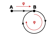
(a) Direct

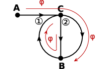
(b) Direct with intermediate

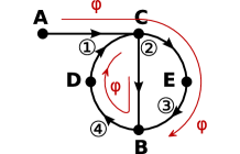
(c) Indirect

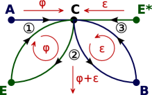
(d) Autoinductive

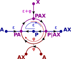
(e) Iwamura et al[25] system

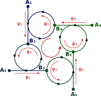
(f) Collective

Figure 3: Reaction network of different autocatalytic processes of spontaneous transformation of $A$ into $B$ (a-d), of $A+X$ into $AX$ (e), and of $A_{i}$ into $B_{i}$ (f). The indicated fluxes correspond to what is observed within the QSSA.

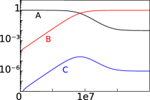
(a) Direct

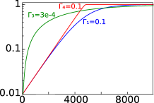
(b) Indirect

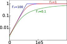
(c) Autoinductive

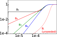
(d) Collective

Figure 4: Time evolution of compound concentrations for different autocatalytic processes of spontaneous transformation of $A$ into $B$ ($K_{A}=1$ M and $K_{B}=100$ M) in a logarithmic scale for concentrations (a-c), or logarithmic scales for both time and concentrations (d). $K$ and concentrations are in M, times in s, and $\Gamma$ in M.s^-1. (a): fig. 3(b), $\Gamma_{1}=1$, $\Gamma_{2}=10^{-4}$, $K_{C}=0.01$; (b): fig. 3(c), $\Gamma_{1}=\Gamma_{2}=\Gamma_{3}=\Gamma_{4}=10$ (except the values indicated on the graph), $K_{C}=K_{D}=K_{E}=0.01$; (c): fig. 3(d), $\Gamma_{2}=\Gamma_{3}=100$, $K_{C}=K_{E}=1$, $K_{E^{*}}=10$; (d): fig. 3(f), $\Gamma_{1}=100$, $\Gamma_{2}=1$.

3.2 Network Autocatalysis

The direct mechanism of template autocatalysis is conceptually the simplest framework. It may actually not be the most representative class of autocatalysis, and a similar kinetic signature can result from more complex reaction networks.

3.2.1 Indirect Autocatalysis:

The autocatalytic effect can be indirect when reactant and products never directly interact:

$$A+D \ce{<=>[\Gamma_{1}]$C$}$$ (16)

$$C \ce{<=>[\Gamma_{2}]}B+E$$ (17)

$$E \ce{<=>[\Gamma_{3}]}B$$ (18)

$$B \ce{<=>[\Gamma_{4}]}D$$ (19)

There is no direct $A/B$ coupling, nor direct $2B$ formation, but the presence of a dimeric compound $C$. The network decomposition of this system (see fig. 3(c)) implies once again a linear flux of transformation of $A$ into $B$, linked to a large cycle of reaction transforming $B$ back to $B$. This system is still reducible to an $X$ -> 2$X$ pattern.

The QSSA for compounds $C,D,E$ allows to express the reaction flux as:

$$\varphi =\frac{1}{\frac{1}{\Gamma_{1}}+\frac{1}{\Gamma_{2}}+\frac{V_{A}}{\Gamma_{4}}+\frac{V_{B}}{\Gamma_{3}}}\left(V_{A}V_{B}-V_{B}^{2}\right)$$ (20)

The details of the calculations are given in appendix.

When the terms $V_{A}/\Gamma_{4}$ and $V_{B}/\Gamma_{3}$ are small compared to either $\Gamma_{1}^{-1}$ or $\Gamma_{2}^{-1}$ (i.e. when at least one of the two reactions of eq. 16-eq. 17) is kinetically limiting), the system behaves like a simple autocatalytic system, with $\varphi\propto a\cdot b$ before the reaction completion, with a progressive damping of the exponential growth as long as $A$ is consumed. When the term $V_{A}/\Gamma_{4}$ is predominant (i.e when the reaction of eq. 19 is kinetically limiting), the flux is $\varphi\propto b$: the profile remains exponential up to the reaction completion, with no damping due to $A$ consumption. When the term $V_{B}/\Gamma_{3}$ is predominant (i.e when the reaction of eq. 18 is kinetically limiting), the flux is $\varphi\propto a$: the autocatalytic effect is lost (see fig. 4(b)).

Network autocatalysis is probably the most common kind of mechanisms. A typical biochemical example is the presence of autocatalysis in glycolysis [26, 27]. In this system, there is a net balance following the $X$ -> 2$X$ pattern. ATP must be consumed to initiate the degradation of glucose, but much more molecules of ATP are produced during the whole process. While these systems are effectively autocatalytic, there is obviously no possible “templating” effect of one molecule of ATP to generate another one.

3.2.2 Collective Autocatalysis:

More general systems, reminiscent of the Eigen’s hypercycles [28], are responsible of even more indirect autocatalysis. No compound influences its own formation rate, but rather influences the formation of other compounds, which in turn influence other reactions, in such a way that the whole set of compounds collectively catalyzes its own formation.

A simple framework can be built from the association of several systems of transformation $A_{i}$ -> $B_{i}$, each $B_{i}$ catalyzing the next reaction (see fig. 3(f)):

$$A_{i}+B_{i-1} \ce{<=>[\Gamma_{i}]}B_{i}+B_{i-1}$$ (21)

$$(\mathrm{with}\leavevmode\nobreak\ i=\{1,2,3,4\}\leavevmode\nobreak\ \mathrm{and}\leavevmode\nobreak\ B_{4}\equiv B_{0})$$

There are four independent systems, only connected by catalytic activities.

If the system is totally symmetric, then all $b_{i}$ are equal, and all $a_{i}$ are equal, so that the rates become:

$$\varphi_{i} =\Gamma_{i}V_{B_{i-1}}(V_{A_{i}}-V_{B_{i}})$$ (22)

$$\varphi =\Gamma V_{B}(V_{A}-V_{B})$$ (23)

This leads to a collective autocatalysis with all compounds present. They mutually favor their formation, which results in an exponential growth of each compound (see fig. 4(d) dotted curve).

With symmetrical initial conditions (i.e. identical for the four systems), the system strictly behaves autocatalytically. If the symmetry is broken, e.g. by seeding only one of the $B_{i}$, the system acts with delays. The evolution laws are sub-exponential, of increasing order; at the very beginning of the reaction, considering that $A_{i}$ do not significantly change and that $B_{i}$ are in low concentrations, we obtain $\varphi_{i}\propto t^{i-1}$. Seeding with $B_{1}$, the compound $B_{2}$ evolves in $t^{2}$. Its impact on compound $B_{3}$ induces an evolution in $t^{3}$. In its turn, the impact of compound $B_{3}$ on compound $B_{4}$ induces an evolution in $t^{4}$. The compound $1$ at first remains constant, and it is only following a given delay that it gets catalyzed by $B_{4}$ (see fig. 4(d)).

This system is actually not characterized by a direct cyclic flux, but by a cycle of fluxes influencing each other and resulting in a cooperative collective effect:

$$(A_{1}+A_{2}+A_{3}+A_{4})+(B_{1}+B_{2}+B_{3}+B_{4})$$ (24)

$$\ce{->}\quad 2(B_{1}+B_{2}+B_{3}+B_{4})$$ (25)

The simultaneous presence of all different compounds is needed to observe a first order autocatalytic effect. Given asymmetric initial conditions, a transitory evolution of lower order is first observed, until the formation of the full set of compounds.

A typical example of collective autocatalysis is observed for the replication of viroids [29]. Each opposite strand of cyclic RNAs can catalyze the formation of the other one, leading to the global growth of the viroid RNA in the infected cell.

3.2.3 Template vs Network Autocatalysis:

All the preceding systems can be reduced to a $X$ -> 2$X$ pattern. This is characterized by a linear flux of chemical transformations, coupled to an internal loop flux: for each molecule (or set of molecules) $A$ transformed into $B$, one $B$ is transformed and goes back to $B$, following a more or less complex pathways. They can be considered as mechanistically equivalent: a seemingly direct autocatalysis may really be an indirect autocatalysis once its precise mechanism is known, decomposing the global reaction into several elementary reactions.

Practically, autocatalysis will be considered to be direct (or template) when a dimeric complex of the product is formed (i.e. allowing the “imprint” of the product onto the reactant). If such template complex is never formed, we preferentially speak of network autocatalysis, in which the $X$ -> 2$X$ pattern only results from the reaction balance.

3.3 Autoinductive Autocatalysis

Some reactions are not characterized by a $X$ -> 2$X$ pattern, but still exhibit a mechanism for the enhancement of the reaction rate by the products. This is typically the case for systems where the products increase the reactivity of the reaction catalyst rather than directly influencing their reaction production itself. These systems still possess the kinetic signature of eq. 1, but are sometime referred as “autoinductive” instead of “autocatalytic” [17].

3.3.1 Simple network:

Let us take a simple reaction network of a transformation $A$ -> $B$ catalyzed by a compound that can exist under two forms $E/E^{*}$, $E^{*}$ being the more stable one. These two forms of the catalyst interact differently with the product $B$ (see fig. 3(d)):

$$A+E \ce{<=>[\Gamma_{1}]}C$$ (26)

$$C \ce{<=>[\Gamma_{2}]}B+E$$ (27)

$$C \ce{<=>[\Gamma_{3}]}B+E^{*}$$ (28)

There is no dimeric compound in the system, even indirectly formed.

Provided the catalyst, present in $C$, $E$, and $E^{*}$, is in low total concentration, the QSSA implies the presence of two fluxes: the transformation of $A$ into $B$ catalyzed by $E$ of intensity $\varphi$, and the transformation of $E^{*}$ into $E$ catalyzed by $B$ of intensity $\varepsilon$, with $\varphi\gg\varepsilon$. Assuming that $E^{*}$ is very stable compared to $E$ and $C$, this decomposition gives (see appendix for details):

$$\varphi =\frac{\Gamma_{1}\Gamma_{2}V_{E^{*}}^{0}}{\Gamma_{1}V_{A}+\Gamma_{2}V_{B}}(V_{B}V_{A}-V_{B}^{2})$$ (29)

The autoinduction is kinetically equivalent to the indirect autocatalysis mechanism:

• When $\Gamma_{2}\gg\Gamma_{1}\frac{K_{B}}{K_{A}}$, the flux $\varphi$ is $\Gamma_{1}V_{E^{*}}^{0}(V_{A}-V_{B})$: the system is non-autocatalytic.

• When $\Gamma_{2}\approx\Gamma_{1}\frac{K_{B}}{K_{A}}$, the flux $\varphi$ is $\Gamma_{2}\frac{V_{E^{*}}^{0}}{V_{A}^{0}}(V_{A}V_{B}-V_{B}^{2})$: the system is simply autocatalytic.

• When $\Gamma_{2}\ll\Gamma_{1}\frac{K_{B}}{K_{A}}$ , the flux $\varphi$ is $\Gamma_{2}V_{E^{*}}^{0}\left(V_{B}-\frac{V_{B}^{2}}{V_{A}}\right)$: the system presents an undamped autocatalysis.

Following the kinetic analysis, the behavior is similar to the time evolution of autocatalytic systems (See fig. 4(c)). The behavioral equivalence of these two systems (kinetically equivalent but mechanistically very different) will be investigated in more details in the next section.

3.3.2 Iwamura’s model

An example of autoinductive autocatalysis is the proline-catalyzed $\alpha$-aminoxylation of aldehydes[25]. The core principle is a reaction $A$ + $X$ -> $AX$, catalyzed by $P$, the product $AX$ catalyzing the first catalytic step $P$ + $A$ -> $PA$ (see fig. 3(e)). This chemical system can be decomposed into two different fluxes $A$ + $X$ -> $AX$, one coupled to a catalytic cycle [$P$ -> $PA$ -> $PAX$ -> $P|AX$ -> $P$], and one coupled to a catalytic cycle [$PA$ -> $PAX$ -> $P|AX$ -> $PA$]. The first one contains the slow reaction of $A$ on $P$, and corresponds to a slow flux $\varepsilon$. The second one only contains fast reactions, and corresponds to a fast flux $\varphi$. In an ideal case (see appendix for details), the flux of production of $AX$ is equal to:

$$\varphi=\Gamma_{5}V_{P}^{0}\left(V_{A}V_{AX}-\frac{V_{AX}^{2}}{V_{X}}\right)$$ (30)

The kinetic signature of an undamped autocatalysis is once again obtained.

3.3.3 Network vs Autoinductive Autocatalysis:

Autoinductive autocatalysis is mechanistically different from network or template autocatalysis. The balance equation is rather of the form $A$ + $\alpha$ $B$ -> $(1+\alpha)$ $B$, with $\alpha\ll 1$. The linear transformation $A$ -> $B$ is only weakly coupled to the cycle of $B$ back to itself, this latter one being subject to a much lower flux than the linear flux. However, autoinduction is kinetically and dynamically equivalent to network autocatalysis, leading to the same kind of differential equation, and thus of behavior. It must be noted that the undamped exponential profile—due to a flux only proportional to the products and not to the reactant—is not characteristic of autoinductive processes [25] but can also be explained by network autocatalytic mechanisms, when the consumption of the reactant is not limiting the kinetic of the network.

4 Embedded Autocatalyses

Autocatalysis is not so important per se but as a way of giving birth to rich non-linear behaviors like bifurcation, multistability or chemical oscillations. It is crucial to study the interaction of autocatalytic mechanisms and their ability to generate such behaviors when embedded in a larger chemical network.

4.1 Dynamical Distinctions

Different behaviors depending on the order $n$ of the autocatalysis can be observed in biochemical competitive systems. They are classically studied in population evolution [30, 31] and described as “survival of the all” in the case of $0<n<1$ (characterized by the coexistence of all compounds), as “survival of the fittest” in the case of $n=1$ (when the only stable solution retains the fittest compound or the most "reproductible") and as “survival of the first” in the case of $n>1$ (when the final solution just retains the product initially present in the highest concentration).

The case $0<n<1$ is the least interesting one, as it hardly leads to a clear selectionnist process. However, real mechanism that seems to possess a first order autocatalysis may actually present a lower autocatalytic order. This is typically the case for direct template autocatalysis, in which the order falls to $1/2$ on account of the high stability of the dimeric intermediate—which is actually a necessary condition for the selectivity of template replication [32, 21, 22]. This turns out to be a fundamental problem for understanding the emergence of the first replicative molecules [33, 34, 35].

More complex mechanisms may lead to higher orders, typically by the formation of dimeric autocatalysts [36]. This is the case of the Soai reaction whose high sensitivity to initial conditions may potentially be explained by the formation of trimeric [37] or even hexameric complexes [38].

4.2 Comparative Efficiency of Direct and Autoinductive Autocatalyses

The relative efficiency of two different autocatalytic mechanisms can be evaluated by having them competing which each other. Bifurcations appear when these two autocatalytic processes are placed in a nonequilibrium open-flow system, both being fed by the same incoming compound and with cross-inhibition between them:

$$\ce{->}A$$ (incoming flux) (31)

$$A \ce{<=>[\alpha]}B_{1}$$ (Direct AC) (32)

$$A \ce{<=>[\beta]}B_{2}$$ (Autoinduced AC) (33)

$$B_{1}+B_{2} \ce{->}(P)$$ (cross inhibition) (34)

$$B_{1} \ce{->}$$ (outgoing flux) (35)

$$B_{2} \ce{->}$$ (outgoing flux) (36)

In the case of total symmetry between $B_{1}$ and $B_{2}$, with the same direct autocatalystic mechanism, this system would correspond to the classical Frank model for the emergence of homochirality [12]. Because of the system symmetry, the same probability to end up with either $B_{1}$ or $B_{2}$ is observed.

The kinetic equivalence between template autocatalysis and autoinductive autocatalysis can be shown by making these two mechanisms to compete, replacing eq. 32 and eq. 33 by the corresponding mechanism. Kinetic parameters have first been normalized so that each reaction leads on their own to the same kinetic behavior (sigmoidal evolution, half-reaction at $10^{5}$ s), and then multiplied by respectively $\alpha$ and $\beta$ parameters in order to tune the respective velocity of each mechanism. The result is actually symmetrical between the two processes and only the fastest product is maintained in the system: $B_{1}$ when $\alpha>\beta$, and $B_{2}$ when $\alpha<\beta$ (see fig. 5(a)). As a consequence, while mechanistically different, these two autocatalysis are shown to be dynamically equivalent.

This selectivity is independent of the relative stability of $B_{1}$ and $B_{2}$, but is only possible for kinetics that are well adapted to the global influx of matter. For slow kinetics, there is a flush of the system, and neither $B_{1}$ nor $B_{2}$ can be maintained. For fast kinetics, the system is close to equilibrium, the compounds $B_{1}$ and $B_{2}$ being both present in proportion to their respective stability (see fig. 5(b)). Such result is well known for open flow Frank systems [39].

(a) Sharp bifurcation depending on the relative values of $\alpha$ and $\beta$ for moderate reactivities.

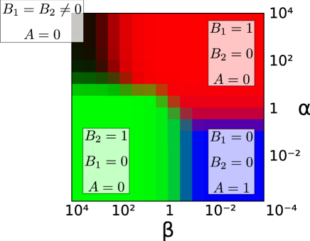
(b) Different zones of behaviors: majority of $A$ for $\alpha,\beta\ll 1$, majority of $B_{1}$ for $\alpha>\beta$, majority of $B_{2}$ for $\alpha<\beta$, and coexistence of $B_{1}$ and $B_{2}$ for $\alpha,\beta\gg 1$.

Figure 5: Competition between template and autoinductive autocatalysis, generating respectively $B_{1}$ and $B_{2}$ compounds from the same $A$ compound. Incoming flux of $A$, and outgoing fluxes of $B_{1}$ and $B_{2}$, $10^{-5}$ M.s^-1. $K_{A}=1$, $K_{B_{1}}=K_{B_{2}}=100$. Direct autocatalysis: $\Gamma_{AC}=10^{-2}\cdot\alpha$, $\Gamma_{NC}=10^{-6}\cdot\alpha$. Autoinduction, according to fig. 3(d): $\Gamma_{1}=\beta$, $\Gamma_{2}=\Gamma_{3}=100\cdot\beta$, $K_{C}=K_{E}=1$; $K_{E^{*}}=10$.

4.3 From Autocatalytic Processes towards Autocatalytic Sets

These competitive systems are able to dynamically maintain a set of components, to the detriment of others. These autocatalytic networks must however not be confused with autocatalytic sets. This latter notion is rather popular in the artificial life literature, but relies much more on the cooperation between autocatalytic mechanisms than on the competition that has just been detailed here. This implies a notion of material closure of the system and of self maintenance of the whole network by crossing energetical fluxes[40, 41, 42]. Confusion among these different phenomena can be pinpointed in the literature [17], when the failure of autoinductive sets to be maintained do not originate from a difference of behavior between autocatalytic and autoinductive mechanisms, but from a defect in the closure of the system (e.g. induced by the leakage of some components).

5 Conclusion

Important distinctions need to be made between mechanistic and dynamic aspects of autocatalysis. One single mechanism can produce different dynamics, while identical dynamics can originate from different mechanisms. Thus, a pragmatic definition of autocatalysis have to be based on a kinetic signature, in order to classify the systems according their observable behavior, rather than on a mechanistic signature, that would instead classify the systems according to the origin of their behavior. All the different autocatalytic processes described in this work are able to generate autocatalytic kinetics. They can constitute a pathway towards the onset of “self-sustaining autocatalytic sets”, as chemical attractor in non-equilibrium networks. However, the problem of the evolvability of such systems must be kept in mind [43]. If a system evolves towards a stable attractor, no evolution turns out to be possible. There is the necessity of “open-ended” evolution [44] i.e. the possibility for a dynamic set to not only maintain itself (i.e. as a strict autocatalytic system) but also to act as a “general autocatalytic set”, redounding upon the concept originally introduced by Muller[8] for the autocatalytic power linked to mutability of genes. For example, insights can be gained by a deeper and renewed study of the evolution of prions as a simple mechanism of mutable autocatalytic systems [45].

6 Appendix

The kinetic behavior of three different mechanisms for autocatalytic transformations have been studied in details. The methodology consists in establishing the different chemical fluxes of the network. The relationship between these fluxes can be simplified by assuming the QSSA for relevant compounds. The purpose is then to establish the expression of the transformation flux $\varphi$ as a function of the concentration of the reactants and the products.

6.1 Indirect autocatalysis

The four fluxes of fig. 3(c) can be written as:

$$\varphi_{1} =\Gamma_{1}(V_{A}V_{D}-V_{C})$$ (37)

$$\varphi_{2} =\Gamma_{2}(V_{C}-V_{B}V_{E})$$ (38)

$$\varphi_{3} =\Gamma_{3}(V_{E}-V_{B})$$ (39)

$$\varphi_{4} =\Gamma_{4}(V_{B}-V_{D})$$ (40)

The QSSA for $D$ comes down to $\varphi_{1}\simeq\varphi_{4}$:

$$\Gamma_{1}V_{A}V_{D}-\Gamma_{1}V_{C} =\Gamma_{4}V_{B}-\Gamma_{4}V_{D}$$ (41)

$$(\Gamma_{1}V_{A}+\Gamma_{4})V_{D} =\Gamma_{4}V_{B}+\Gamma_{1}V_{C}$$ (42)

$$V_{D} =\frac{\Gamma_{4}V_{B}+\Gamma_{1}V_{C}}{\Gamma_{1}V_{A}+\Gamma_{4}}$$ (43)

Replacing $V_{D}$ by eq. 43 in eq. 37 gives:

$$\varphi_{1} =\Gamma_{1}\left(V_{A}\frac{\Gamma_{4}V_{B}+\Gamma_{1}V_{C}}{\Gamma_{1}V_{A}+\Gamma_{4}}-V_{C})\right)$$ (44)

$$=\frac{\Gamma_{1}\Gamma_{4}}{\Gamma_{1}V_{A}+\Gamma_{4}}V_{A}V_{B}+\Gamma_{1}V_{C}\frac{-\Gamma_{4}}{\Gamma_{1}V_{A}+\Gamma_{4}}$$ (45)

$$=\frac{\Gamma_{1}\Gamma_{4}}{\Gamma_{1}V_{A}+\Gamma_{4}}(V_{A}V_{B}-V_{C})$$ (46)

The QSSA for $E$ comes down to $\varphi_{2}\simeq\varphi_{3}$:

$$\Gamma_{2}V_{C}-\Gamma_{2}V_{B}V_{E} =\Gamma_{3}V_{E}-\Gamma_{3}V_{B}$$ (47)

$$V_{E} =\frac{\Gamma_{2}V_{C}+\Gamma_{3}V_{B}}{\Gamma_{3}+\Gamma_{2}V_{B}}$$ (48)

Replacing $V_{E}$ by eq. 48 in eq. 38 by Eq.gives:

$$\varphi_{2} =\Gamma_{2}\left(V_{C}-V_{B}\frac{\Gamma_{2}V_{C}+\Gamma_{3}V_{B}}{\Gamma_{3}+\Gamma_{2}V_{B}}\right)$$ (49)

$$=\Gamma_{2}V_{C}\frac{\Gamma_{3}}{\Gamma_{3}+\Gamma_{2}V_{B}}-\Gamma_{2}V_{B}\frac{\Gamma_{3}V_{B}}{\Gamma_{3}+\Gamma_{2}V_{B}}$$ (50)

$$=\frac{\Gamma_{2}\Gamma_{3}}{\Gamma_{3}+\Gamma_{2}V_{B}}(V_{C}-V_{B}^{2})$$ (51)

At last, the QSSA for $C$ comes down to $\varphi_{1}\simeq\varphi_{2}=\varphi$. Combining eq. 46 and Eq, eq. 51 gives:

$$V_{C} =\frac{\Gamma^{\prime}_{1}V_{A}V_{B}+\Gamma^{\prime}_{2}V_{B}^{2}}{\Gamma^{\prime}_{1}+\Gamma^{\prime}_{2}}$$ (52)

$$\mathrm{with}\qquad\Gamma^{\prime}_{1} =\frac{\Gamma_{1}\Gamma_{4}}{\Gamma_{1}V_{A}+\Gamma_{4}}$$ (53)

$$\mathrm{and}\qquad\Gamma^{\prime}_{2} =\frac{\Gamma_{2}\Gamma_{3}}{\Gamma_{3}+\Gamma_{2}V_{B}}$$ (54)

Replacing $V_{C}$ by eq. 52 in eq. 46 gives:

$$\varphi =\Gamma^{\prime}_{1}V_{A}V_{B}-\Gamma^{\prime}_{1}\frac{\Gamma^{\prime}_{1}V_{A}V_{B}+\Gamma^{\prime}_{2}V_{B}^{2}}{\Gamma^{\prime}_{1}+\Gamma^{\prime}_{2}}$$ (55)

$$=\left(\Gamma^{\prime}_{1}-\frac{\Gamma^{\prime 2}_{1}}{\Gamma^{\prime}_{1}+\Gamma^{\prime}_{2}}\right)V_{A}V_{B}-\frac{\Gamma^{\prime}_{1}\Gamma^{\prime}_{2}}{\Gamma^{\prime}_{1}+\Gamma^{\prime}_{2}}V_{B}^{2}$$ (56)

$$=\frac{\Gamma^{\prime}_{1}\Gamma^{\prime}_{2}}{\Gamma^{\prime}_{1}+\Gamma^{\prime}_{2}}(V_{A}V_{B}-V_{B}^{2})$$ (57)

Replacing $\Gamma^{\prime}_{1}$ and $\Gamma^{\prime}_{2}$ by their expression given in eq. 53 and eq. 54 then gives:

$$\varphi =\frac{V_{A}V_{B}-V_{B}^{2}}{\frac{1}{\Gamma_{1}}+\frac{1}{\Gamma_{2}}+\frac{V_{A}}{\Gamma_{4}}+\frac{V_{B}}{\Gamma_{3}}}$$ (58)

6.2 Autoinductive autocatalysis

The three fluxes of fig. 3(d) are:

$$\varphi_{1} =\Gamma_{1}(V_{A}V_{E}-V_{C})$$ (59)

$$\varphi_{2} =\Gamma_{2}(V_{C}-V_{B}V_{E})$$ (60)

$$\varphi_{3} =\Gamma_{3}(V_{B}V_{E^{*}}-V_{C})$$ (61)

The QSSA for $C$ comes down to $\varphi_{1}+\varphi_{3}\simeq\varphi_{2}$, and the QSSA for $E$ comes down to $\varphi_{1}\simeq\varphi_{2}$. This implies that $\varphi_{3}\ll\varphi_{1}$, so that with $\varphi_{3}=\varepsilon$ and, $\varphi_{1}=\varphi$, we obtain:

$$\varphi_{2} =\varphi+\varepsilon\simeq\varphi$$ (62)

In that context, eq. 61 gives:

$$V_{C} =V_{B}V_{E^{*}}-\frac{\varepsilon}{\Gamma_{3}}$$ (63)

Combining eq. 59, eq. 60 in eq. 62 then gives:

$$\Gamma_{2}V_{C}-\Gamma_{2}V_{B}V_{E} =\Gamma_{1}V_{A}V_{E}-\Gamma_{1}V_{C}+\varepsilon$$ (64)

$$V_{E} =\frac{(\Gamma_{1}+\Gamma_{2})V_{C}-\varepsilon}{\Gamma_{1}V_{A}+\Gamma_{2}V_{B}}$$ (65)

Replacing $V_{C}$ by its value given in eq. 63 leads to:

$$V_{E} =\frac{(\Gamma_{1}+\Gamma_{2})V_{E^{*}}V_{B}-\frac{\Gamma_{1}+\Gamma_{2}+\Gamma_{3}}{\Gamma_{3}}\varepsilon}{\Gamma_{1}V_{A}+\Gamma_{2}V_{B}}$$ (66)

$$V_{E} \simeq\frac{(\Gamma_{1}+\Gamma_{2})V_{E^{*}}V_{B}}{\Gamma_{1}V_{A}+\Gamma_{2}V_{B}}$$ (67)

The flux of destruction of $A$ can be computed by replacing $V_{E}$ in eq. 59 by eq. 67 (computing the flux of formation of $B$ from eq. 60 would of course give the same result):

$$\varphi =\Gamma_{1}\left(V_{A}\frac{(\Gamma_{1}+\Gamma_{2})V_{E^{*}}V_{B}}{\Gamma_{1}V_{A}+\Gamma_{2}V_{B}}-V_{B}V_{E^{*}}\right)$$ (68)

$$=\Gamma_{1}\frac{(\Gamma_{1}+\Gamma_{2})V_{E^{*}}V_{B}V_{A}-V_{B}V_{E^{*}}(\Gamma_{1}V_{A}+\Gamma_{2}V_{B})}{\Gamma_{1}V_{A}+\Gamma_{2}V_{B}}$$ (69)

$$=\Gamma_{1}\Gamma_{2}V_{E^{*}}\frac{V_{B}V_{A}-V_{B}^{2}}{\Gamma_{1}V_{A}+\Gamma_{2}V_{B}}$$ (70)

The law of conservation of $E$ compounds leads to:

$$\varphi =\frac{\Gamma_{1}\Gamma_{2}V_{E^{*}}^{0}(V_{B}V_{A}-V_{B}^{2})}{(\Gamma_{1}V_{A}+\Gamma_{2}V_{B})(1+r_{C}V_{C}+r_{E}V_{E})}$$ (71)

with $r_{C}=K_{C}/K_{E^{*}}$ and $r_{E}=K_{E}/K_{E^{*}}$. Assuming that $E^{*}$ is the much more stable than $C$ and $E$, $r_{C}$ and $r_{E}\ll 1$, so that we finally obtain:

$$\varphi =\frac{\Gamma_{1}\Gamma_{2}V_{E^{*}}^{0}}{\Gamma_{1}V_{A}+\Gamma_{2}V_{B}}(V_{B}V_{A}-V_{B}^{2})$$ (72)

6.3 Iwamura’s model

The five fluxes of fig. 3(e) are:

$$\varphi_{1} =\Gamma_{1}(V_{A}V_{P}-V_{PA})$$ (73)

$$\varphi_{2} =\Gamma_{2}(V_{PA}V_{X}-V_{PAX})$$ (74)

$$\varphi_{3} =\Gamma_{3}(V_{PAX}-V_{P|AX})$$ (75)

$$\varphi_{4} =\Gamma_{4}(V_{P|AX}-V_{P}V_{AX})$$ (76)

$$\varphi_{5} =\Gamma_{5}(V_{P|AX}V_{A}-V_{PA}V_{AX})$$ (77)

The QSSA for $P$ leads to $\varphi_{1}=\varphi_{4}$; for $PA$, it leads to $\varphi_{2}=\varphi_{1}+\varphi 5$; for $PAX$ it leads to $\varphi_{3}=\varphi_{2}$; for $P|AX$, it leads to $\varphi_{3}=\varphi_{4}+\varphi_{5}$. The fluxes can thus be decomposed into two elementary fluxes:

$$\varphi_{1} =\varepsilon$$ (78)

$$\varphi_{2} =\varphi+\varepsilon$$ (79)

$$\varphi_{3} =\varphi+\varepsilon$$ (80)

$$\varphi_{4} =\varepsilon$$ (81)

$$\varphi_{5} =\varphi$$ (82)

$\varphi$ is the flux of the catalytic reaction, and $\varepsilon$ the flux of the non-catalytic reaction, so that $\varepsilon\ll\varphi$. This would typically be characterized by $\Gamma_{1}\ll\Gamma_{5}$.

$\varphi_{2}=\varphi_{3}$ leads to:

$$V_{P|AX} =\frac{\Gamma_{2}}{\Gamma_{23}}V_{PAX}-\frac{\Gamma_{2}}{\Gamma_{3}}V_{PA}V_{X}$$ (83)

with $\Gamma_{23}=\Gamma_{2}\Gamma_{3}/(\Gamma_{2}+\Gamma_{3})$

$\varphi_{3}\simeq\varphi_{5}$ leads to:

$$V_{P|AX} =\frac{\Gamma_{23}}{\Gamma_{2}}V_{PAX}+\frac{\Gamma_{5}}{\Gamma_{3}+\Gamma_{5}V_{A}}V_{PA}V_{AX}$$ (84)

Combining eq. 83 and eq. 84, eliminating $V_{P|AX}$ leads to:

$$V_{PAX} =\frac{\frac{\Gamma_{5}}{\Gamma_{2}}V_{AX}+V_{X}+\frac{\Gamma_{5}}{\Gamma_{3}}V_{A}V_{X}}{\Gamma_{5}V_{A}+\Gamma_{23}}\Gamma_{23}V_{PA}$$ (85)

Combining eq. 85 with eq. 83 leads to:

$$V_{P|AX} =\frac{\Gamma_{5}V_{AX}+\Gamma_{23}V_{X}}{\Gamma_{5}V_{A}+\Gamma_{23}}V_{PA}$$ (86)

$\varphi_{1}=\varphi_{4}$ leads to:

$$V_{P} =\frac{\Gamma_{4}V_{P|AX}+\Gamma_{1}V_{PA}}{\Gamma_{1}V_{A}+\Gamma_{4}V_{AX}}$$ (87)

Combining eq. 87 and eq. 86 leads to:

$$V_{P}=\frac{\Gamma_{4}(\Gamma_{5}V_{AX}+\Gamma_{23}V_{X})+\Gamma_{1}(\Gamma_{5}V_{A}+\Gamma_{23})}{(\Gamma_{1}V_{A}+\Gamma_{4}V_{AX})(\Gamma_{5}V_{A}+\Gamma_{23})}V_{PA}$$ (88)

The flux of production of AX can be computed from eq. 74, eq. 75 or eq. 77, which leads to:

$$\varphi =\Gamma_{5}\Gamma_{23}V_{PA}\frac{V_{A}V_{X}-V_{AX}}{\Gamma_{5}V_{A}+\Gamma_{23}}$$ (89)

Combining eq. 89 and eq. 88 leads to:

$$\varphi=\frac{\Gamma_{5}\Gamma_{23}V_{P}(V_{A}V_{X}-V_{AX})\left(\frac{\Gamma_{1}}{\Gamma_{4}}V_{A}+V_{AX}\right)}{\Gamma_{5}\left(\frac{\Gamma_{1}}{\Gamma_{4}}V_{A}+V_{AX}\right)+\Gamma_{23}\left(\frac{\Gamma_{1}}{\Gamma_{4}}+V_{X}\right)}$$ (90)

This can be simplified in an ideal case, assuming that the compound $P$ is the mores stable compound among $P$, $PA$, $PAX$ and $P|AX$, so that $V_{P}\simeq V_{P}^{0}$, and that the reactivities are so that $\Gamma_{1}\ll(\Gamma_{4},\Gamma_{5})\ll\Gamma_{23}$ (i.e. assuming that reaction 1 is very slow, and that reactions 2 and 3 are very fast), which leads to:

$$\varphi\simeq\Gamma_{5}V_{P}^{0}\left(V_{A}V_{AX}-\frac{V_{AX}^{2}}{V_{X}}\right)$$ (91)

Acknowledgment:

This work was done within the scope of the European program COST “System Chemistry” CM0703. We additionally thank R. Pascal for useful discussions.

References

- [1] Ostwald, W. Über autokatalyse. Ber. Verh. Kgl. Sächs. Ges. Wiss. Leipzig, Math.- Phys. Classe 42, 189–191 (1890).
- [2] Laidler, K. J. The development of theories of catalysis. Arch. Hist. Exact Sci. 35, 345–374 (1986).
- [3] Ostwald, W. Lehrbuch der Allgemeinen Chemie, 263 (Engelmann, Leipsic, 1902), 2nd edn.
- [4] Ostwald, W. Outlines of general chemistry (trad. Taylor, W.W.), chap. XI.1, 301 (Macmillan and co., 1912).
- [5] Lotka, A. J. Contribution to the theory of periodic reactions. J. Phys. Chem. 14, 271–274 (1910).
- [6] Robertson, T. Further remarks on the normal rate of growth of an individual, and its biochemical significance. Devel. Genes Evol. 26, 108–118 (1908).
- [7] Lotka, A. J. Analytical note on certain rhythmic relations in organic systems. Proc. Natl. Acad. Sci. USA 6, 410 (1920).
- [8] Muller, H. J. Variation due to change in the individual gene. Amer. Naturalist 56, 32–50 (1922).
- [9] Lotka, A. J. Elements of physical biology (Williams & Wilkins company, 1925).
- [10] Witzemann, E. J. Mutation and adaptation as component parts of a universal principle: II. the autocatalysis curve. Amer. Naturalist 67, 264–275 (1933).
- [11] Malcai, O., Biham, O., Richmond, P. & Solomon, S. Theoretical analysis and simulations of the generalized Lotka-Volterra model. Phys. Rev. E 66, 031102 (2002).
- [12] Frank, F. C. Spontaneous asymmetric synthesis. Biochem. Biophys. Acta 11, 459–463 (1953).
- [13] Plasson, R., Kondepudi, D. K., Bersini, H., Commeyras, A. & Asakura, K. Emergence of homochirality in far-from-equilibrium systems: mechanisms and role in prebiotic chemistry. Chirality 19, 589–600 (2007).
- [14] Kondepudi, D. K., Kaufman, R. J. & Singh, N. Chiral symmetry breaking in sodium chlorate crystallization. Science 250, 975–976 (1990).
- [15] Soai, K., Shibata, T., Morioka, H. & Choji, K. Asymmetric autocatalysis and amplification of enantiomeric excess of a chiral molecule. Nature 378, 767–768 (1995).
- [16] Plasson, R. Comment on “re-examination of reversibility in reaction models for the spontaneous emergence of homochirality”. J. Phys. Chem. B 112, 9550–9552 (2008).
- [17] Blackmond, D. An examination of the role of autocatalytic cycles in the chemistry of proposed primordial reactions. Angew. Chem. 48, 386–390 (2009).
- [18] Peusner, L., Mikulecky, D. C., Bunow, B. & Caplan, S. R. A network thermodynamic approach to hill and king-altman reaction-diffusion kinetics. J. Chem. Phys. 83, 5559–5566 (1985).
- [19] Mikulecky, D. C. Network thermodynamics and complexity: a transition to relational systems theory. Comp. Chem. 25, 369–391 (2001).
- [20] Plasson, R. & Bersini, H. Energetic and entropic analysis of mirror symmetry breaking processes in a recycled microreversible chemical system. J. Phys. Chem. B 113, 3477–3490 (2009).
- [21] von Kiedrowski, G. Minimal replicator theory I: Parabolic versus exponential growth. Bioorg. Chem. Front. 3, 115–146 (1993).
- [22] Wills, P. R., Kauffman, S. A., Stadler, B. M. R. & Stadler, P. F. Selection dynamics in autocatalytic systems: Templates replicating through binary ligation. Bull. Math. Biol. 60, 1073 – 1098 (1998).
- [23] Mehra, A. et al. Circadian rhythmicity by autocatalysis. PLoS Comput. Biol. 2, e96 (2006).
- [24] Wang, Z.-X. & Wu, J.-W. Autophosphorylation kinetics of protein kinases. Biochem. J. 368, 947–952 (2002).
- [25] Iwamura, H. et al. Probing the active catalyst in product-accelerated proline-mediated reactions. J. Am. Chem. Soc. 126, 16312–16313 (2004).
- [26] Ashkenazi, M. & Othmer, H. G. Spatial patterns in coupled biochemical oscillators. J. Math. Biol. 5, 305–350 (1977).
- [27] Nielsen, K., Sørensen, P. G. & Hynne, F. Chaos in glycolysis. J. Theor. Biol. 186, 303 – 306 (1997).
- [28] Eigen, M. & Schuster, P. The hypercycle, a principle of natural self-organization. Naturwiss. 64, 541–565 (1977).
- [29] Flores, R. et al. Viroids: the minimal non-coding RNAs with autonomous replication. FEBS Lett. 567, 42 – 48 (2004).
- [30] Szathmáry, E. Simple growth laws and selection consequences. Trends Ecol. Evol. 6, 366 – 370 (1991).
- [31] Nowak, M. A. Evolutionary Dynamics: exploring the equations of life. (Harvard Univ. Press, 2006).
- [32] von Kiedrowski, G. A self-replicating hexadeoxynucleotide. Angew. Chem. 25, 932–935 (1986).
- [33] Szathmáry, E. & Gladkih, I. Sub-exponential growth and coexistence of non-enzymatically replicating templates. J. Theor. Biol. 138, 55 – 58 (1989).
- [34] Lifson, S. & Lifson, H. A model of prebiotic replication: Survival of the fittest versus extinction of the unfittest. J. Theor. Biol. 199, 425 – 433 (1999).
- [35] Scheuring, I. & Szathmáry, E. Survival of replicators with parabolic growth tendency and exponential decay. J. Theor. Biol. 212, 99 – 105 (2001).
- [36] Wagner, N. & Ashkenasy, G. Symmetry and order in systems chemistry. J. Chem. Phys. 130, 164907 (2009).
- [37] Gridnev, I., Serafimov, J., Quiney, H. & Brown, J. Reflections on spontaneous asymmetric synthesis by amplifying autocatalysis. Org. Biomol. Chem. 1, 3811–3819 (2003).
- [38] Schiaffino, L. & Ercolani, G. Unraveling the mechanism of the soai asymmetric autocatalytic reaction by first-principles calculations: Induction and amplification of chirality by self-assembly of hexamolecular complexes. Angew. Chem. 120, 6938–6941 (2008).
- [39] Cruz, J. M., Parmananda, P. & Buhse, T. Noise-induced enantioselection in chiral autocatalysis. J. Phys. Chem. A 112, 1673–1676 (2008).
- [40] Kauffman, S. A. Autocatalytic sets of proteins. J. Theor. Biol. 119, 1–24 (1986).
- [41] Hordijk, M. & Steel, M. Detecting autocatalytic, self-sustaining sets in chemical reaction systems. J. Theor. Biol. 227, 451–461 (2004).
- [42] Benkö, G. et al. A topological approach to chemical organizations. Artificial Life 15, 71–88 (2009).
- [43] Vasas, V., Szathmáry, E. & Santos, M. Lack of evolvability in self-sustaining autocatalytic networks constraints metabolism-first scenarios for the origin of life. Proc. Natl. Acad. Sci. USA 107, 1470–1475 (2010).
- [44] Ruiz-Mirazo, K. Enabling conditions for ‘open-ended evolution’. Biol. Philos. 23, 67 (2007).
- [45] Li, J., Browning, S., Mahal, S. P., Oelschlegel, A. M. & Weissmann, C. Darwinian evolution of prions in cell culture. Science 327, 869–872 (2010).