Local and Nonlocal Contents in N-qubit generalized GHZ states

Abstract

We investigate local contents in $N$-qubit generalized Greenberger, Horne, and Zeilinger (GHZ) states. We suggest a decomposition for correlations in the GHZ states into a nonlocal and fully local part, and find a lower and upper bound on the local content. Our lower bound reproduces the previous result for $N=2$ [Scarani, Phys. Rev. A. 77, 042112 (2008)] and decreases rapidly with $N$.

I Introduction

Bell’s theorem has revealed that local variable theories cannot reproduce all statistical predictions of quantum theory, and highlights the statistical incompatibility between classical local variable theories and quantum theory Bell ; CHSH . When the Bell-type inequalities are violated, non-locality appears. However, even if the observations on a given system of particle pairs exhibit non-locality, it does not necessarily imply that all individual pairs in the system behave non-locally. It may be possible that some fraction of the pairs behave non-locally, while the other pairs behave locally.

This issue has been investigated carefully first by Elitzur, Popescu, and Rohrlich (to be referred to as EPR2) EPR2 in terms of the local contents in a given non-local correlation. Since then, several authors generalized and further discussed the idea Brunner ; Scarani ; Almeida ; Barrett ; Zhang ; Branciard . For example, EPR2 approach has been related to another noticeable question, the simulation of quantum correlations with other resource, which has been proved useful in the task of simulating entanglement Brunner . Barrett et al. Barrett gave an upper bound of the weight of local component in $d\times d$ system . Scarani Scarani presented an improved lower and upper bound of the local content in the family of pure two-qubit states and the first example of a lower bound of the local content in pure two-qutrit system. Later, Zhang et al. Zhang extended this lower bound to the mixed two-qubit states. In Branciard , a new EPR2 decomposition has been given, which can make their local content reach the upper bound in a wide range of two-qubit pure states.

In this paper, we investigate local contents in $N$-qubit generalized Greenberger, Horne, and Zeilinger (GHZ) states. In Section II, we first examine general requirements for optimization of the weight of the local part in a convex decomposition of a given quantum distribution into local and non-local part. Guided by the requirements, we suggest local probability distributions for $N$-qubit GHZ states, which gives the lower bound of the local contents of such states, in Section III. Our result for $N=2$ reproduces the lower bound in Scarani . It is also noted that the lower bound on the local content decreases rapidly with $N$. In Section IV, we briefly discuss the upper bound based on Bell-type inequalities.

II EPR2 Approach

Before we go further, here we first review the notion of local content suggested first by Elitzur, Popescu, and Rohrlich EPR2 . We follow the conventions in Ref. Scarani .

Consider a system of $N$ parties, labeled by $1,2,...,N$. On each party $j$, one measures any observable $A_{j}$ in a given set $\mathcal{A}_{j}$. The measurement output of $A_{j}$ is denoted by $r_{j}$. The joint probability distribution for measurements on the system is denoted by $P(r_{1},r_{2},...,r_{N}|A_{1},A_{2},...,A_{N}).$ Under the circumstance that the parties are non-communicating but share classical information, the joint probability distributions takes the following form:

$$P(r_{1},r_{2},...,r_{N}|A_{1},A_{2},...,A_{N})=\\ \int d\mu(\lambda)P(r_{1}|A_{1},\lambda)P(r_{2}\mid A_{2},\lambda)...P(r_{N}|A_{N},\lambda).$$ (1)

where $\lambda\in\Lambda$ denotes the collective local hidden variables that represent the shared classical information and $\Lambda$ is the space of all hidden variables. The form of the distribution in (1) leads to a set of constraints on the joint distributions (Bell-type inequalities) for any fixed number of measurements on each party. If there exist joint probability distributions that violates the inequalities, they would not be written as (1), and are thus non-local.

The quantum correlations are obtained by general measurements on quantum states, and the joint probability distributions is given by

$$P_{Q}(r_{1},r_{2},...r_{N}|A_{1},A_{2},...,A_{N};\rho)=\\ \operatorname{Tr}\left(\Pi_{r_{1}}^{A_{1}}\otimes\Pi_{r_{2}}^{A_{2}}\otimes\cdots\otimes\Pi_{r_{N}}^{A_{N}}\rho\right).$$ (2)

Here $\rho$ is the density matrix for a quantum state of the system of $N$ parties. $\Pi_{r_{j}}^{A_{j}}$ is the projector on the subspace associated to the measurement result $r_{j}$ of the observable $A_{j}$ performing on party $j$. There exist quantum probability distributions that are not local, as proved by Bell Bell .

EPR2 approach is a quantitative notion of non-locality EPR2 . The main idea is to consider the possible decomposition of $P_{Q}$ into a local part $P_{L}$ and a nonlocal part $P_{NL}$:

$$P_{Q}=w(\rho)P_{L}+[1-w(\rho)]P_{NL}$$ (3)

where the weight $w\in[0,1]$ of the local component is required to be independent of the measurements and the outcomes. Obviously, the convex combination (3) is not unique. The point is to find the local part $P_{L}$ that maximizes the weight $w$. The resulting optimal value $w_{\mathrm{opt}}$ of $w$ is defined as the local content in the joint probability distribution distribution $P_{Q}$. The local content $w_{\mathrm{opt}}(\rho)$ should be $1$ if $\rho$ is a product state, and $0$ if $\rho$ is a maximally entangled state EPR2 ; Barrett .

The full optimization of the local part $P_{L}$ is highly non-trivial. Several authors have investigated the local contents in two-qubit and two-qutrit states, and proposed upper and lower bounds on the local contents EPR2 ; Scarani ; Barrett ; Zhang ; Branciard . Here we intend to give lower and upper bounds of the local content $w_{\mathrm{opt}}$. in the $N$-qubit generalized GHZ states of the form

$$\left|\Psi_{n}(\alpha)\right\rangle=\cos\alpha\left|0...0\right\rangle+\sin\alpha\left|1...1\right\rangle$$ (4)

where $\alpha\in[0,\pi/4]$.

III Lower Bound on the Local Content

Here we provide the lower bound $w_{\mathrm{opt}}^{<}$ of the local content $w_{\mathrm{opt}}$ by finding reasonable local probability distribution function $P_{L}$ guided by the following requirements: (i) As the the non-local part $P_{NL}$ is a probability distribution and non-negative,

$$P_{Q}(r_{1},r_{2},...r_{N}|A_{1},A_{2},...,A_{N};\rho)\geq\\ wP_{L}(r_{1},r_{2},...,r_{N}|A_{1},A_{2},...,A_{N})$$ (5)

for all possible local measurements $A_{j}$ and outcomes $r_{j}$. In particular, $P_{L}$ should be zero whenever $P_{Q}$ is zero. (ii) As $P_{L}(r_{1},r_{2},...,r_{N}|A_{1},A_{2},...,A_{N})$ is a real probability distribution,

$$\sum_{r_{1},r_{2},...,r_{N}}P_{L}(r_{1},r_{2},...,r_{N}|A_{1},A_{2},...,A_{N})=1$$ (6)

For an arbitrary $N$-qubit state $\rho_{N}$, the joint probability distribution is given by

$$P_{Q}(r_{1},\cdots,r_{N}|A_{1},\cdots,A_{N};\rho_{N})=\\ {}\operatorname{Tr}\left(\Pi_{r_{1}}^{A_{1}}\otimes\cdots\otimes\Pi_{r_{N}}^{A_{N}}\rho_{N}\right)$$ (7)

with the the projectors defined by

$$\Pi_{r_{j}}^{A_{j}}=\frac{1}{2}(I+r_{i}\,\vec{n}_{i}\cdot\vec{\sigma})$$ (8)

where $r_{1},r_{2}=\pm 1$, $\vec{\sigma}$ denotes the three Pauli matrices, and $\vec{n}_{i}=(\sin\theta_{i}\cos\varphi_{i},\sin\theta_{i}\sin\varphi_{i},\cos\theta_{i})$. Without loss of generality, by readjusting the quantization axis if necessary,endnote:1 we assume that

$$\varphi_{1}+\cdots+\varphi_{N}=\pi\,.$$ (9)

Then the quantum joint probability distribution corresponding to the $N$-qubit GHZ state in Eq. (4) can be written as

$$P_{Q}=\frac{\cos^{2}\alpha}{2^{N}}\prod_{j=1}^{N}(1+r_{j}\cos\theta_{j})+\frac{\sin^{2}\alpha}{2^{N}}\prod_{j=1}^{N}(1-r_{j}\cos\theta_{j})\\ {}-\frac{\sin(2\alpha)}{2^{N}}\prod_{j=1}^{N}r_{j}\sin\theta_{j}$$ (10)

III.1 $N=2$ Case

In their original paper EPR2 , EPR2 proposed an explicit local probability distribution $P_{L}$, which leads to a decomposition of the form in  (3) with $w(\alpha)=[1-\sin(2\alpha)]/4.$ This is the first known lower bound on $w_{\mathrm{opt}}(\alpha)$. They proved that the bound is tight for the maximally entangled state and under a reasonable continuity assumption; the singlet state of two qubits is fully nonlocal. However, for the product state which is fully local, $w$ equals to $1/4$ instead of $1$. So this decomposition is not optimal. Later, Scarani suggested a modified explicit local probability distribution $P_{L}$, which can lead to an EPR2 decomposition with $w_{\mathrm{opt}}^{<}(\alpha)=1-\sin(2\alpha)$ Scarani .

Here we exploit a method to find local distribution function $P_{L}$, which can be easily extended to the cases with $N>2$. In order to optimize $w$ in the decomposition (3) as much as possible, we take a note of the requirement as discussed in Section II that $P_{L}=0$ whenever $P_{Q}=0$. and that $P_{L}$ should approach $P_{Q}$ as much as possible. In the special case of $r_{1}=r_{2}=1$ and $\theta_{1}=\theta_{2}=\theta,$ the quantum probability distribution in (10) reduces to

$$P_{Q}=\frac{1}{4}\left\{2\cos\theta(1+\cos(2\alpha)]-\sin^{2}\theta[1+\sin(2\alpha)]\right\}.$$ (11)

We note that $P_{Q}=0$ only when $\theta=\theta_{0}$, where

$$\cos\theta_{0}\equiv-\frac{1-\tan\alpha}{1+\tan\alpha}$$ (12)

That means that we must have $P_{L}=0$ at $\theta=\theta_{0}$. Besides $P_{L}$ should approach $P_{Q}$ as close as possible. We thus suggest a local probability distribution $P_{L}$ of the form

$$P_{L}=\frac{1}{4}\left[1+\operatorname{sgn}(\cos\theta_{1})\min\left(1,\left|\frac{\cos\theta_{1}}{\cos\theta_{0}}\right|\right)\right]\\ {}\times\left[1+\operatorname{sgn}(\cos\theta_{2})\min\left(1,\left|\frac{\cos\theta_{2}}{\cos\theta_{0}}\right|\right)\right].$$ (13)

It is easy to see that this form can assure that $P_{L}=0$ whenever $P_{Q}=0$: Obviously, in special situation that $\theta_{1}=\theta_{2}=\theta$, if $P_{Q}=0$, $P_{L}$ is zero. In a general situation that $\theta_{1}\neq\theta_{2}$ and $P_{Q}=0$, it follows from the form in (10) that $P_{Q}=0$ at $(\theta_{1},\theta_{2})$ such that either $\cos\theta_{1}>\cos\theta_{0}>\cos\theta_{2}$ or $\cos\theta_{2}>\cos\theta_{0}>\cos\theta_{1}$. When $\cos\theta_{1}>\cos\theta_{0}>\cos\theta_{2}$, the second factor in Eq. (13) vanishes, and vice versa.

Previously, we discussed the situation that $r_{1}=r_{2}=1$, but a valid local probability distribution should contain all local measurements and outcomes. So we give the complete local probability distribution $P_{L}$ as

$$P_{L}=\frac{1}{4}\prod_{j=1}^{2}\left[1+r_{j}\operatorname{sgn}(\cos\theta_{j})\min\left(1,\left|\frac{\cos\theta_{j}}{\cos\theta_{0}}\right|\right)\right].$$ (14)

Note that this form of the local distribution function is identical to the one in Ref.Scarani $(\frac{1+\tan\alpha}{1-\tan\alpha}=\frac{\cos 2\alpha}{1-\sin 2\alpha}).$ Once the local component $P_{L}$ is fixed, the weight $w(\alpha)$ is optimized to give the lower bound $w_{\mathrm{opt}}^{<}$ on the local content by minimizing the function $f(\theta)$, defined by

$$f(\theta)\equiv\frac{P_{Q}(\theta)}{P_{L}(\theta)}$$ (15)

where $P_{Q}(\theta)$ and $P_{L}(\theta)$ is the quantum and local joint probability functions, respectively, in the special case $\theta_{1}=\theta_{2}=\theta$. For the present case ($N=2$),

$$f(\theta)=\frac{\left[1+2\cos(2\alpha)\cos\theta+\cos^{2}\theta-\sin(2\alpha)\sin^{2}\theta\right]}{\left[1+\operatorname{sgn}(\cos\theta)\min\left(1,\left|\frac{\cos\theta}{\cos\theta_{0}}\right|\right)\right]^{2}}.$$ (16)

The local distribution function proposed in (14) allows the resulting lower bound $w_{\mathrm{opt}}^{<}$ to reach $1-\sin(2\alpha)$ obtained previously by ScaraniScarani . The profile of the lower bound $w_{\mathrm{opt}}^{<}(\alpha)$ of local content vs $\alpha$ is shown in Fig. 1 ($N=2$). Clearly, $w_{\mathrm{opt}}^{<}(\alpha)$ decreases with $\alpha$ eventually vanishing at $\alpha=\pi/4$, as it should since the degree of entanglement in the GHZ state in Eq. (4) increases with $\alpha$ reaching the maximal entanglement at $\alpha=\pi/4$.

III.2 $N=3$ Case

As before, we first consider the special situation $r_{1}=r_{2}=r_{3}=1$ and $\theta_{1}=\theta_{2}=\theta_{3}=\theta$, where the quantum probability distribution (10) is reduced to to

$$P_{Q}=\frac{1}{16}\left[\cos(\alpha-3\theta/2)+3\cos(\alpha+\theta/2)\right]^{2}.$$ (17)

$P_{Q}=0$ only when $\theta=\theta_{0}$, where

$$\cos\theta_{0}\equiv-\frac{1-\tan^{\frac{2}{3}}\alpha}{1+\tan^{\frac{2}{3}}\alpha}$$ (18)

Following the same lines as in the case of $N=2$, we suggest for the local probability distribution

$$P_{L}=\frac{1}{8}\prod_{j=1}^{3}\left[1+r_{j}\operatorname{sgn}(\cos\theta_{j})\min\left(1,\left|\frac{\cos\theta_{j}}{\cos\theta_{0}}\right|\right)\right].$$ (19)

Given the form of local distribution function (19), the lower bound on the local content is again determined by minimizing the function $f(\theta)$ in Eq. (15). Note that unlike the previous case, the lower bound of local content can not reach $1-\sin(2\alpha)$ except for the maximally entangled state and the product state. For example, when $\alpha=\frac{\pi}{12}$, $w_{\mathrm{opt}}^{<}=0.28$. The profile of $w_{\mathrm{opt}}^{<}(\alpha)$ vs $\alpha$ is shown in Fig. 1 ($N=3$). As in the previous case with $N=2$, the lower bound on local content decreases with $\alpha$ and vanishes at $\alpha=\pi/4$. It is interesting to note that the lower bound on local content decreases faster in this case than for $N=2$. As we will see below for $N$-qubit states, this trend is general and our lower bound on local contents in the GHZ state (4) decreases rapid with $N$.

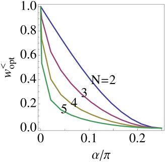
Figure 1: The lower bound $w_{\mathrm{opt}}^{<}$ on the local content $w_{\mathrm{opt}}$ in pure $N$-qubit generalized GHZ states as a function of $\alpha$ for $N=2,3,4,5$ (top to bottom).

III.3 General $N$-Qubit Case

Following the similar lines as above, we define $\theta_{0}$ by

$$\cos\theta_{0}\equiv-\frac{1-\tan^{\frac{2}{N}}\alpha}{1+\tan^{\frac{2}{N}}\alpha}\,,$$ (20)

at which $P_{Q}=0$ only when $\theta_{1}=\cdots=\theta_{N}=\theta_{0}$. We then suggest the following form of the local probability distribution $P_{L}$:

$$P_{L}=\frac{1}{2^{N}}\prod_{j=1}^{N}\left[1+r_{j}\operatorname{sgn}(\cos\theta_{j})\min\left(1,\left|\frac{\cos\theta_{j}}{\cos\theta_{0}}\right|\right)\right].$$ (21)

It is interesting to note that the resulting lower bound $w_{\mathrm{opt}}^{<}$ on the local content decreases rapidly with $N$. Its profile vs $\alpha$ for $N=2,3,4,5$ is shown in Fig. 1.

IV Upper Bound on the Local Content

So far we have focused on the lower bound $w_{\mathrm{opt}}^{<}(\rho)$ on the local content $w_{\mathrm{opt}}(\rho)$. Let us now briefly discuss the upper bound $w_{\mathrm{opt}}^{>}(\rho)$. As pointed out in Ref. Barrett , any Bell inequality can lead to an upper bound on $w_{\mathrm{opt}}(\rho)$. Following Refs. Barrett ; Scarani , suppose that a Bell inequality $P\leq P_{L}^{*}$ with a constant $P_{L}^{*}$ holds for all local probability distributions. Let $P_{NS}^{*}$ be the maximum value of $P$ under the condition of non-signaling condition. Then by Eq. (3) and the Bell inequality $P_{Q}^{*}(\rho)\leq w_{\mathrm{opt}}(\rho)P_{L}^{*}+[1-w_{\mathrm{opt}}(\rho)]P_{NS}^{*}$ where $P_{Q}^{*}$ is the quantum value of $P$ for the best choice of measurements. That is, the upper bound of the local content is given by

$$w_{\mathrm{opt}}^{>}=\frac{P_{NS}^{*}-P_{Q}^{*}}{P_{NS}^{*}-P_{L}^{*}}$$ (22)

An upper bound $w_{\mathrm{opt}}^{>}$ for $N=2$ was obtained based on this method in Ref. Scarani . Here we thus focus on the case of $N\geq 3$, where a Bell-type inequality was derived and shown to be violated maximally by GHZ states in Ref. Chenkai . One can show that $I_{L}^{*}=1$, $P_{NS}^{*}=2^{N-2}$, $P_{Q}^{*}=\sqrt{2^{N-2}\sin^{2}(2\alpha)+\cos^{2}(2\alpha)}.$ It immediately follows that

$$w_{\mathrm{opt}}^{>}=\frac{2^{N-2}-\sqrt{2^{N-2}\sin^{2}(2\alpha)+\cos^{2}(2\alpha)}}{2^{N-2}-1}.$$ (23)

Obviously, for product states ($\alpha=0$), the upper bound reaches 1, which is optimal. However, for the maximally entangled state ($\alpha=\pi/4$), the upper bound is not optimal, and approaches $1$ as $N\to\infty$ (to be compared with the result in the bipartite case, $N=2$, in Ref.Barrett ).

One can also consider the upper bound based on the Mermin-Ardehali-Belinskii- Klyshko (MABK) inequality MABK for the GHZ states (4). In this case, we find that the upper bound is $0$ for the maximally entangled state. However, for the generalized GHZ states such that $\sin(2\alpha)\leq 1/\sqrt{2^{N-1}}$, the upper bounds based on the MABK inequality are $1$ again. This is because such states do not violate MABK inequalities Scarani2 .

V Conclusion

In this paper, we have provided a decomposition for correlations in N-qubit generalized GHZ states into a nonlocal and fully local part. A general form of non-trivial local probability distribution $P_{L}$ of $N$ qubits has been proposed based on the properties of the convex decomposition of the quantum joint probability distribution into local and non-local parts, and thereby a lower bound on the local content in the GHZ states has been suggested. The improved local probability distribution in Scarani for pure two-qubit states turns out to be a special case of our results. Moreover, for a fixed value of $\alpha$, our lower bound on the local content decreases rapidly with $N$. We have also investigated the upper bound on the local content based on Bell-type inequalities.

- (1) J. S. Bell, Physics, 1, 195 (1964).
- (2) J. F. Clauser, M. A. Horne, A. Shimony and R. A. Holt, Phys. Rev. Lett. 26, 880 (1969).
- (3) A. Elitzur, S. Popescu, and D. Rohrlich, Phys. Lett. A 162, 25 (1992).
- (4) N. Brunner, N. Gisin, S. Popescu, and V. Scarani, Phys. Rev. A 78, 052111 (2008).
- (5) V. Scarani, Phys. Rev. A. 77, 042112 (2008).
- (6) J. Barrett, A. Kent, and S. Pironio, Phys. Rev. Lett. 97, 170409 (2006).
- (7) F. Zhang, J. Chen, C. Ren, and M. Shi, Phys. Lett. A. 374, 2429 (2009).
- (8) M. L. Almeida, D. Cavalcanti, V. Scarani, and A. Acin, Phys. Rev. A 81, 052111 (2010).
- (9) C. Branciard, N. Gisin, V. Scarani, Phys. Rev. A 81, 022103 (2010).
- (10) Given a choice of the quantization axes, let () be the azimuthal angle of the th qubit, in general, with . Then rotate the axes counterclockwise around axis by angle so that and hence .
- (11) K. Chen, S. Albeverio, S. M. Fei, Phys. Rev. A 74, 050101 (2006).
- (12) N. D. Mermin, Phys. Rev. Lett. 65, 1838 (1990); M. Ardehali, Phys. Rev. A 46, 5375 (1992); A.V. Belinskii and D. N. Klyshko, Phys. Usp. 36, 653 (1993).
- (13) V. Scarani and N. Gisin, J. Phys. A 34, 6043 (2001).