Abstract

Deformations of minimal surfaces lying in constant time slices in static space-times are studied. An exact and universal formula for a change of the area of a minimal surface under shifts of nearby point-like particles is found. It allows one to introduce a local temperature on the surface and represent variations of its area in a thermodynamical form by assuming that the entropy in the Planck units equals the quarter of the area. These results provide a strong support to a recent hypothesis that gravity has an entropic origin, the minimal surfaces being a sort of holographic screens. The gravitational entropy also acquires a definite physical meaning related to quantum entanglement of fundamental degrees of freedom across the screen.

1 Introduction

The fact that gravity is an emergent phenomenon dates back to ideas of the last century [1]. A renewal of the interest to this point of view in last years has been motivated by attempts to find a statistical explanation of the Bekenstein-Hawking entropy, see e.g. [2, 3, 4] and references therein. A possible source of the entropy are quantum correlations of underlying microscopical degrees of freedom across the black hole horizon [5, 6, 7].

By taking the black hole case as a guide a number of arguments have been presented in [8] that the entanglement entropy of fundamental degrees of freedom lying in a constant time slice and spatially separated by a surface $\cal B$ is

$$S({\cal B})={{\cal A}({\cal B})\over 4G}~{}~{}.$$ (1)

Here $G$ is the Newton coupling and $\cal A$ is the area of ${\cal B}$. Thus, (1) has the Bekenstein-Hawking form. Equation (1) holds in the semiclassical approximation if the low-energy limit of the fundamental theory is the Einstein gravity.

For realistic condensed matter systems the entanglement entropy associated to spatial separation of the system is a non-trivial function of microscopical parameters. Its calculation is technically involved and model dependent. The remarkable consequence of (1) is that the entanglement entropy in quantum gravity may not depend on a microscopical content of the theory, it is determined solely in terms of geometrical characteristics of the surface and low-energy gravity couplings.

Another feature established in [8] is related to the shape of the separating surface. Because $S({\cal B})$ includes contributions of all fundamental degrees of freedom quantum fluctuations of the geometry should be taken into account in a consistent way. For static space-times this requires that $\cal B$ is minimal surface, i.e. a surface with a least area. A relevant physical example of a minimal surface is the intersection of a constant time slice and the horizon of a stationary black hole. Thus, the Bekenstein-Hawking entropy can be considered as a particular case of the entanglement entropy (1).

The fact that $S({\cal B})$ is a macroscopic quantity which obeys certain dynamical laws points to similarity with a thermodynamical entropy. A natural question is whether the entanglement on the fundamental level admits a form of thermodynamical laws.

A first step in this direction was done in [8]. A calculation made there in the weak field approximation shows that a shift by a distance $l$ of a test particle with a mass $m$ out of the minimal surface results in the entropy change

$$\delta S({\cal B})=-\pi m~{}l~{}~{}.$$ (2)

A work needed to drag the particle by the background gravitational field is also proportional to $l$. Now by following the recent observation by Verlinde [9] one can relate the entropy change (2) and the work, the relation being an analog of the first law of thermodynamics. As we show this yields a local temperature on the surface. The temperature is proportional to the product of the acceleration of a static observer near the surface and the normal vector to $\cal B$.

A remarkable hypothesis of [9] is that gradients of the entropy of fundamental microscopical degrees of freedom in an underlying quantum gravity theory determine gradients of the gravitational field. To cut it short the force of gravity is an entropic force. The hypothesis is based on a number of assumptions for so called ‘holographic screens’ which store an information about fundamental microstates (’bits’) in such a way that a related entropy is proportional to the area of the screen. A variational formula for the entropy of the screen under the action of a point-like particle is postulated in the form like (2) and plays a key role in the arguments.

The main goal of this paper is to show that (2) follows from the properties of minimal surfaces in general static space-times and to establish an analogy between dynamics of minimal surfaces and thermodynamical systems. Minimal surfaces, therefore, may be considered as a sort of holographic screens with a well-understood dynamics. The form of this dynamics yields a strong support to the hypothesis of [9]. A possible relation of an entropic force and quantum entanglement has been discussed recently by a number of authors, see e.g. [10, 11], but not in the context of minimal surfaces.

In Section 2 we consider a weak field limit of gravity theory and study dynamics of minimal surfaces caused by shifts of test point-like particles located close to the surface. To make a connection with the ideas of [9] we start with a system which consists of two infinite non-intersecting planes and a massive source in between. The planes play the role of two components of a holographic screen. The Komar integral on the each plane equals half of the mass of the source. From this example we move to discussion of properties of a single minimal surface with the topology of a plane, introduce a local temperature on the surface and an analog of the first law.

The aim of next sections is to extend these results beyond the weak field approximation. In Section 3 we prove (2) for the entropy of a minimal surface in a slice in a static space-time which is a solution to the Einstein equations in a vacuum. The key property used here is an approximate isometry of the slice in the direction orthogonal to the surface.

Thermodynamical interpretation of the behavior of minimal surfaces in static space-times is discussed in Section 4. An advantage of taking holographic screens as minimal surfaces is in the clear physical meaning of the corresponding entropy. This opens a possibility to study further questions which we briefly describe.

We use units where $\hbar=c=k_{B}=1$.

2 Dynamics in a weak field approximation

Consider a gravitating source with the mass $M$. The geometry around the source is a static four-dimensional space-time $\cal M$. Constant-time slices in $\cal M$ are denoted by $\Sigma$. We need a holographic screen around the source which is a minimal surface in $\Sigma$. A closed minimal surface exists only around a black hole and it coincides with the black hole horizon. Therefore, we consider a screen which consists of two non-intersecting infinite components, ${\cal B}_{1}$, ${\cal B}_{2}$, with the source located in between. We assume that ${\cal B}_{k}$ are minimal surfaces in $\Sigma$ which have topology of a plane, see Fig. 1. The orientation of the surfaces can be specified by conditions at asymptotic infinity.

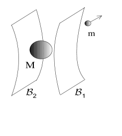
Figure 1: The figure shows two minimal surfaces, ${\cal B}_{1}$, ${\cal B}_{2}$, around a massive source with the mass $M$ and a test particle with the mass $m$. Shifts of the test particle result in a finite change of the area of the minimal surfaces.

It is convenient to start with the weak field approximation when the space-time metric is

$$ds^{2}=-\left(1+2\phi\right)dt^{2}+\left(1-2\phi\right)(dx^{2}+dy^{2}+dz^{2})~{}~{}~{}.$$ (3)

Here $\phi(r)=-{MG\over r}$, $r=\sqrt{x^{2}+y^{2}+z^{2}}$, is the gravitational potential of the source located at $r=0$. In the weak field approximation ${\cal B}_{k}$ are just parallel planes. One can direct the $z$ axis orthogonally to the surfaces and fix coordinates of the surfaces $z_{k}$. It is assumed that $|z_{k}|\gg MG$.

For the each surface one can define the following integral:

$${\cal E}({\cal B}_{k})={1\over 4\pi G}\int_{{\cal B}_{k}}d\sigma w_{n}~{}~{}~{},$$ (4)

where $d\sigma=dxdy$ and $w_{n}=\partial_{n}\phi$ is a normal component of the acceleration of a static observer located at the surface. The normal vectors to ${\cal B}_{k}$ are directed opposite to the source. The sum of the two integrals is the Komar mass which coincides with the mass of the source,

$${\cal E}={\cal E}({\cal B}_{1})+{\cal E}({\cal B}_{2})=M~{}~{}$$ (5)

because each ${\cal E}({\cal B}_{k})$ equals $M/2$. From this point of view the two-component screen is equivalent to a closed screen around the source.

Consider now the entropy (1) related to the surfaces. It is not difficult to see that the area of the surface in the weak field approximation is given by the integral

$${\cal A}({\cal B}_{k})=\int dxdy\left(1-2\phi(r_{k})\right)~{}~{}~{},$$ (6)

where $r_{k}=\sqrt{x^{2}+y^{2}+z_{k}^{2}}$. To avoid divergences in (6) one may assume that the surfaces have a large but finite size. Then according to (1)

$$S_{k}={{\cal A}({\cal B}_{k})\over 4G}=\bar{S}_{k}+\int d\textit{s}(r_{k})~{}~{}~{},$$ (7)

where $\bar{S}_{k}$ is a constant, an entropy associated to a plane, and

$$d\textit{s}(r)=-{1\over 2G}\phi(r)d\sigma~{}~{}.$$ (8)

By following [9] we define the number $dN$ of degrees of freedom on an element of the screen with the area $d\sigma$ as

$$d\textit{s}(r)=-{\phi(r)\over 2}dN~{}~{}$$ (9)

and come to equation

$$dN={d\sigma\over G}~{}~{}.$$ (10)

This coincides with the result by [9] but in our case (10) follows immediately from the the Bekenstein-Hawking relation (1). A relevance of (1) for the entropy on a holographic screen has been also pointed out in [12].

In this almost trivial setting one can study dynamics of minimal surfaces under the action of a test point-like particle. The gravitational field of the particle changes the shape of the surfaces. The area of the surface becomes

$${\cal A}({\cal B}_{k})=\int d\sigma\left[1-2\phi(r_{k})-2\phi^{\prime}(r^{\prime}_{k})\right]~{}~{}~{}.$$ (11)

Here $\phi^{\prime}(r^{\prime}_{k})=-mG/r^{\prime}_{k}$, $r^{\prime}_{k}=\sqrt{(x-x_{0})^{2}+(y-y_{0})^{2}+(z_{0}-z_{k})^{2}}$, is the gravitational potential of the particle on the surface, $m$ is the mass of the particle, and $x_{0},y_{0},z_{0}$ are its coordinates ($z_{0}>z_{k}$). A variation of the area of the surface under shifts of the particle is finite [8],

$$\delta{\cal A}({\cal B}_{k})=\delta z_{0}\int dxdy{2mG(z_{0}-z_{k})\over((x-x_{0})^{2}+(y-y_{0})^{2}+(z_{0}-z_{k})^{2})^{3/2}}=-4\pi mGl~{}~{}~{},$$ (12)

where $l=\delta z_{0}$ is the change of the distance between the particle and the surface. Displacements $\delta x_{0}$, $\delta y_{0}$ of the particle along the planes do not change the area because of a translational invariance. According to (20) the area of the surface increases if the particle moves towards the surface $(\delta z_{0}<0)$. The closer the particle to the surface the larger distortion of its shape.

If one restores all dimensional constants the variational formula for the entanglement entropy of the whole screen takes the form

$$\delta S=\delta S_{1}+\delta S_{2}=-2\pi{mc\over\hbar}l~{}~{}~{}.$$ (13)

It is assumed here that the particle moves out of the screen. In [9] the variational formula (13) has been postulated for surfaces of equal potentials.

Note that the situation is different when the particle moves between the surfaces. Then it is a part of the system and the Komar energy (5) is increased by the mass of the particle. Because the particle moves from one surface to the other variations $\delta S_{k}$ have opposite signs. Hence, when the particle moves staying inside the screen the whole entropy does not change, $\delta S=0$. There is an obvious analogy here between the two-component screen and a black hole horizon. The analogy can be strengthen if we recall that (1), as the entropy of entanglement, appears when the information about the states located inside the screen is not accessible for an outside observer.

We now return to the case when the particle is outside the screen. The gravitational field of a test particle moving in a vacuum changes a distribution of fundamental degrees of freedom and, therefore, affects the way they are entangled. On thermodynamical grounds a work $\delta W(x)$ which is required to change the state of underlying degrees of freedom on the holographic screen by dragging the test particle (located at a point with the coordinates $x$) is

$$\delta W(x)=-T(x)\delta S~{}~{}~{},$$ (14)

where $\delta S$ is the variation of the entropy (13) and $T(x)$ is a multiplier. One can then define an entropic force as force which performs the work (14)

$$\delta W(x)=-F(x)l~{}~{}~{}.$$ (15)

Here $F=-mw_{n}(x)$ is an external force and the work (15) is positive if the particle moves in the direction opposite to the gradient of the gravitational field. Expression for the multiplier follows from (13), (14),

$$T(x)={w_{n}(x)\over 2\pi}~{}~{}~{}.$$ (16)

By using analogy of (14) and the first law of thermodynamics $T(x)$ can be associated to a temperature, its expression being exactly the same as the result of [9]. Note that entropic force balances the component of force of gravity normal to the screen. Thus, in the Newtonian theory one may say that the gravity force has an entropic nature. The entropy increases in the direction of gradients of the gravitational potential.

For the following we need a definition of the temperature on the each surface. The components of the screen are equivalent, each carries the energy $M/2$, see (4), and acquires the same entropy variation, $\delta S_{k}=-\pi ml$. Therefore, the work required to change the state of the single component is just a half of the total work,

$$T_{k}(x)\delta S_{k}=-\frac{1}{2}\delta W(x)~{}~{}.$$ (17)

A local temperature on ${\cal B}_{k}$ can be defined in the limit when the test particle approaches the surface

$$T_{k}(x)=\left.{w_{n}(x)\over 2\pi}\right|_{x\in{\cal B}_{k}}~{}~{}~{}.$$ (18)

In the weak field approximation $T$ and $T_{k}$ coincide if the distance between the surfaces is much smaller than the distance of the test particle to the source.

Having this definition and the definition of the number of degrees of freedom on an element of the screen (12) we can rewrite the Komar integral (4) for a single surface as

$${\cal E}({\cal B}_{k})={1\over 2}\int_{{\cal B}_{k}}T_{k}dN~{}~{}.$$ (19)

The relation above looks as an ‘equipartition’ formula for an energy (see discussion in [13, 9]). This gives another justification of choosing a thermodynamic law for the single surface in the form (17). More arguments in favor of (17) follow in Section 4.

3 Dynamics in general background fields

Let us show that a minimal surface in a general static space-times allows the same variational formula (13) under the action of the gravitational field of a test particle.

We consider a static asymptotically flat space-time $\cal M$ with a metric $g_{\mu\nu}$ which is a solution to the Einstein equations. The dimensionality $n$ of $\cal M$ is not fixed. The space-time may describe either geometry around a black hole or a matter source located in a compact region. We are interested in constant time slices $\Sigma$ on $\cal M$ which are orthogonal to a time-like Killing vector field $\xi^{\mu}$. The metric on $\cal M$ can be written in the form

$$ds^{2}=-Bdt^{2}+dl^{2}=-B(x)dt^{2}+g_{ab}(x)dx^{a}dx^{b}~{}~{},$$ (20)

where components do not depend on time, $a,b$ are spatial indexes, and $dl^{2}$ is the metric on a slice $\Sigma$.

Let $\cal B$ be a minimal least area surface in $\Sigma$. The position of $\cal B$ is determined by a set of equations $X^{a}=X^{a}(y)$, where $y^{i}$ are coordinates on $\cal B$. The metric induced on $\cal B$ is $\gamma_{ij}=g_{ab}X^{a}_{,i}X^{b}_{,j}$. The position of $\cal B$ can be fixed by conditions at asymptotic infinity. If one places a test-particle near the surface the metric on $\cal M$ becomes $g_{\mu\nu}+h_{\mu\nu}$ and the area of the surface acquires a variation which we denote as ${\cal A}^{\prime}({\cal B})$. A trivial calculation shows that

$${\cal A}^{\prime}({\cal B})=\frac{1}{2}\int_{\cal B}\sqrt{\gamma}d^{n-2}y~{}\gamma^{ij}~{}X^{a}_{,i}X^{b}_{,j}h_{ab}~{}~{}.$$ (21)

The perturbations $h_{\mu\nu}$ can be considered in the linear order because the mass of the test particle is assumed to be small. The surface may also change its position but this causes no effect on ${\cal A}^{\prime}$ because the surface is minimal.

We allow a cosmological constant $\Lambda$ in the Einstein equations but assume that $\cal B$ does not intersect location of a gravitating source. By following the standard procedure one gets from the Einstein equations the equations for perturbations

$$L\bar{h}_{\mu}^{\nu}=16\pi G~{}t_{\mu}^{\nu}~{}~{},$$ (22)

$$L\bar{h}_{\mu}^{\nu}=-\nabla^{2}~{}\bar{h}_{\mu}^{\nu}-2R_{\mu\rho}~{}^{\nu\lambda}~{}\bar{h}^{\rho}_{\lambda}-{8\Lambda\over n-2}\bar{h}_{\mu}^{\nu}~{}~{},$$

where $R_{\mu\rho\nu\lambda}$ is the Riemann tensor of $\cal M$, and

$$\bar{h}_{\mu}^{\nu}=h_{\mu}^{\nu}-\frac{1}{2}h\delta_{\mu}^{\nu}~{}~{},$$ (23)

$h=h_{\mu}^{\mu}$. As usually, the gauge freedom has been used to set the condition $\nabla^{\lambda}\bar{h}_{\lambda\nu}=0$. The stress-energy tensor of the test particle which is at rest in coordinates (20) is

$$t^{\nu}_{\mu}=m\delta^{(n-1)}(x,x_{0})u^{\mu}u_{\nu}~{}~{}~{},$$ (24)

where $u^{\mu}=\xi^{\mu}/\sqrt{B}$ is the velocity and $m$ is the mass of the particle. The energy density measured by an observer with the velocity vector $u^{\mu}$ is $t_{\mu\nu}u^{\mu}u^{\nu}$. The energy density for static observers is $m\delta^{(n-1)}(x,x_{0})$. We choose the normalization

$$\delta^{(n-1)}(x,x^{\prime})=\delta^{(n-1)}(x-x^{\prime})/\sqrt{\det g_{ab}(x)}~{}~{},$$

$$\int_{\Sigma}t_{\mu\nu}u^{\mu}u^{\nu}\sqrt{\det g_{ab}}~{}d^{n-1}x=m~{}~{}~{}$$ (25)

to ensure that integration of this density over the slice $\Sigma$ yields the mass of the particle.

In (22) the wave operators on static solutions ($\partial_{t}\bar{h}_{\mu\nu}=0$) are reduced to covariant Laplacians on $\Sigma$ and a number of terms which depend on the acceleration $w^{\mu}=\nabla_{u}u^{\mu}$. For instance,

$$\nabla^{2}~{}\bar{h}_{0}^{0}=\Delta~{}\bar{h}_{0}^{0}-w^{a}\partial_{a}\bar{h}_{0}^{0}+2w^{2}~{}\bar{h}_{0}^{0}-2w_{a}w^{b}~{}\bar{h}_{b}^{a}~{}~{},$$ (26)

where $\Delta$ is a scalar Laplacian on $\Sigma$.

We consider the perturbations in a domain of the minimal surface $\cal B$ which is located in a vicinity of the particle. One expects that in this region the operator $L$ in (22) can be approximated by the covariant Laplacians $-\Delta$. This happens because spatial changes of the perturbations are so large that the curvature, $\Lambda$, and acceleration terms in $L$ can be neglected. In the coordinates (20) the only non-zero component of stress tensor (24) is $t^{0}_{0}$ and in the given approximation (22) yield the only non-vanishing perturbation

$$\bar{h}_{0}^{0}(x)=16\pi Gm~{}D(x,x_{0})~{}~{},$$ (27)

$$\Delta_{x}D(x,x^{\prime})=\delta^{(n-1)}(x,x^{\prime})~{}~{}.$$ (28)

This single perturbation, if one uses (23) and (21), results in the following variation of the area

$${\cal A}^{\prime}({\cal B})=-\frac{1}{2}\int_{\cal B}\sqrt{\gamma}d^{n-2}y~{}\bar{h}^{0}_{0}~{}~{}.$$ (29)

The approximation above does not mean that the slice $\Sigma$ is considered as a flat space and the minimal surface as a plane. Let us show that despite the fact that $\Delta$ is a curved Laplacian the dynamic of the minimal surface under the action of the particle is exactly the same as in the weak field approximation.

For further discussion it is convenient to use on $\Sigma$ the Gaussian normal coordinates which start on $\cal B$. The metric can be written as

$$dl^{2}=dz^{2}+\gamma_{ij}(z,y)dy^{i}dy^{j}~{}~{}.$$ (30)

The position of $\cal B$ is $z=0$ and $\gamma_{ij}(0,y)$ coincides with the metric on $\cal B$. The extrinsic curvature tensor for $\cal B$ in these coordinates is $k_{ij}(y)=-\frac{1}{2}\partial_{z}\gamma_{ij}(z,y)$. Because the surface is a minimal the trace $k_{ij}\gamma^{ij}(y)$ is vanishing, and the positivity of $\gamma^{ij}$ implies that

$$\partial_{z}\gamma_{ij}(0,y)=0~{}~{}.$$ (31)

It is important that (31) holds globally along the surface, i.e. there is a translational invariance along the $z$ direction in a narrow layer near $\cal B$. In this layer one can write

$$D(x,x^{\prime})=D(z-z^{\prime};y,y^{\prime})~{}~{},$$ (32)

$$D(z;y,y^{\prime})={1\over 2\pi}\int_{-\infty}^{\infty}dke^{ikz}\tilde{D}_{k}(y,y^{\prime})~{}~{},$$ (33)

where $\tilde{D}_{k}(y,y^{\prime})$ is an operator on $\cal B$ which is a solution to

$$(\tilde{\Delta}-k^{2})\tilde{D}_{k}(y,y^{\prime})=\delta^{(n-2)}(y,y^{\prime})~{}~{},$$ (34)

and $\tilde{\Delta}$ is a scalar Laplacian on $\cal B$.

Let $(z_{0},y_{0}^{i})$ be coordinates of the test particle on $\Sigma$, $z_{0}>0$. If the particle moves to a nearby point with coordinates $(z_{0}+l,y_{0}^{i}+l^{i})$ the area of the minimal surface changes as

$$\delta{\cal A}({\cal B})=\delta{\cal A}^{\prime}({\cal B})=\delta_{\parallel}{\cal A}^{\prime}({\cal B})+\delta_{\perp}{\cal A}^{\prime}({\cal B})~{}~{},$$ (35)

$$\delta_{\parallel}{\cal A}^{\prime}({\cal B})=-\kappa~{}l^{i}\int_{\cal B}\sqrt{\gamma}d^{n-2}y~{}{\partial\over\partial y_{0}^{i}}D(z-z_{0};y,y_{0})~{}~{},$$ (36)

$$\delta_{\perp}{\cal A}^{\prime}({\cal B})=-\kappa~{}l\int_{\cal B}\sqrt{\gamma}d^{n-2}y~{}{\partial\over\partial z_{0}}D(z-z_{0};y,y_{0})~{}~{},$$ (37)

where $\kappa=8\pi Gm$. Here we have used (27) and (29) and considered a linear order in coordinate shifts.

The variation is composed of two parts, $\delta_{\parallel}{\cal A}^{\prime}({\cal B})$, $\delta_{\perp}{\cal A}^{\prime}({\cal B})$, which correspond to shifts in directions parallel and normal to the surface. Let us consider first parallel variations. As in the previous section, we introduce an infrared regularization by assuming that $\cal B$ has a large but finite size. Then $\tilde{\Delta}$ on $\cal B$ has a discreet spectrum specified by some boundary conditions, the Drichlet or Neuman conditions, for example. Let $\varphi_{\lambda}(y)$ be a complete set of eigenmodes $\tilde{\Delta}\varphi_{\lambda}=\lambda\varphi_{\lambda}$, normalized as

$$\int_{\cal B}\sqrt{\gamma}d^{n-2}y~{}\varphi^{*}_{\lambda}(y)\varphi_{\lambda^{\prime}}(y)=\delta_{\lambda,\lambda^{\prime}}~{}~{}.$$ (38)

The solution to (34) can be written as

$$\tilde{D}_{k}(y,y^{\prime})=\sum_{\lambda}{\varphi_{\lambda}(y)\varphi^{*}_{\lambda}(y^{\prime})\over\lambda-k^{2}}~{}~{}~{}.$$ (39)

For the Neuman boundary conditions the operator $\tilde{\Delta}$ has a non-trivial constant eigenfunction which is a zero mode. For the Dirichlet conditions non-trivial constant modes are absent. Therefore, (38) can be used to write

$$\int_{\cal B}\sqrt{\gamma}d^{n-2}y~{}\varphi_{\lambda}(y)=c\delta_{\lambda,0}~{}~{},$$ (40)

where $c=\sqrt{\mbox{vol}({\cal B})}$ for Neuman conditions and $c=0$ for the Dirichlet conditions. One concludes that

$$\int_{\cal B}\sqrt{\gamma}d^{n-2}y~{}\partial_{y^{\prime}}\tilde{D}_{k}(y,y^{\prime})=0~{}~{}.$$ (41)

As a consequence of (33), (41) parallel shifts (36) do not change the area of the minimal surface, $\delta_{\parallel}{\cal A}^{\prime}({\cal B})=0$.

Let us turn to the normal part (37) of the variation. It can be written as a surface integral of the normal derivative,

$$\delta_{\perp}{\cal A}^{\prime}({\cal B})=\kappa~{}l\int_{\cal B}\sqrt{\gamma}d^{n-2}y~{}{\partial\over\partial z}D(z-z_{0};y,y_{0})~{}~{}.$$ (42)

When the infrared regularization is removed (42) can be converted into an integral of $\Delta D$ over $\Sigma$. After that one can use (28) to get for the area variation

$$\delta_{\perp}{\cal A}^{\prime}({\cal B})=-\frac{1}{2}\kappa~{}l=-4\pi mGl~{}~{}.$$ (43)

Note that the volume integral is equivalent to two surface terms, one on the surface $\cal B$ and another on a surface located at some coordinate $z>z_{0}$. The two surface terms for a point-like source are equivalent.

We conclude that variation of the area of a minimal surface is proportional to the change of the distance between the test particle and the surface, the form of the variation being exactly the same as in the weak field approximation. The area of the surface increases if the particle moves to the surface, $l<0$.

4 Discussion

As has been suggested in [9] gradients of the entropy of fundamental microscopical degrees of freedom in an underlying quantum gravity theory might determine the gradients of the gravitational field. Together with the fact that the gravitational field equations appear to follow from a maximization of the entropy [14, 9] one gets the strong evidence that gravity is an emergent phenomenon.

The results above are based on a number of postulates. In particular, one needs to clarify the physical meaning of the entropy. The key element in the reasonings of [9] are holographic screens which store an information, the total number of fundamental bits being proportional to the area of a screen. A remarkable fact that laws of gravity take the form of thermodynamical relations requires screens to be dynamical surfaces which change their shape under the action of the matter. Verlinde’s suggestion was to take the screens as equipotential surfaces. This is a straight way to relate entropy variations to gradients of the gravitational potential. However, it is not proved that dynamical properties of equipotential surfaces lead to the variational formula (13).

One of the avenues in looking for alternative dynamical screens is to study different kinds of horizons, as black hole mechanics teaches us. Some results [15] do indicate that, for example, trapping horizons allow an analog of the entropic force. The other option is to try to derive dynamical equations by studying lensing effects for a flow of trajectories passing through the screen. At the present moment, however, it is not clear which kind of trajectories has to be chosen, see [16] for some suggestions.

In previous sections we considered the screens as co-dimension 2 minimal surfaces in static space-times. In a quantum gravity theory a minimal surface encodes an information about entanglement of microscopical degrees of freedom spatially separated by this surface. The property that the entropy scales as the area of the surface is a physical fact which has been supported by computations in many-body systems [5, 6]. As for the minimal shape of the surface it is formed under quantum fluctuations of the geometry [8].

Not only the definite physical meaning of the entropy but also the possibility to derive explicit variational formula are among the important features of the minimal surfaces. Equations (35) and (43) result in formula (2) which yields the change of the entropy (1) under the shift of the test particle with respect to the screen by the distance $l$. Equation (2) does not depend on the form of background solution and dimensionality of space-time. It is the same relation as in the weak field approximation and further discussion of thermodynamical properties repeats arguments of Section 2.

Let us assume that $\Lambda=0$ and the test particle is suspended on a weightless rigid string near a minimal surface, the end of the string being in the region where the gravitational effects can be neglected. The surface is supposed to be between a massive source and the particle. Therefore, the acceleration vector of the particle $w^{\mu}$ is directed toward the surface. The force applied to the end of the string to hold the particle in a fixed position is $-m\sqrt{B}w^{\mu}$, see [17]. A distant observer can pull the end of the string to change position of the particle in the direction normal to the surface. The work done in this process is $\delta W(x)=m\sqrt{B}w_{n}(x)l$, where $w_{n}(x)=w^{\mu}(x)n_{\mu}(x)$ and $n_{\mu}$ is the unit vector normal to $\cal B$. The work is positive, if $l>0$, i.e. if the particle is shifted in the direction opposite to the acceleration, as it should be for a work done on the system by external forces. One can now relate the work and the variation of the entropy,

$$T(x)\delta S=-\frac{1}{2}\delta W(x)~{}~{}~{}.$$ (44)

The coefficient $T(x)$ has the meaning of a local temperature measured by a distant observer. With the help of (2) one finds

$$T(x)=\sqrt{B(x)}{w_{n}(x)\over 2\pi}~{}~{}~{}.$$ (45)

In (44) we took into account that the work should be distributed between two components of the holographic screen. In our case the second component is not considered. A single component with the topology of a hyperplane corresponds to half of the work because it carries half of the information about the entire system, see Section 2. This can be seen again from the fact that the ‘energy’ of the surface which is defined by the Komar integral

$${\cal E}({\cal B})={1\over 4\pi G}\int_{\cal B}\sqrt{B(x)}w_{n}(x)\sqrt{\gamma}d^{n-2}y={1\over 2}\int_{\cal B}TdN~{}~{}$$ (46)

equals half of the mass of the source.

As in (10), the quantity $dN=d\sigma/G$ is identified with the number of degrees of freedom per element of the screen with the area $d\sigma=\sqrt{\gamma}d^{n-2}y$. The ‘equipartition’ form of (46), see [13, 9], also supports the choice of the thermodynamical relation in the form (44).

It is instructive to discuss also the case when the massive source is a Schwarzschild black hole and the minimal surface goes near its horizon. There is a point where the distance between the surface and the horizon is minimal. At this point the normal vector to $\cal B$ is directed along the acceleration of a static observer. In the limit when the surface is shifted closer to the horizon the local temperature (45) tends to the Hawking temperature $T_{H}=\kappa/2\pi$ where $\kappa=\partial_{r}B(r_{H})/2$ is the surface gravity and the derivative is taken along the radial coordinate. This is another evidence for the validity of equations (44) and (45).

We see, therefore, that at least some variational formulas of minimal surfaces allow a thermodynamical analogy. It is a subject of further studies to find a deeper meaning behind this analogy. We also see that minimal surfaces considered as holographic screens provide a strong support to the hypothesis that gravity has an entropic origin [9].

Because the physical interpretation of the entropy associated to minimal surfaces is known one can pose problems for future research. We mention two of them. First, it is important to understand a possible role of quantum effects which may uncover the meaning of the local temperature (45), like quantum evaporation of black holes explains the meaning of the Hawing temperature.

Second, it is important to study generalization of equation (2) when the low energy limit of the gravity theory differers from the Einstein form. The simplest example of this situation are higher curvature corrections which may be present in the gravity action. The problem is that higher curvature terms change both formula (1) and equations which determine the shape of $\cal B$. If this generalization allows a thermodynamical analogy the ideas discussed here are robust.

References

- [1] A.D. Sakharov, Sov. Phys. Dokl. 12 (1968) 1040.
- [2] T. Jacobson, Black hole entropy and induced gravity, e-Print: gr-qc/9404039.
- [3] D.V. Fursaev, Phys. Part. Nucl. 36 (2005) 81, e-Print: gr-qc/0404038.
- [4] V.P. Frolov and D.V. Fursaev, Class. Quant. Grav. 15 (1998) 2041, e-Print: hep-th/9802010.
- [5] M. Srednicki, Phys. Rev. Lett. 71 (1993) 666, e-Print: hep-th/9303048.
- [6] L. Bombelli, R.K. Koul, J. Lee and R.D. Sorkin, Phys. Rev. D34 (1986) 373.
- [7] V. Frolov and I. Novikov, Phys. Rev. D48 (1993) 4545.
- [8] D.V. Fursaev, Phys. Rev. D77 (2008) 124002, e-Print: arXiv:0711.1221 [hep-th].
- [9] E. Verlinde, On the Origin of Gravity and the Laws of Newton, e-Print: arXiv:1001.0785 [hep-th].
- [10] Yun Soo Myung and Yong-Wan Kim, Phys. Rev. D81 (2010) 105012, e-Print: arXiv:1002.2292 [hep-th].
- [11] Jae-Weon Lee, Hyeong-Chan Kim and Jungjai Lee, Gravity as Quantum Entanglement Force, e-Print: arXiv:1002.4568 [hep-th].
- [12] V.V. Kiselev and S.A. Timofeev, The surface density of holographic entropy, e-Print: arXiv:1004.3418 [hep-th].
- [13] T. Padmanabhan, Mod. Phys. Lett. A25 (2010) 1129, e-Print: arXiv:0912.3165 [gr-qc].
- [14] T. Padmanabhan, Rept. Prog. Phys. 73 (2010) 046901, e-Print: arXiv:0911.5004 [gr-qc].
- [15] Rong-Gen Cai, Li-Ming Cao and Nobuyoshi Ohta, Phys. Rev. D81 (2010) 084012, e-Print: arXiv:1002.1136 [hep-th].
- [16] F. Piazza, Gauss-Codazzi Thermodynamics on the Timelike Screen, e-Print: arXiv:1005.5151 [gr-qc].
- [17] V.P. Frolov and I.D. Novikov, Black hole physics: Basic concepts and new developments, Dordrecht, Netherlands: Kluwer Academic (1998).