Scaling and synchronization in a ring of diffusively coupled nonlinear oscillators

Abstract

Chaos synchronization in a ring of diffusively coupled nonlinear oscillators driven by an external identical oscillator is studied. Based on numerical simulations we show that by introducing additional couplings at $(mN_{c}+1)$-th oscillators in the ring, where $m$ is an integer and $N_{c}$ is the maximum number of synchronized oscillators in the ring with a single coupling, the maximum number of oscillators that can be synchronized can be increased considerably beyond the limit restricted by size instability. We also demonstrate that there exists an exponential relation between the number of oscillators that can support stable synchronization in the ring with the external drive and the critical coupling strength $\varepsilon_{c}$ with a scaling exponent $\gamma$. The critical coupling strength is calculated by numerically estimating the synchronization error and is also confirmed from the conditional Lyapunov exponents (CLEs) of the coupled systems. We find that the same scaling relation exists for $m$ couplings between the drive and the ring. Further, we have examined the robustness of the synchronous states against Gaussian white noise and found that the synchronization error exhibits a power-law decay as a function of the noise intensity indicating the existence of both noise-enhanced and noise-induced synchronizations depending on the value of the coupling strength $\varepsilon$. In addition, we have found that $\varepsilon_{c}$ shows an exponential decay as a function of the number of additional couplings. These results are demonstrated using the paradigmatic models of Rössler and Lorenz oscillators.

I Introduction

Chaos synchronization has been receiving a great deal of interest for more than three decades Fujisaka and Yamada (1983a, b); Pecora and Corroll (1990); Pikovsky et al. (2001); Lakshmanan and Murali (1996). In particular, chaos synchronization in arrays of coupled nonlinear dynamical systems has been extensively investigated over the years in view of its diverse applications in spatially extended systems, neural process, networks, etc. Bohr and Christensen (1989); Heagy et al. (1994); Kocarev and Parlitz (1995); Francisco and Muruganandam (2003); Arenas et al. (2008); Osipov (1986). Linear arrays with periodic boundary condition (ring geometry) have been used widely in modeling physiological, biochemical and biological phenomena Osipov (1986); Matías et al. (1997); Matías and Güémez (1998). For example, morphogenesis in biological context Turing (1952) and transitions between different animal gaits have been explained by considering a model composed of a ring of coupled oscillators Collins and Stewart (1994). An important application of the ring geometry is that the resulting spatiotemporal patterns in the ensemble of coupled oscillators can be analyzed through symmetry arguments Collins and Stewart (1994); Matías et al. (1997). Recently several interesting dynamical properties/collective behaviors including amplitude death and chimera states have been identified in such a ring type configuration Osipov (1986); Matías et al. (1997); Matías and Güémez (1998); Reddy and Sen (2004); Abrams and Strogatz (2004); Deng and Huang (2002); Wang and Huang (2005, 2008); Jiang et al. (2003); Lorenzo et al. (1996); Harmov et al. (2006); Brandt et al. (2006).

Some of the recent studies have considered synchronization dynamics in both ring and linear arrays coupled together in order to understand the dynamics of basic units of networks Osipov (1986); Deng and Huang (2002); Wang and Huang (2005, 2008). Recently, interesting scaling behavior of correlation properties of interacting dynamical systems in such a configuration has been demonstrated Wang and Huang (2008). However, most of the studies have considered unidirectional coupling in both the ring and linear arrays. Because of the diverse nature of interaction in real world phenomena, we have considered diffusively (nearest-neighbor) coupled chaotic systems with ring geometry driven by an external identical drive in view of its widespread applications in engineering, robotics, networks, and physiological and biological systems Boccaletti et al. (2002); Rosenblum and Pikovsky (2004). For instance, cultured networks of heart cells are examples of biological structures with strong nearest-neighbor coupling Soen et al. (1999); Brandt et al. (2006).

The phenomenon of size instability, where a critical size of the number of oscillators upto which a stable synchronous chaotic state exists, of a uniform synchronous state in arrays of coupled oscillators with both periodic and free-end boundary conditions have been widely studied  Pecora and Corroll (1991); Pecora and Carroll (1998); Heagy et al. (1994); Matías and Güémez (1998); Matías et al. (1997); Bohr and Christensen (1989); Restrepo et al. (2004); Muruganandam et al. (1999a); Muruganandam (1999); Palaniyandi et al. (2005). Increasing the number of oscillators beyond this limit leads to desynchronization and the occurrence of spatially incoherent behavior (eg., high-dimensional or spatiotemporal chaos). The stability of synchronous chaos in coupled dynamical systems plays a crucial role in the study of pattern formation, spatiotemporal chaos, etc. Heagy et al. (1994); Muruganandam et al. (1999a); Restrepo et al. (2004); Muruganandam (1999); Rangarajan and Ding (2002); Chen et al. (2003). In this connection, using the paradigmatic models of Rössler and Lorenz oscillators we shall demonstrate in this paper that the maximal number of oscillators in the ring geometry that can support stable synchronous chaos can be increased by integer multiples of the original number of oscillators in the ring with additional couplings from the same drive oscillator. Furthermore, it is also found that the critical coupling strength and the number of oscillators which can be synchronized in the ring exhibit an exponential relation with a scaling exponent and indeed the relation remains unaltered even on increasing the number of couplings between the drive and the ring. In addition, the synchronization error displays a power law decay as a function of the noise intensity for a fixed value of the coupling strength indicating the existence of noise enhanced/induced synchronization. It is to be noted that small world networks can be generated by introducing additional couplings between randomly selected nodes to create shortest paths (links) between distant nodes Arenas et al. (2008). Further, recent studies on synchronizability of networks have been employing pinning control in which hubs in the networks are connected to the same drive node Arenas et al. (2008) as in our present study.

In particular, we consider here the Rössler and Lorenz oscillators in a ring geometry with diffusive coupling between them and driven by an external identical oscillator, whose strength is proportional to a parameter $\varepsilon$ (see Eq. (2) below). Based on numerical simulations, we find that the critical coupling strength, say $\varepsilon_{c}$, below which no synchronization exists $(\varepsilon<\varepsilon_{c})$, of the external drive increases exponentially with a scaling exponent, $\gamma\in(0.3,0.5)$, as a function of the number of oscillators in the array that supports a stable synchronous state. Further we observe that the number of oscillators which supports such a stable synchronous state can be increased in integer multiples by introducing additional couplings at the $(mN_{c}+1)$-th oscillator of the ring with same value of the coupling strength, where $m$ is the number of couplings and $N_{c}$ is the maximum number of oscillators in the ring that can sustain stable synchronization with a single coupling. Interestingly, this exponential relation is maintained while increasing the number of couplings, $m$, between the array and the external drive. In addition, we have found that $\varepsilon_{c}$ shows an exponential decay as a function of the number of additional couplings between the drive and the response array for a fixed number of oscillators in the array. Further, we find that these results are robust against Gaussian white noise of small intensity and the synchronization error exhibits a power law decay as a function of the noise intensity. These results also indicate the existence of both the phenomena of noise-enhanced and noise-induced synchronizations depending on the value of the coupling strength $\varepsilon$ beyond certain threshold values of the noise intensity. It is to be emphasized that all the numerical simulations throughout the manuscript have been repeated with several initial conditions and the results are the averages of a large number of realizations.

The structure of the paper is as follows. In Sec. II, we study synchronization in rings of diffusively coupled Rössler and Lorenz systems driven by external identical oscillators with a drive-response configuration. We show that in both the cases the critical coupling strength increases exponentially with the number of oscillators in the response array with a scaling exponent. In addition, the systems exhibit a power law decay of the synchronization error as a function of the noise intensity demonstrating noise-enhanced and noise-induced synchronizations depending on the value of the coupling strength. In Sec. III, we demonstrate that the size of the ring can be increased beyond the size instability limit by integer multiples of the maximum number of synchronized oscillators ($N_{c}$) in the ring with a single coupling for the same value of coupling strength. We also show that the same scaling relation with a characteristic exponent is valid for the case of arbitrary number of couplings also. Further, we examine the effect of noise on the robustness of the synchronous state for a fixed value of the noise intensity and as a function of the noise intensity for a fixed value of the coupling strength in all the cases. Finally, in Sec. IV, we present a summary and conclusions.

II Chaos synchronization in diffusively coupled oscillators driven by an external identical oscillator

For the present study, we consider a coupling scheme with drive-response configuration as shown in Fig. 1, in which the diffusively coupled circular array is driven by an external identical oscillator. Here ‘$0$’ denotes the external drive and ‘$1$’, ‘$2$’, …‘$N$’ denote the constituents of the response array with nearest neighbor (diffusive) coupling. For simplicity, we assume that all the oscillators in the drive-response configuration are identical. In this section, we study chaos synchronization in the response array when driven by the external drive. For this purpose, we have considered Rössler and Lorenz oscillators coupled

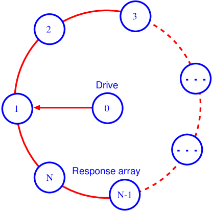
Figure 1: (color online) Schematic diagram of the ring of diffusively coupled oscillators driven by an external identical oscillator with drive-response configuration.

according to Fig. 1. The value of the diffusive coupling constant is chosen such that all the oscillators in the array are in a stable synchronous state. By varying the number of oscillators in the response array from $N=2$ onwards, we calculate the critical value of the coupling constant $\varepsilon_{c}$ at and above which the response array evolves in synchrony with the external drive.

II.1 Coupled Rössler system

First we analyse the coupled Rössler systems given by the dynamical equations

$$\dot{x}_{0}= \,-(y_{0}+z_{0}),$$

$$\dot{y}_{0}= \,x_{0}+ay_{0}$$

$$\dot{z}_{0}= \,b+z_{0}(x_{0}-c),$$ (1)

$$\dot{x}_{j}= \,-(y_{j}+z_{j})$$

$$\,+d(x_{j+1}+x_{j-1}-2x_{j})+\delta_{1,j}\varepsilon(x_{0}-x_{j}),$$ (2a)

$$\dot{y}_{j}= \,x_{j}+ay_{j}$$ (2b)

$$\dot{z}_{j}= \,b+z_{j}(x_{j}-c),\;\;j=1,2,\cdots,N,$$ (2c)

where $a=0.15$, $b=0.2$, $c=10$, $d=1$ and $\varepsilon$ is the coupling strength. Here the variable $x_{0}$, $y_{0}$ and $z_{0}$ correspond to the drive system and $x_{j}$, $y_{j}$ and $z_{j}$ $(j=1,2,\ldots,N)$ represent the diffusively coupled response array. The first oscillator of the response array (2) is driven by the drive (II.1). $\delta_{i,j}$ is the Kronecker delta function given by

$$\delta_{i,j}=\left\{\begin{array}[]{ll}1&\text{ for }i=j\\ 0&\text{ otherwise}.\end{array}\right.$$

The isolated system (II.1) exhibits chaotic behavior for the above choice of parameters with the Lyapunov exponents $\lambda_{1}\approx 0.1304>0$, $\lambda_{2}=0$ and $\lambda_{3}\approx-14.1405$.

Next we shall study the dynamics of the drive-response configuration (II.1) and (2). The value of the diffusive coupling constant $d$ is chosen such that it supports the maximum number of oscillators in the circular array to evolve in synchronous fashion. In the absence of any external coupling ($\epsilon=0$), the array of diffusively coupled Rössler systems (2) exhibits chaos synchronization in all the $N$ oscillators with $N\leq N_{\mbox{max}}$ with Heagy et al. (1994)

$$N_{\mbox{max}}=\frac{\pi}{\sin^{-1}\left(\sqrt{\lambda_{\mbox{max}}/4d}\right)},$$ (3)

where $\lambda_{\mbox{max}}$ is the maximal Lyapunov exponent. One can easily check that $N_{\mbox{max}}=17$ for the above choice of parameters.

As soon as the external drive is switched on ($\epsilon\neq 0$), the stable synchronous state of the diffusively coupled oscillators gets destroyed for small values of $\epsilon$. The number of oscillators in the response array (2) which retains synchronization with the drive (II.1) depends on the coupling strength $\epsilon$. To estimate the quality of synchronization, we define a measure, namely the synchronization error, as the Euclidean norm

$$\eta(t) =\frac{1}{N}\left\{\sum_{j=1}^{N}\left[(x_{0}-x_{j})^{2}+(y_{0}-y_{j})^{2}+(z_{0}-z_{j})^{2}\right]\right\}^{\displaystyle\frac{1}{2}},$$ (4)

In order to get a perfect synchronization in the drive-response configuration, (II.1) and (2), we require $\eta\to 0$ as $t\to\infty$. We remark here that all the simulations in the manuscript are performed for an average of over $100$ random initial conditions. By examining $\eta$, we extract the critical coupling strength $\varepsilon_{c}$ corresponding to the number of oscillators, $N$, in the response array, whose dynamics are entrained with that of the drive in phase space. For example, for $N=2$, we find the critical coupling strength as $\varepsilon_{c}=0.47$. The $\varepsilon_{c}$ values are given in Table 1 for different values of $N$. However, for $N\geq 6$, the system gets destabilized or becomes completely unstable, for any value of $\varepsilon\neq 0$.

Table 1: Critical coupling strength $\varepsilon_{c}$

Rössler system		Lorenz system
$N$	$\varepsilon_{c}$	$N$	$\varepsilon_{c}$
$2$	$0.447$	$2$	$12.528$
$3$	$0.721$	$3$	$20.288$
$4$	$1.134$	$4$	$31.334$
$5$	$1.882$	$5$	$51.486$

By careful examination of the numerical values, we realize that there is an exponential relation between the number of oscillators ($N$) in the response array that supports synchronization with the external drive and the critical coupling strength, $\epsilon_{c}$. By fitting the numerical values, one can easily establish the relation connecting $\epsilon_{c}$ and $N$ as

$$\varepsilon_{c}=\varepsilon_{0}\exp(\gamma N),$$ (5)

with the proportionality constant $\varepsilon_{0}=0.1665$ and the scaling exponent $\gamma=0.4842$.

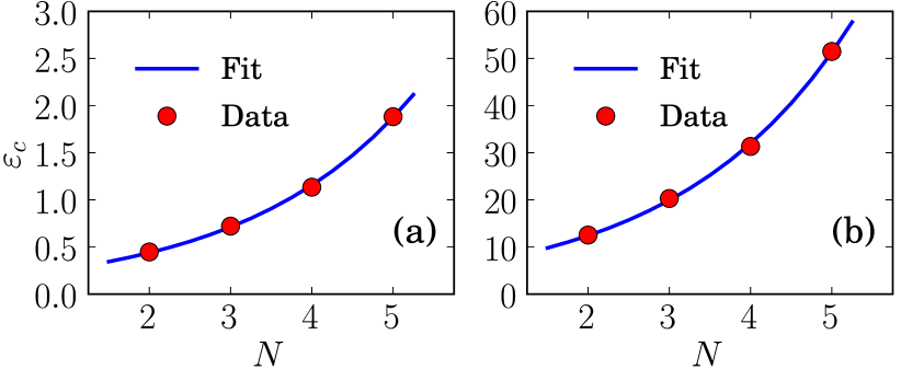
Figure 2: (color online) Variation of the critical coupling strength, $\varepsilon_{c}$, as a function of the number of oscillators, $N$, for (a) Rössler system ($\varepsilon_{0}=0.1665$ and $\gamma=0.4842$) and (b) Lorenz system ($\varepsilon_{0}=4.8158$ and $\gamma=0.4731$). Filled circles correspond to the numerical data and solid lines are the plot of $\varepsilon_{c}$ using relation (5).

The critical coupling strength as a function of the number of oscillators is shown in Fig. 2(a), where the filled circles correspond to numerical data and the solid line is the fitted data using the relation (5).

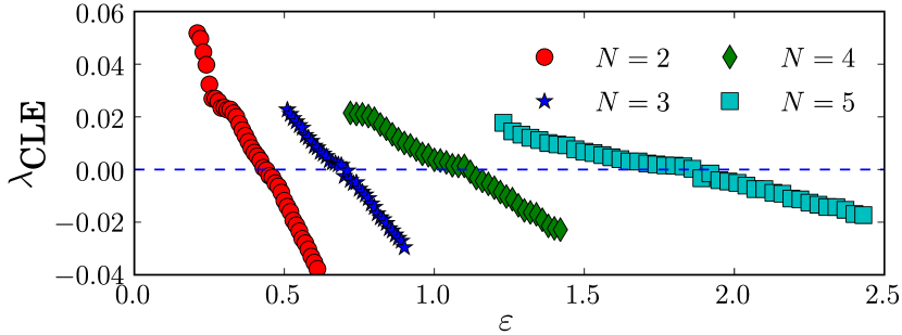
Figure 3: (color online) Conditional Lyapunov exponents of the coupled Rössler system (2) for different values of the number of oscillators ($N$) in the array as a function of the coupling strength.

The above result is also confirmed by calculating the conditional Lyapunov exponents (CLEs) of the response array by increasing the number of the coupled oscillators $N$. Here by CLE we mean the largest Lyapunov exponent of the response array, which of course should be less than zero in order to have a synchronous state. Fig. 3 shows the variation of CLEs as a function of $\varepsilon$ for the various numbers of oscillators in the response array. From Fig. 3, one can identify that the value of $\varepsilon_{c}$ for each $N$, where a transition of the CLE from positive to negative value occurs, agrees with the value of $\varepsilon_{c}$ given in Table I.

II.2 Coupled Lorenz systems

Next we consider the case of the Lorenz system described by the following set of equations Sparrow (1982); Lorenz (1963) as the drive,

$$\dot{x}_{0}= \,\sigma(y_{0}-x_{0}),$$

$$\dot{y}_{0}= \,rx_{0}-y_{0}-x_{0}z_{0}$$

$$\dot{z}_{0}= \,-\beta z_{0}+x_{0}y_{0},$$ (6)

where $\sigma=10$, $r=23$ and $\beta=1$. A ring of diffusively coupled Lorenz systems for the response array can be represented by the following set of coupled equations,

$$\dot{x}_{j}= \,\sigma(y_{j}-x_{j})+d(x_{j+1}+x_{j-1}-2x_{j})$$

$$\,\qquad\qquad\qquad+\delta_{1,j}\varepsilon(x_{0}-x_{j}),$$ (7a)

$$\dot{y}_{j}= \,rx_{j}-y_{j}-x_{j}z_{j}$$ (7b)

$$\dot{z}_{j}= \,-\beta z_{j}+x_{j}y_{j},\;\;j=1,2,\cdots,N,$$ (7c)

where $d$ is the diffusive coupling constant and $\varepsilon$ is the coupling strength of the external drive. One may note that the isolated system (6) exhibits chaotic behavior for the above choice of parameters with the Lyapunov exponents $\lambda_{1}=0.6075>0$, $\lambda_{3}=0$ and $\lambda_{3}=-17.9194$.

We study the variation of the critical coupling strength as a function of the number of oscillators in the response array by numerically examining the synchronization error $\eta$ in a similar fashion as in the case of the coupled Rössler oscillators. For this purpose, we fix the diffusive coupling constant as $d=30$. In this case, the response array (7), in the absence of external drive $(\varepsilon=0)$, supports a maximum of $N=9$ oscillators in the stable synchronous state as per Eq. (3).

When the external coupling is switched on, the synchronization in the array (7) gets lost. However, by choosing the number of oscillators, $N$, and the coupling strength, $\varepsilon$, appropriately one can synchronize the array with the external drive. The values of $\varepsilon_{c}$ for different numbers of oscillators in the response

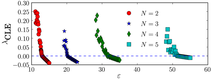
Figure 4: (color online) Conditional Lyapunov exponents of the coupled Lorenz system (7) for different values of the number of oscillators in the array as a function of the coupling strength.

array, $N$, are also given in Table 1. Fig. 2(b) depicts the plot of $N$ versus $\varepsilon_{c}$. It is easy to see that, as in the case of the coupled Rössler oscillators discussed above, $\varepsilon_{c}$ again increases exponentially as a function of $N$ according to the relation (5) with $\varepsilon_{0}=4.8158$ and $\gamma=0.4731$.

The above results have also been examined by calculating the conditional Lyapunov exponents associated with (7) and it is confirmed that the largest CLE (cf. Fig. 4) transits from positive to negative value at the critical coupling strength of a given $N$ as shown in Table 1.

So far, we have considered Rössler and Lorenz oscillators with a ring geometry and driven by an external identical oscillator in a drive-response configuration. Based on numerical simulations, we have found that there is an exponential relation connecting the critical value of the coupling strength $\varepsilon_{c}$ and the number of oscillators in the response array $N$ that evolve in synchrony with the external drive with a scaling exponent $\gamma\approx 0.48$ for both the Rössler and Lorenz oscillators. Next, we will examine the effect of Gaussian white noise on the stability of synchronization of the coupled oscillators.

II.3 Effect of noise

We have examined the robustness of the synchronous states of the coupled oscillators by including Gaussian white noise to the first variable of all the systems. Interestingly, we find that the results obtained remain unaltered

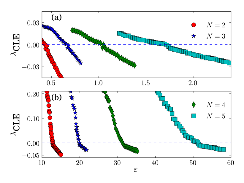
Figure 5: (color online) Conditional Lyapunov exponents of the coupled (a) Rössler and, (b) Lorenz systems for different values of the number of oscillators in the array as a function of the coupling strength in the presence of Gaussian white noise with intensity $D_{0}=0.001$.

for small values of the noise intensity and the synchronization error, $\eta$, follows a power law decay as the intensity of the noise is increased resulting in noise-enhanced and noise-induced synchronizations depending on the value of the coupling strength. It is of interest to note that similar noise-enhanced phase synchronization in two coupled noisy Rössler oscillators Osipov (1986); Zhou et al. (2002) and noise-induced phase synchronization in two coupled Rössler and Lorenz oscillators Osipov (1986); Zhou et al. (2002) have been observed.

In particular, we have included the Gaussian white noise, $\sqrt{2aD_{0}}\xi(t)$ with $a=0.01$ to the $x$ variable of all the coupled systems including the drive after every time step, where $D_{0}$ is the noise intensity and $\xi(t)$ is the Gaussian white noise. We have calculated the CLEs for both the Rössler and Lorenz oscillators as in the previous section by including a small noise with noise intensity $D_{0}=0.001$, which are plotted in Figs. 5(a) and  5(b), respectively. It is evident from this figure that the critical values of $\varepsilon$ for the chosen value of the noise intensity remain almost the same as in Figs. 3 and  4 for the Rössler and Lorenz oscillators, respectively. Hence, the exponential relation between the number of oscillators in the ring and their corresponding $\varepsilon_{c}$ remains the same in the presence of small noise also.

Furthermore, we have calculated the synchronization error $\eta$ by increasing the noise intensity $D_{0}$ at the threshold value of $\varepsilon$, namely $\varepsilon_{c}$, shown in Table 1. The average synchronization error $\langle\eta\rangle$, where $\langle\cdot\rangle$ denotes the time average over $500\,000$ time steps, for different values of $N$ in the ring as a function of noise intensity $D_{0}$ is shown in Figs. 6(a) and  6(b) for the Rössler and Lorenz systems, respectively.

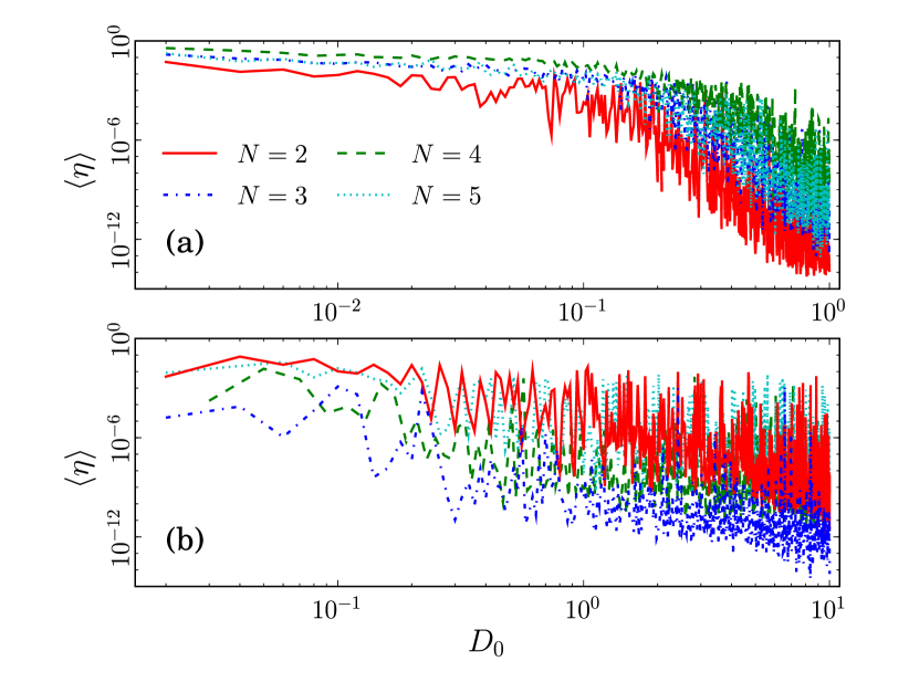
Figure 6: (color online) Time averaged synchronization error $\langle\eta\rangle$ for different numbers of oscillators in the ring as a function of the noise intensity $D_{0}$ for a fixed value of $\varepsilon_{c}$ displaying a power law decay for (a) the Rössler oscillators in the range $D_{0}\in(0.01,1)$, and (b) the Lorenz oscillators in the range $D_{0}\in(0.01,10)$.

The average synchronization error for both the Rössler and Lorenz systems for different numbers of oscillators in the ring follows a power law decay as a function of the noise intensity $D_{0}$ beyond certain threshold values of $D_{0}$, i.e, $D_{0}\geq 0.01$.

In our studies, we have fixed the value of the coupling strength $\varepsilon$ at the critical coupling strength $\varepsilon_{c}$ as shown in Tables for different values of $N$. On increasing the noise intensity $D_{0}$, the synchronization error follows a power-law decay as a function of $D_{0}$ after certain threshold value of noise intensity. This naturally corresponds to a noise-enhanced synchronization and also confirms the robustness of the synchronous state. Interestingly, we have also observed that by fixing $\varepsilon$ at a value less than that of the synchronization threshold $\varepsilon_{c}$, noise can induce synchronization between the ring and the drive oscillator. The synchronization error again shows a power-law decay as a function of the noise intensity (exactly similar to Figs. 6 omitted here to avoid repetition), exhibiting noise-induced synchronization. Thus we have observed both the phenomena of noise-enhanced and noise-induced synchronizations depending upon the choice of $\varepsilon$.

III Overcoming size instability by introducing additional couplings

In the above, we have pointed out that, when one considers an array of diffusively coupled chaotic oscillators (with a ring geometry) driven by an external identical forcing in the drive-response configuration, the critical coupling strength of the external drive required to synchronize the response array varies exponentially with the number of oscillators within the synchronization regime. As a consequence of the exponential relation, the number of oscillators in the response array that can be synchronized with the external drive is limited to $4$ or $5$ because one requires a high coupling strength, which results in desynchronization above a certain threshold value of the coupling strength due to size instability. However, we wish to point out here that it is possible to increase the number of oscillators in the response array, which are synchronized with the external drive by increasing the number of couplings. In Fig. 7 we show a schematic diagram

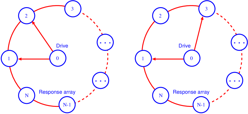
Figure 7: (color online) Schematic diagram of the ring of diffusively coupled oscillators driven by an external identical oscillator with additional coupling in (a) first neighbor and (b) second neighbor.

for the realization of the drive-response configuration with more than one coupling. In this section we explore the possibility of increasing the number of oscillators that evolve in synchrony with the drive and the robustness of the scaling exponent $\gamma$ when one introduces more number of couplings between the drive and the response array.

In order to study the effect of making more number of couplings between the drive and the response array, we again consider the coupled Rössler systems as discussed earlier in Sec. II.1. The drive system is assumed to follow the same set of equations (II.1) as before. Then the governing equations for the response array can be written as

$$\dot{x}_{j}= \,-(y_{j}+z_{j})$$

$$\,+d(x_{j+1}+x_{j-1}-2x_{j})+p_{j}(x_{0}-x_{j}),$$ (8a)

$$\dot{y}_{j}= \,x_{j}+ay_{j},$$ (8b)

$$\dot{z}_{j}= \,b+z_{j}(x_{j}-c),\;\;j=1,2,\cdots,N,$$ (8c)

where

$$p_{j}=\varepsilon\sum_{k=0}^{m-1}\delta_{j,kl+1},\;\;\;\;\delta_{j,kl+1}=\left\{\begin{array}[]{l}1\;\;\text{for}\;\;j=kl+1,\\ 0\;\;\text{otherwise}.\end{array}\right.$$ (11)

and $\varepsilon$ corresponds to the coupling strength. Here $m$ denotes the number of couplings and $l$ represents the $l$-th neighbor of the first oscillator in the response array. For example, $l=1$ for the first neighbor, $l=2$ for the second neighbor and so on.

III.1 Second coupling at the first neighbor

First let us consider the case in which there is a second coupling (of the same strength as the first one) between the external drive and the response array in the immediate neighborhood of the first oscillator, that is, $l=1$ in Eq. (11), which is already coupled to the drive [cf. Fig. 7(a)]. For simplicity, we consider the coupled Rössler systems (II.1) and (8) with $N=3$ with coupling at the first and second oscillators in the array. Now, interestingly it is easy to see that the critical coupling strength required to synchronize all the three oscillators in the array gets reduced to $\varepsilon_{c}\approx 0.311$ from $\varepsilon_{c}\approx 0.407$ (see Table 1). Similarly, up to $N=6$ the second additional coupling helps to reduce the critical values of $\varepsilon$ as tabulated in Table 2 for the

Table 2: Critical coupling strength $\varepsilon_{c}$ for second coupling at the first neighbour

Rössler system		Lorenz system
$N$	$\varepsilon_{c}$	$N$	$\varepsilon_{c}$
$3$	$0.311$	$3$	$9.189$
$4$	$0.441$	$4$	$12.895$
$5$	$0.647$	$5$	$18.435$
$6$	$1.056$	$6$	$28.297$

coupled Rössler oscillators. The same analysis can be extended to the Lorenz oscillators (6)-(7) as well. Again the results are tabulated in Table 2. It may be noted that for such a second additional coupling one additional oscillator, namely $N=6$, in the ring can be synchronized compared to the case of a single coupling (see Table 1). Further, the critical values of $\varepsilon$ in Table 2 again show an exponential relation with the number of synchronized oscillators in the array as shown in

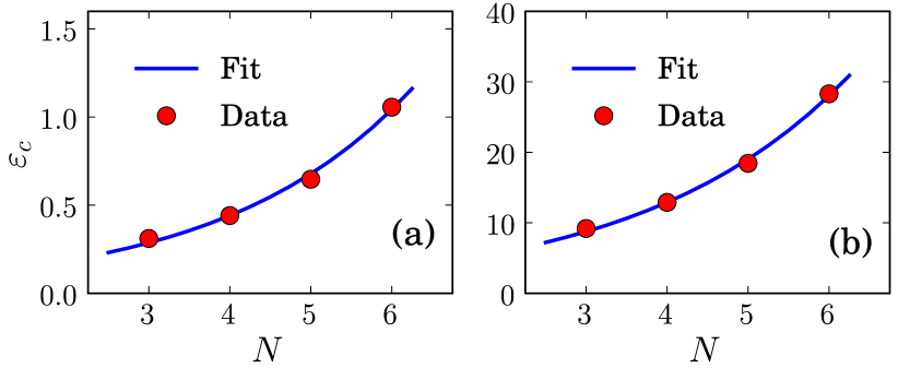
Figure 8: (color online) The variation of the critical coupling strength, $\varepsilon_{c}$, as a function of the number of oscillators, $N$, for second additional coupling at the first neighbor of the first coupling for (a) Rössler system ($\varepsilon_{0}=0.0788$ and $\gamma=0.43303$) and (b) Lorenz system ($\varepsilon_{0}=2.7351$ and $\gamma=0.3878$). Filled circles corresponds to the numerical data and solid lines are the plot of $\varepsilon_{c}$ using relation (5).

Figs. 8(a) and  8(b) for the Rössler and Lorenz oscillators, respectively. Here the proportionality constant $\varepsilon_{0}=0.0788$ and the scaling exponent $\gamma=0.4303$ for the Rössler oscillators and $\varepsilon_{0}=2.7351$ and $\gamma=0.3878$ for the Lorenz oscillators.

The conditional Lyapunov exponents of the coupled Rössler and Lorenz oscillators for $N=3,4,5$ and $6$ oscillators in the ring as a function of $\varepsilon$ is shown in Figs. 9(a) and 9(b), respectively. It is to be noted that all the CLEs change their values from positive to negative near the critical values of $\varepsilon$ as in Table 2.

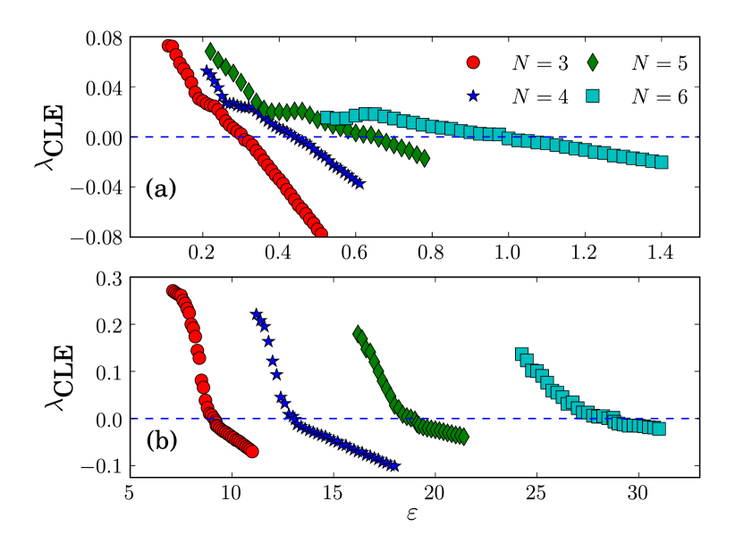
Figure 9: (color online) Conditional Lyapunov exponents of the (a) Rössler and, (b) Lorenz systems for different values of the numbers of oscillators ($N$) in the array as a function of the coupling strength with the second additional coupling at the first neighbor of the first coupling.

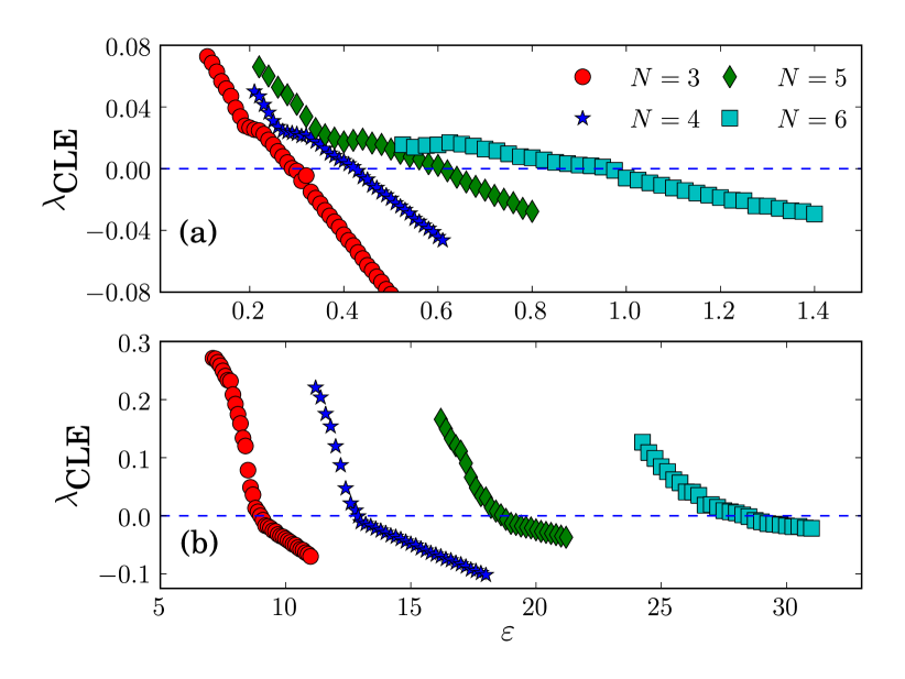
Figure 10: (color online) Conditional Lyapunov exponents of the (a) Rössler and, (b) Lorenz systems for different values of the number of oscillators ($N$) in the array as a function of the coupling strength with the second additional coupling at the first neighbor of the first coupling in the presence of Gaussian white noise with intensity $D_{0}=0.001$.

We have also investigated the effect of noise in the present case as well. The CLEs of both the coupled Rössler and Lorenz oscillators for different $N$ values in the ring for the noise intensity $D_{0}=0.001$ is plotted in Figs. 10(a) and 10(b) as a function of $\varepsilon$. Again the CLEs change their signs almost at the same critical values of $\varepsilon$ as the CLEs of the coupled oscillators without noise [Figs. 9(a) and 9(b)] thereby preserving the same exponential relation between the critical values of $\varepsilon$ and the number of oscillators synchronized in the ring. Further,

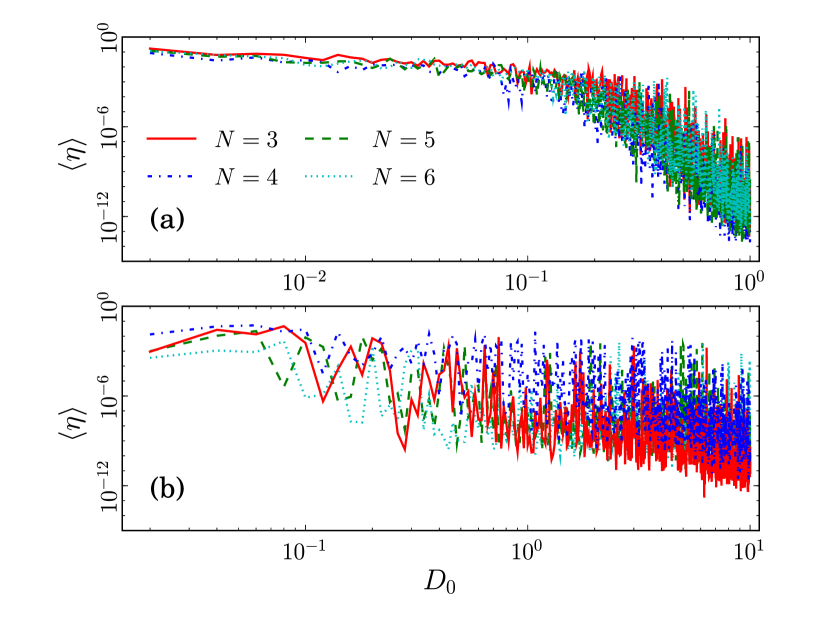
Figure 11: (color online) Time averaged synchronization error $\langle\eta\rangle$ for different number of oscillators in the ring as a function of noise intensity $D_{0}$ for fixed value of $\varepsilon_{c}$ displaying a power-law decay (a) the Rössler oscillators in the range $D_{0}\in(0.01,1)$, and the Lorenz oscillators in the range $D_{0}\in(0.01,10)$ with the second additional coupling at the first neighbor of the first coupling.

the synchronization error $\langle\eta\rangle$ follows a power law decay as a function of the noise intensity $D_{0}$ for both the Rössler and Lorenz oscillators as shown in Figs. 11(a) and 11(b) beyond certain threshold values of $D_{0}$ for a fixed value of $\varepsilon_{c}$ given in Table 2 illustrating noise-enhanced synchronization. Further, a similar relation can be obtained between $\langle\eta\rangle$ and $D_{0}$ for values of $\varepsilon<\varepsilon_{c}$ confirming the existence of noise-induced synchronizations.

III.2 Second coupling at the second neighbor

Next, by introducing a second coupling at the second neighbor (instead of the first one), $l=2$, of the first coupling, we find that one can synchronize two additional oscillators in the ring compared to the number of synchronized oscillators with a single coupling. Likewise, introducing the second coupling at the third neighbor [cf. Fig. 7(b)] of the first oscillator $(l=3)$ in the

Table 3: Critical coupling strength $\varepsilon_{c}$ for second coupling at the second neighbour.

Rössler system		Lorenz system
$N$	$\varepsilon_{c}$	$N$	$\varepsilon_{c}$
$4$	$0.405$	$4$	$12.212$
$5$	$0.563$	$5$	$16.231$
$6$	$0.814$	$6$	$21.883$
$7$	$1.156$	$7$	$31.987$

array results in increasing the number of oscillators that are synchronized with the drive by $3$. Similarly, introducing the second coupling at the $N$-th neighbor will increase the synchronized oscillators in the ring by $N$. Thus from the Table 1 for single coupling, we can realize that it is possible to synchronize up to $10$ oscillators (instead of $5$) with the introduction of a second coupling at reduced critical coupling strength.

The critical values of the coupling strength $\varepsilon_{c}$ and their corresponding number of synchronized oscillators in the ring for both the Rössler and Lorenz oscillators for the second coupling at the second neighbor are tabulated in Table 3, which again displays an exponential relation as shown in Figs. 12(a) and 12(b).

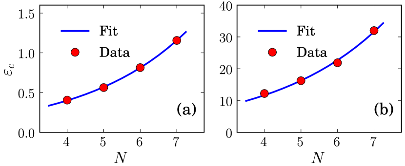
Figure 12: (color online) The variation of the critical coupling strength, $\varepsilon_{c}$, as a function of the number of oscillators, $N$, for second additional coupling at the second neighbor of the first coupling for (a) Rössler system ($\varepsilon_{0}=0.0972$ and $\gamma=0.3536$) and (b) Lorenz system ($\varepsilon_{0}=3.0908$ and $\gamma=0.3321$). Filled circles corresponds to the numerical data and solid lines are the plot of $\varepsilon_{c}$ using relation (5).

The proportionality constant is estimated as $\varepsilon_{0}=0.0972$ and the scaling exponent $\gamma=0.3536$ for the Rössler oscillators and $\varepsilon_{0}=3.0908$ and $\gamma=0.3321$ for the Lorenz oscillators. These critical values of $\varepsilon$ are also confirmed by the transitions in the value of the CLEs of the coupled Rössler and Lorenz oscillators as shown in Figs. 13(a) and 13(b).

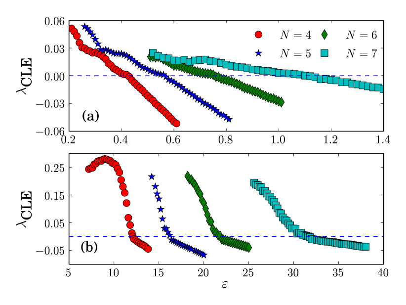
Figure 13: (color online) Conditional Lyapunov exponents of the (a) Rössler and, (b) Lorenz systems for different values of the number of oscillators in the array as a function of the coupling strength with the second additional coupling at the second neighbor of the first coupling.

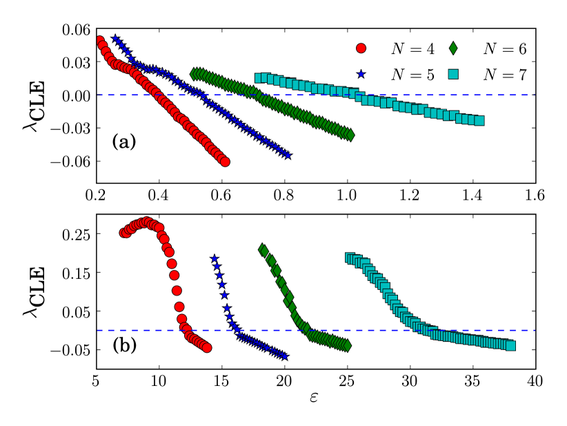
Figure 14: (color online) Conditional Lyapunov exponents of the (a) Rössler and, (b) Lorenz systems for different values of the number of oscillators in the array as a function of the coupling strength with the second additional coupling at the second neighbor of the first coupling in the presence of the Gaussian white noise with noise intensity $D_{0}=0.001$.

The conditional Lyapunov exponents of both the oscillators as a function of $\varepsilon$ with the noise intensity $D_{0}=0.001$ for $N=4,5,6$ and $7$ oscillators in the ring are shown in Figs. 14(a) and 14(b). It is evident from this figure that the critical value of $\varepsilon$ for small noise intensity is almost the same as that of the oscillators without noise [cf. Figs. 13(a) and 13(b)], indicating the robustness of the synchronous state and the exponential relation (5) with the addition of small noise. Further the

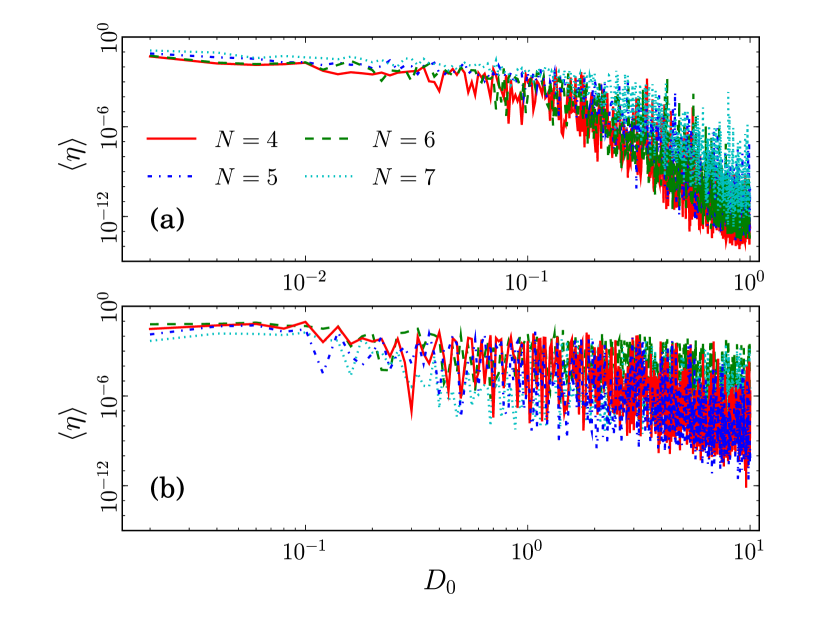
Figure 15: (color online) Time averaged synchronization error $\langle\eta\rangle$ for different number of oscillators in the ring as a function of noise intensity $D_{0}$ for fixed value of $\varepsilon_{c}$ displaying power-law decay for (a) the Rössler oscillators in the range $D_{0}\in(0.01,1)$, and (b) the Lorenz oscillators in the range $D_{0}\in(0.01,10)$ with the second additional coupling at the second neighbor of the first coupling.

power law decay of the synchronization error as a function of the noise intensity [Figs. 15(a)-(b)] beyond certain threshold values of $D_{0}$ for the value of $\varepsilon_{c}$ for both the oscillators confirming the existence of noise-enhanced synchronization. Exactly similar figures can be obtained by fixing the coupling strength to be less than $\varepsilon_{c}$ indicating the existence of noise-induced synchronization.

III.3 Couplings at the $N$-th neighbors

Let $N_{c}$ be the maximum number of oscillators in the response array that are synchronized with the external drive for a given $\varepsilon_{c}$ for $m=1$. Then, by introducing a second coupling, $(m=2)$ in eq. (11), at $N_{c}+1$ one can synchronize up to a maximum of $2N_{c}$ oscillators in the response array with the external drive for the same coupling strength $\varepsilon_{c}$. One can also introduce a third coupling in the response array, $(m=3)$ in eq. (11), in the same fashion in which the second coupling is introduced where one can synchronize a maximum $3N_{c}$ oscillators in the response array. In this way one can increase the number of oscillators (size) in the response array that evolve in synchrony with the external drive to $mN_{c}$ by introducing $m$ couplings at the oscillator index $1$, $N_{c}+1$, $2N_{c}+1$, …, $(m-1)N_{c}+1$, respectively, with the same critical coupling $\varepsilon_{c}$.

In the following we shall illustrate this result using the second and third couplings at the oscillators with the indices $N_{c}+1$ and $2N_{c}+1$, respectively. It is known from Section II that the maximum number of oscillators that can be synchronized with the drive with a single coupling is $N_{c}=5$. The CLEs of the Rössler and Lorenz oscillators with the second coupling, $(m=2)$, at the oscillator in the ring with the index $N_{c}+1=6$ and the third coupling, $(m=3)$, at the oscillator index $2N_{c}+1=11$ along with the CLE of the $N_{c}$ oscillators in the ring with a single

Figure 16: (color online) Conditional Lyapunov exponents of the (a) Rössler and, (b) Lorenz system for different values of the number of oscillators in the array as a function of the coupling strength with the second and the third additional couplings at the $N$-th and $2N$-th neighbor, respectively, of the first coupling.

coupling are shown in Figs. 16(a) and 16(b) as a function of $\varepsilon$. It clearly shows that the $mN_{c}$ oscillators in the ring with couplings at $m=1,2$ and $3$ are synchronized exactly at the same critical value of the coupling strength $\varepsilon_{c}$. Hence, it is evident that the number of synchronized oscillators can be increased beyond the size instability to any desired amount by introducing additional couplings at the $(mN_{c}+1)$-th oscillators for the same value of $\varepsilon_{c}$.

We have also examined the effect of noise as in the previous cases. The CLEs of the Rössler and Lorenz oscillators with the second and the third couplings at the oscillators with the indices $N_{c}+1$ and $2N_{c}+1$ with the noise intensity $D_{0}=0.001$ for fixed value of $\varepsilon_{c}$ are shown in Figs. 17(a) and 16(b), respectively. The synchronization

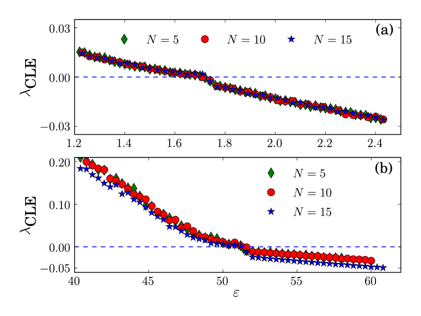
Figure 17: (color online) Conditional Lyapunov exponents of the (a) Rössler and, (b) Lorenz system for different values of the number of oscillators in the array as a function of the coupling strength with second additional coupling at the $N$-th and $2N$-th neighbors, respectively, of the first coupling in the presence of Gaussian white noise with intensity $D_{0}=0.001$.

error also displays a power law decay as a function of the noise intensity $D_{0}$ as shown in Figs. 19(a) and 19(b) beyond after certain threshold values of $D_{0}$ for both the coupled Rössler and Lorenz oscillators confirming the robustness of the synchronous states and the noise-enhanced synchronization. Further these systems of coupled oscillators also display noise-induced synchronization by exhibiting similar figures as a function of $D_{0}$ for $\varepsilon$ less than $\varepsilon_{c}$.

III.4 Effect of additional couplings

In addition to the effect of increasing the number of synchronized oscillators in the array beyond the size instability limit by introducing additional couplings at $(mN_{c}+1)$-th oscillators for $m=1,2,\cdots$ it reduces the required coupling strength exponentially to synchronize the fixed number of oscillators in the array. For instance, we have fixed the number of oscillators in the array to be $N=N_{c}=5$ and increase the number of couplings between the drive and the array from $N=1$ to $N=5$-th oscillator and estimate the critical coupling strength $\varepsilon_{c}$ required to synchronize the $N=N_{c}=5$ oscillators in the array for each additional coupling. The estimated $\varepsilon_{c}$ is plotted as a function of the number of additional couplings in the array in Figs. 18 for both the Rössler and the Lorenz systems, which establishes an exponential decrease of the required coupling strength to synchronize the fixed number of oscillators in the array by introducing additional couplings between the drive and the array.

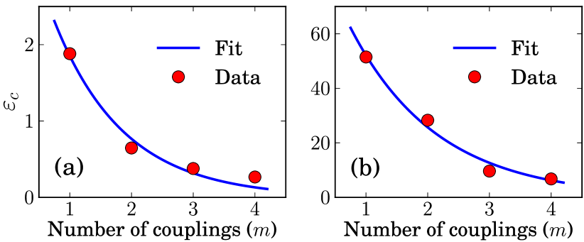
Figure 18: (color online) Critical coupling strength as a function of the number of additional couplings between the drive and the response array for a fixed number of oscillators in the array displaying an exponential decay of $\varepsilon_{c}$ as a function of number of additional couplings (a) Rössler and, (b) Lorenz system.

It may be noted that the critical coupling strength follows an exponential relation with the number of couplings as $\varepsilon_{c}\sim\varepsilon_{0}\exp(-\gamma\,m)$, with $m$ being the number of couplings. The constants, in the case of Rössler equations, turn out to be $\varepsilon_{0}=4.4746$ and $\gamma=0.8819$ while they are $\varepsilon_{0}=105.6375$ and $\gamma=0.7069$ for Lorenz equations.

IV Summary and conclusion

In this paper, we have studied chaos synchronization in arrays of diffusively coupled nonlinear oscillators with a ring geometry driven externally by an identical oscillator. In particular, we have shown that the critical coupling strength required to synchronize the array with the external drive increases exponentially with a scaling exponent $\gamma\in(0.3,0.5)$ as a function of the number $N_{c}$ of the oscillators in the array. We have pointed out that as a consequence of the exponential relation, the maximum number of oscillators in the array that can evolve in synchrony with the external drive is limited. Further, we have shown that by introducing additional couplings between the external drive and the array at $(mN_{c}+1)$-th oscillators in the ring, one can proportionately increase the maximum number of oscillators that can evolve in synchrony with the drive.

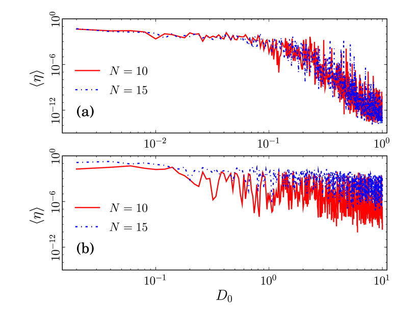
Figure 19: (color online) Time averaged synchronization error $\langle\eta\rangle$ for different numbers of oscillators in the ring as a function of noise intensity $D_{0}$ for the fixed value of $\varepsilon_{c}$ displaying power-law decay for (a) the Rössler oscillators in the range $D_{0}\in(0.01,1)$, and (b) the Lorenz oscillators in the range $D_{0}\in(0.01,10)$ with second additional coupling at the $N$-th and $2N$-th neighbor, respectively, of the first coupling.

Further, we have obtained the same exponential relation connecting the critical coupling strength and the number of oscillators even after introducing the additional number of couplings. Furthermore, we have found that $\varepsilon_{c}$ establishes an exponential decay as a function of the number of additional couplings between the drive and the response array for a fixed number of oscillators in the array. We have also examined the robustness of the results against noise of small intensity and found that the synchronization error displays a power law decay as a function of the noise intensity at $\varepsilon=\varepsilon_{c}$ indicating the existence of noise-enhanced and noise-induced synchronization for $\varepsilon<\varepsilon_{c}$ in all the cases.

In addition, we have also obtained similar results as above in other ubiquitous coupled nonlinear oscillators such as coupled MLC circuits, Chua’s circuits and Sprott oscillators as well, and also in a discrete system, namely coupled logistic maps, thus confirming the universality of the above results. One can also extend the same type of analysis with other coupling configurations such as star-type, unidirectional, global, weighted coupling configurations, 2-d, 3-d lattices, etc. We believe that our results shed more light on controllability and synchronizability of networks by introducing additional couplings at appropriate oscillators/nodes with the less cost in terms of the coupling strength. Further investigations can be extended to networks, in particular to network with community structure using pinning control and also with delay coupling.