Gang FTP scheduling of periodic
and parallel rigid real-time tasks

Abstract

In this paper we consider the scheduling of periodic and parallel rigid tasks. We provide (and prove correct) an exact schedulability test for Fixed Task Priority (FTP) Gang scheduler sub-classes: Parallelism Monotonic, Idling, Limited Gang, and Limited Slack Reclaiming. Additionally, we study the predictability of our schedulers: we show that Gang FJP schedulers are not predictable and we identify several sub-classes which are actually predictable. Moreover, we extend the definition of rigid, moldable and malleable jobs to recurrent tasks.

1 Introduction

We consider the preemptive scheduling of real-time tasks on identical multiprocessor platforms (see [2, 1]). We deal with parallel real-time tasks, the case where each job may be executed on different processors simultaneously, i.e., we allow job parallelism. Nowadays, the design of parallel programs is common thanks to parallel programming paradigms like Message Passing Interface (MPI [13, 14]) or Parallel Virtual Machine (PVM [18, 12]). Even better, sequential programs can be parallelized using tools like OpenMP (see [5] for details).

Related Work.

Few models and results in the literature concern hard real-time and parallel tasks. Manimaran et al. in [17] consider the non-preemptive EDF scheduling of periodic tasks. Han et al. in [15] considered the scheduling of a (finite) set of real-time jobs allowing job parallelism while we consider the scheduling of either infinite set of jobs or equivalently a set a periodic tasks. In previous work we contributed mainly to the feasibility problem of parallel tasks. In [6] we provided a task model which integrates job parallelism. We proved that the time-complexity of the feasibility problem of these systems is linear relatively to the number of (sporadic) tasks. More recently, we considered the scheduling of jobs which are composed of phases to be executed sequentially ; in [3] we provided a necessary feasibility test. Regarding the schedulability of recurrent real-time tasks, and to the best of our knowledge, we can only report the S. Kato et al. work (see [16] for details) which considers the Gang scheduling of rigid tasks (the number of processors is fixed beforehand) and provides a sufficient schedulability condition for Gang EDF scheduling.

This Research.

In this paper we study the scheduling of recurrent and parallel rigid tasks. Our main contribution is an exact schedulability test for Fixed Task Priority (FTP) Gang schedulers. Additionally, we study the predictability of our schedulers: we show that Gang FJP schedulers are not predictable and we identify several sub-classes which are actually predictable. Our technique is based on previous work for the scheduling of periodic tasks upon multiprocessors [8, 7]. To summarize the technique, we characterized for FTP schedulers and for asynchronous periodic task models, upper bounds of the first time-instant where the schedule repeats. Based on the upper bounds and the predictability property, we provide exact schedulability tests for asynchronous constrained deadline periodic task sets. The predictability property is important in the technique and will be revisited in this work. We also extend the definition of rigid, moldable and malleable jobs to recurrent tasks.

Paper Organization.

This paper is organized as follows. Section 2 introduces definitions, the model of computation and our assumptions. In Section 3 we study the predictability of our system, in particular we show that Gang FJP schedulers are not predictable and we identify several sub-classes which are actually predictable. We prove the periodicity of feasible schedules of periodic systems in Section 4. In Section 5 we combine the periodicity and predictability properties, to provide, for our Gang FTP sub-classes, an exact schedulability test. Lastly, we conclude in Section 6.

2 Model and Definitions

2.1 Parallel Terminology

The parallel literature [10, 4, 11] defines several kind of parallel tasks. But tasks in the non real-time parallel terminology does not have the same meaning as tasks in real-time scheduling literature. Actually, tasks in the parallel literature corresponds to jobs in our real-time community (i.e., corresponds to task instance). Especially, the notion of rigid recurrent task is not defined and does not extend trivially from the non real-time literature, in this section we fill the gap.

Definition 1 (Rigid, Moldable and Malleable Job).

A job is said to be:

Rigid

if the number of processors assigned to this job is specified externally to the scheduler a priori, and does not change throughout its execution;

Moldable

if the number of processors assigned to this job is determined by the scheduler, and does not change throughout its execution;

Malleable

if the number of processors assigned to this job can be changed by the scheduler during the job’s execution.

Definition 2 (Rigid, Moldable and Malleable Recurrent Task).

A periodic/sporadic task is said to be:

Rigid

if all its jobs are rigid, and the number of processors assigned to the jobs is specified externally to the scheduler;

Moldable

if all its jobs are moldable;

Malleable

if all its jobs are malleable.

Notice that a rigid task does not necessarily have jobs with the same size. For instance, if the user/application decides that odd instances require $v$ processors, and even instances $v^{\prime}$ processors, the task is said to be rigid.

2.2 Task and Job Model

We consider the preemptive scheduling of parallel jobs on a multiprocessor platform with $m$ processors. We will focus on the problem of scheduling a set of parallel jobs, each job $J_{j}\stackrel{{\scriptstyle\mathrm{def}}}{{=}}(r_{j},v_{j},e_{j},d_{j})$ is characterized by a release time $r_{j}$, $v_{j}$ a required number of processors, an execution requirement $e_{j}$ and an absolute deadline $d_{j}$. The job $J_{j}$ must execute for $e_{j}$ time units over the interval $[r_{j},d_{j})$ on $v_{j}$ processors. We consider the scheduling of rigid tasks since $v_{i}$ is fixed externally to the scheduler. Actually, S. Kato et al. in [16] have the same assumption as we do, and, given the Definition 2, they consider rigid tasks, and not moldable tasks, as said in their paper — otherwise the scheduler would determine $v_{i}$ on-line and at job-level.

As we will consider periodic systems, let $\tau=\{\tau_{1},\ldots,\tau_{n}\}$ denote a set of $n$ periodic parallel tasks. Each task $\tau_{i}=(O_{i},v_{i},C_{i},D_{i},T_{i},)$ will generate an infinite number of jobs, where the $k^{\text{th}}$ job of task $\tau_{i}$ is

$$(O_{i}+(k-1)T_{i},v_{i},C_{i},O_{i}+(k-1)T_{i}+D_{i}).$$

The execution requirement of a job of $\tau_{i}$ corresponds as a $C_{i}\times v_{i}$ rectangle. In this document we assume $D_{i}\leq T_{i}$ for any $\tau_{i}$, i.e., we consider constrained deadline systems. We consider multiprocessor platforms $\pi$ composed of $m$ identical processors: $\{\pi_{1},\pi_{2},\ldots,\pi_{m}\}$.

2.3 Priority Assignment and Schedulers

In this document we consider FTP and FJP schedulers with the following definitions.

Definition 3 (FTP).

A priority assignment is a Fixed Task Priority assignment if it assigns the priorities to the tasks beforehand; at run-time each job priority corresponds to its task priority. (An FTP scheduler uses an FTP priority assignment.)

We assume that tasks are indexed according to priority (lower the index, higher the priority).

Definition 4 (FJP).

A priority assignment is a Fixed Job Priority assignment if and only if it satisfies the condition that: for every pair of jobs $J_{i}$ and $J_{j}$, if $J_{i}$ has higher priority than $J_{j}$ at some time-instant, then $J_{i}$ always has higher priority than $J_{j}$. (An FJP scheduler uses an FJP priority assignment.)

Remark that any FTP assignment is also FJP.

Definition 5 (Gang FJP).

At each instant, the algorithm schedules jobs on processors as follows: the highest priority (active) job $J_{i}$ is scheduled on the first $v_{i}$ available processors (if any). The very same rule is then applied to the remaining active jobs on the remaining available processors.

Priority inversion.

Figure 1 illustrates the Gang FTP schedule ($\tau_{1}$ is the highest priority task and $\tau_{3}$ the lowest one) of $\tau_{1}=(0,2,2,5,5),\tau_{2}=(0,2,3,5,5),\tau_{3}=(0,1,4,5,5)$. Notice that Gang FJP and FTP can produce schedules where a lower-priority job ($J_{j}$) is scheduled while an active higher-priority job ($J_{i}$) is not (typically if $v_{i}>v_{j}$ — which occurs at time $0$ in our example, $\tau_{2}$ and $\tau_{3}$ are active, $\tau_{3}$ is executing in $[0,2)$ while $\tau_{2}$ is not). This phenomenon, called priority inversion in this document, could be a drawback as we will see. Fortunately, we keep an important FTP-property: the scheduling of the sub-set $\{\tau_{1},\ldots,\tau_{i}\}$ is not jeopardized by lower-priority tasks ($\{\tau_{i+1},\ldots,\tau_{n}\}$).

Figure 1: Gang FTP schedule with priority inversion at time $0$.

Definition 6 (Schedule $\sigma(t)$).

For any set of jobs $J\stackrel{{\scriptstyle\mathrm{def}}}{{=}}\{J_{1},J_{2},J_{3},\ldots\}$ and any set of $m$ identical processors $\{\pi_{1},\ldots,\pi_{m}\}$ we define the schedule $\sigma(t)$ of system $\tau$ at time-instant $t$ as $\sigma:\mathbb{N}\rightarrow\mathbb{N}^{m}$ where $\sigma(t)\stackrel{{\scriptstyle\mathrm{def}}}{{=}}(\sigma_{1}(t),\sigma_{2}(t),\ldots,\sigma_{m}(t))$ with
$\sigma_{j}(t)\stackrel{{\scriptstyle\mathrm{def}}}{{=}}\left\{\begin{array}[]{ll}0,&\text{if there is no job scheduled on }\pi_{j}\\ &\text{at time-instant }t;\\ i,&\text{if job }J_{i}\mbox{ is scheduled on }\pi_{j}\text{ at}\\ &\text{time-instant }t.\end{array}\right.$

Definition 7 (Availability of the processors).

For any ordered set of jobs $J$ and any set of $m$ processors $\{\pi_{1},\ldots,\pi_{m}\}$, we define the availability of the processors $A(J,t)$ of the set of jobs $J$ at time-instant $t$ as the set of available processors: $A(J,t)\stackrel{{\scriptstyle\mathrm{def}}}{{=}}\{j\mid\mbox{ }\sigma_{j}(t)=0\}$, where $\sigma$ is the schedule of $J$.

Definition 8 (Active, Ready and Running jobs).

A job is said to be active if it has been released, but is not finished yet. An active job is ready if it is not currently served ; an active job is running otherwise.

3 Predictability of Gang Scheduling

We consider the scheduling of sets of job $J\stackrel{{\scriptstyle\mathrm{def}}}{{=}}J_{1},J_{2},J_{3}\ldots$, (finite or infinite set of jobs) and without loss of generality we consider jobs in a decreasing order of priorities $(J_{1}>J_{2}>J_{3}>\cdots$). We suppose that the execution time of each job $J_{i}$ can be any value in the interval $[e_{i}^{-},e_{i}^{+}]$ and we denote by $J^{+}_{i}$ the job defined as $J^{+}_{i}\stackrel{{\scriptstyle\mathrm{def}}}{{=}}(r_{i},v_{i},e_{i}^{+},d_{i})$. We denote by $J^{(i)}$ the set of the first $i$ higher priority jobs. We denote also by $J^{(i)}_{-}$ the set $\{J^{-}_{1},\ldots,J^{-}_{i}\}$ and by $J^{(i)}_{+}$ the set $\{J^{+}_{1},\ldots,J^{+}_{i}\}$. Let $S(J)$ be the time-instant at which the lowest priority job of $J$ begins its execution in the schedule. Similarly, let $F(J)$ be the time-instant at which the lowest priority job of $J$ completes its execution in the schedule.

Definition 9 (Predictable algorithms).

A scheduling algorithm is said to be predictable if $S(J^{(i)}_{-})\leq S(J^{(i)})\leq S(J^{(i)}_{+})$ and $F(J^{(i)}_{-})\leq F(J^{(i)})\leq F(J^{(i)}_{+})$, for all $i\geq 1$ and for all schedulable $J^{(i)}_{+}$ sets of jobs.

Notice that the predictability of an algorithm implies that any system schedulable when all tasks use their worst case execution time is also schedulable when a task takes less time than expected. We then just need to show that the system is schedulable in the worst case to prove that the system is schedulable in all scenarios.

In previous work [9] we proved, for a quite general model, i.e., FJP priority schedulers on unrelated multiprocessors, the predictability for sequential jobs (i.e., $v_{i}=1$ for any $J_{i}$). Unfortunately that property is not satisfied for parallel jobs.

Lemma 10.

Gang FJP schedulers are not predictable on multiprocessors.

Figure 2: Non-predictability of Gang FJP schedulers. $1>2>3$, and they all arrive at time $0$.

Proof.

Here is an example task system, on 2 processors (see Figure 2):

$$J_{1}=(0,1,3,3),J_{2}=(0,2,1,4),J_{3}=(0,1,2,2)\enspace.$$

Upon two processors and using the priority assignment $J_{1}>J_{2}>J_{3}$, Gang FJP schedules the set of jobs ($J_{3}$ completes at time-instant 2). Unfortunately, if the actual duration of $J_{1}$ is 1, $J_{2}$ will preempt $J_{3}$ at time $t=1$ and $J_{3}$ will complete later, at time-instant 3. Then, $J_{3}$ does not miss its deadline in the “worst case” scenario, but misses it if $J_{1}$ uses less than its worst case execution time $e_{1}$. ∎

This negative result implies that neither the DM, RM nor EDF are predictable for Gang scheduling.

The problem we highlight in this example occurs because some jobs which were not preempted in the worst case scenario are preempted in a scenario with shorter execution times. In other words, by allowing a job $J_{i}$ taking advantage of some slack time given by another (higher priority) job, $J_{i}$ interrupts a job $J_{j}$ (with $J_{j}<J_{i}$) which would not have been suspended if we did not have any slack.

If, as we will do and prove in this work, we find a way to avoid the priority inversion phenomenon, we will never have those problematic preemptions. Indeed, if no lower priority job $J_{j}$ is authorized to start between the arrival of $J_{i}$ ($J_{j}<J_{i}$) and its start time, then if $J_{i}$ starts anywhere between its arrival time, and its start time in the worst case scenario, it will not interrupt tasks that it would not have interrupt in the worst case.

The “problematic preemptions” can be avoided by (at least) three ways:

• By avoiding the priority inversion;

• By avoiding any slack (or by not using it);

• By using the slack, but in a “smart” way.

In order to obtain a predictable system, we identify two ways of modifying the system:

• First, we will propose to constraint the priority assignment. We introduce the Parallelism Monotonic FTP assignment, and prove the predictability of these priority assignments;

• Second, we will propose three variants of the scheduler, giving a predictable behavior. Those variants are the idling scheduler (not using the slack), the limited Gang FJP scheduler (avoiding priority inversion), and the Gang FJP scheduler with limited slack reclaiming (smartly using the slack).

3.1 Parallelism Monotonic FTP Assignment

In this section we will consider a sub-class of Gang FTP assignments which are predictable.

Definition 11 (Parallelism Monotonic).

An FTP priority assignment is Parallelism Monotonic iff $i<j\Rightarrow v_{i}\leq v_{j}$.

Notice that this class is very interesting from the theoretical point of view, but might be not a good choice for some implementation. Indeed, it gives a low priority to highly parallel jobs, which makes them more difficult to schedule. In general, it might be useful to first schedule the very parallel jobs, and then to fill the available processors with smaller jobs.

We will now prove that any Parallelism Monotonic assignment are predictable.

In [9] we showed that $A(J^{(i)}_{+},t)\subseteq A(J^{(i)},t)$, for all $t$ and all $i$. In other words, that at any time-instant the processors available in ${\sigma^{(i)}_{+}}$ are also available in ${\sigma^{(i)}}$. The counterexample used in the proof of Lemma 10 violates that property as well. In the following we will consider another kind of processors availability.

Definition 12 (Level-($i$) availability of the processors).

For any ordered set of $i-1$ jobs $J=J_{1},\ldots,J_{i-1}$ and any set of $m$ processors, we define the level-($i$) availability of the processors $A_{i}(J,t)$ of the set of jobs $J$ at time-instant $t$ as follows

$$A_{i}(J,t)\stackrel{{\scriptstyle\mathrm{def}}}{{=}}\begin{cases}\#A(J,t)&\text{if $\#A(J,t)\geq v_{i}$};\\ 0&\text{otherwise}.\end{cases}$$

Informally speaking, $A_{i}(J,t)$ is the the number of available processors if the latter is sufficient to schedule $J_{i}$, otherwise $A_{i}(J,t)$ is null.

Lemma 13.

For any schedulable ordered set of jobs $J$, using a Gang FJP Parallelism Monotonic on $m$ processors, we have $A_{i}(J^{(i-1)}_{+},t)\leq A_{i}(J^{(i-1)},t)$, for all $t$ and all $i$. (We consider that the sets of jobs are ordered in the same decreasing order of the priorities, i.e., $J_{1}>J_{2}>\cdots>J_{\ell}$ and $J_{1}^{+}>J_{2}^{+}>\cdots>J_{\ell}^{+}$.)

Proof.

The proof is made by induction on $\ell$ (the number of jobs). Our inductive hypothesis is the following: $A_{k}(J^{(k-1)}_{+},t)\leq A_{k}(J^{(k-1)},t)$, for all $t$ and $1<k\leq i+1$.

The property is true in the base case since $A_{2}(J^{(1)}_{+},t)\leq A_{2}(J^{(1)},t)$, for all $t$. Indeed, $S(J^{(1)})=S(J^{(1)}_{+})$. Moreover $J_{1}$ and $J_{1}^{+}$ are both scheduled on the (same) first $v_{1}$ processors, but $J_{1}^{+}$ will be executed for the same or a greater amount of time than $J_{1}$.

We will show now that $A_{i+2}(J^{(i+1)}_{+},t)\leq A_{i+2}(J^{(i+1)},t)$, for all $t$.

Since the jobs in $J^{(i)}$ have higher priority than $J_{i+1}$, then the scheduling of $J_{i+1}$ will not interfere with higher priority jobs which have already been scheduled. Similarly, $J^{+}_{i+1}$ will not interfere with higher priority jobs of $J^{(i)}_{+}$ which have already been scheduled. Therefore, we may build the schedule $\sigma^{(i+1)}$ from $\sigma^{(i)}$, such that the jobs $J_{1},J_{2},\ldots,J_{i}$, are scheduled at the very same instants and on the very same processors as they were in $\sigma^{(i)}$. Similarly, we may build $\sigma^{(i+1)}_{+}$ from $\sigma^{(i)}_{+}$.

Note that property is straightforward for time-instants where $J^{(i+1)}$ is not scheduled since the processor availability is not modified and by definition of level-($i+2$) processor availability.

We will consider time-instant $t$, from $r_{i+1}$ to the completion of $J_{i+1}$ (which is actually not after the completion of $J_{i+1}^{+}$, see below for a proof), we distinguish between three cases:

1. $A_{i+1}(J^{(i)}_{+},t)=A_{i+1}(J^{(i)},t)=0$: in both situations no enough processors are available for $J_{(i)}$ (and $J_{(i)}^{+}$). Therefore, both jobs, $J_{i+1}$ and $J_{i+1}^{+}$, do not progress and we obtain $A_{i+2}(J^{(i+1)}_{+},t)=A_{i+2}(J^{(i)}_{+},t)=A_{i+2}(J^{(i+1)},t)=A_{i+2}(J^{(i)},t)=0$, since $v_{i+2}\geq v_{i+1}$. The progression of $J_{i+1}$ is identical to $J_{i+1}^{+}$.

2. $0=A_{i+1}(J^{(i)}_{+},t)<v_{i+1}\leq A_{i+1}(J^{(i)},t)$: $J_{i+1}$ progress on the $v_{i+1}$ first available processors in $A(J^{(i)},t)$ (not available in $A(J^{(i)}_{+},t)$). $J_{i+1}^{+}$ does not progress. $A_{i+2}(J^{(i)}_{+},t)=0$ since $v_{i+2}\geq v_{i+1}$. The progression of $J_{i+1}$ is strictly larger than $J_{i+1}^{+}$.

3. $v_{i+1}\leq A_{i+1}(J^{(i)},t)\leq A_{i+1}(J^{(i)}_{+},t)$, $J_{i+1}$ and $J_{i+1}^{+}$ progress on the same processors. The property follows by induction hypothesis.

Therefore, we showed that $A_{i+2}(J^{(i+1)}_{+},t)\leq A_{i+2}(J^{(i+1)},t)$, for all $t$, from $r_{i+1}$ to the completion of $J_{i+1}$ and that $J_{i+1}$ does not complete after $J_{i+1}^{+}$. For the time-instant after the completion of $J_{i+1}$ the property is trivially true by induction hypothesis. ∎

Theorem 14.

Gang FJP schedulers are predictable on identical platforms with Parallelism Monotonic priority assignment.

Proof.

In the framework of the proof of Lemma 13 we actually showed extra properties which imply that Gang FJP Parallelism Monotonic schedulers are predictable on identical platforms: (i) $J_{i+1}$ completes not after $J_{i+1}^{+}$ and (ii) $J_{i+1}$ can be scheduled either at the very same instants as $J_{i+1}^{+}$ or may progress during additional time-instants (case (2) of the proof) these instants may precede the time-instant where $J_{i+1}^{+}$ commences its execution. ∎

3.2 Idling Scheduler

Instead of giving constraints on the priority assignment, we can also adapt our scheduler in order to make it predictable. A first way of doing that is to force tasks to run exactly up to their worst case. If a task does not use its worst case, then the scheduler idles the processor(s) up to the expected end time.

Definition 15 (Idling scheduler).

An idling scheduler idles any processor that was used by a task which finished earlier than its worst case, up to the time the processor would have been released in the worst case scenario.

Lemma 16.

Gang FJP Idling schedulers are predictable on identical platforms.

Proof.

The proof is very straightforward in this case: any task starts at the same time in the worst case $J^{+}$, and in the case where some tasks use less than than their worst case. And if we consider the completion time of a job as the time at which its (possibly empty) idle period finishes, then the end time will be the same in the worst case scenario as in any case. Then,

$$S(J^{(i)}_{-})\leq S(J^{(i)})\leq S(J^{(i)}_{+}),$$

and

$$F(J^{(i)}_{-})\leq F(J^{(i)})\leq F(J^{(i)}_{+}).$$

∎

3.3 Limited Gang FJP Scheduler

The predictability can also be ensured if we avoid the priority inversion phenomenon reported in Section 1, more precisely by restricting Gang FTP/FJP as follows:

Definition 17 (Limited Gang FJP scheduler).

At each instant, the algorithm schedules jobs on processors as follows: the highest priority (active) job $J_{i}$ is scheduled on the first $v_{i}$ available processors (if any). The very same rule is then applied to the remaining active jobs on the remaining available processors only if $J_{i}$ was scheduled (i.e., if at least $v_{i}$ processors were available).

We now prove that limited Gang FJP are predictable but first an additional definition.

Definition 18 (Limited level-($i$) availability of the processors).

For any ordered set of $i-1$ jobs $J=J_{1},\ldots,J_{i-1}$ and any set of $m$ processors, we define the limited level-($i$) availability of the processors $\hat{A}_{i}(J,t)$ of the set of jobs $J$ at time-instant $t$ as follows ($\hat{A}_{0}(J,t)=m$ for all $J,t$):

$$\hat{A}_{i}(J,t)\stackrel{{\scriptstyle\mathrm{def}}}{{=}}\begin{cases}0&\text{if $\hat{A}_{i-1}(J,t)=0$};\\ \#A(J,t)&\text{if }\#A(J,t)\geq v_{i}\text{ and }\\ &\hat{A}_{i-1}(J,t)\neq 0;\\ 0&\text{otherwise.}\end{cases}$$

Lemma 19.

For any schedulable ordered set of jobs $J$, using a Limited Gang FJP on $m$ processors, we have $\hat{A}_{i}(J^{(i-1)}_{+},t)\leq\hat{A}_{i}(J^{(i-1)},t)$, for all $t$ and all $i$. (We consider that the sets of jobs are ordered in the same decreasing order of the priorities, i.e., $J_{1}>J_{2}>\cdots$ and $J_{1}^{+}>J_{2}^{+}>\cdots$.)

Proof.

The property follows using a similar reasoning as the proof of Lemma 13 and the fact that $\hat{A}_{i}(J^{(i-1)},t)\geq\hat{A}_{i+1}(J^{(i-1)},t).$ ∎

Theorem 20.

Limited Gang FJP schedulers are predictable on identical platforms.

Proof.

The proof is similar to the proof given for Theorem 14. $\hat{A}_{i}(J^{(i-1)},t)$ describes the number of processors available to schedule $J_{i}$. As this number is at any time higher in $J_{+}^{(i-1)}$ than in $J^{(i-1)}$, then $J_{i}$ will never start later in $J^{(i-1)}$ than in $J_{+}^{(i-1)}$, and will never finish later either. ∎

Remark that by using limited Gang scheduling we accept to lose efficiency in the resource utilization to ensure system predictability.

3.4 Gang FJP and Limited Slack Reclaiming

As highlighted previously, the problem of using the slack caused by a job finishing earlier than expected is that it could cause a preemption that would not have occurred if the job had used its worst case execution time. But with a closer look, we can see that the problem only occurs when a job $J_{i}$ wider than a job $J_{j}$ ($v_{i}>v_{j}$) takes advantage of the slack created by $J_{j}$ early completion. A way of avoiding this is to only allow job not larger than the early completed job to use the slack. This is what we propose in this technique.

Definition 21 (Slack server).

A slack server of level $\ell$, width $w$ and length $\lambda$ is a job of priority $\ell$, on $w$ processors, running for $\lambda$ units of time, serving jobs with a priority lower than $\ell$ which do not require more than $w$ processors. If no task are available, the server stays idle until the end of the $\lambda$ units of time.

It may be noticed that:

• We do not give any constraint about the way the “slack server scheduling” (the way jobs are scheduled inside the slack server) is performed;

• Within a slack server, we might run several jobs in parallel, as long as they never need more than $w$ processors simultaneously;

• If a job being served by the slack server becomes eligible by the “global scheduler”, then it should be interrupted in the slack server, and made available to the global scheduler;

• All jobs served by the slack server should still stay in the ready state (but not running) from the “global scheduler” point of view.

Regarding this definition of a slack server, we can now define how our schedule will work.

Definition 22 (Gang FJP and limited slack reclaiming).

A Gang FJP scheduler with limited slack reclaiming, works as follows: At each scheduling point (the completion of a job or an arrival):

• If this corresponds to the end of a job $J_{i}$, and this job used $e^{\prime}<e_{i}$ units of time, starts a slack server of level $i$, width $v_{i}$, length $e_{i}-e^{\prime}$;

• Otherwise, the highest priority (active) job $J_{i}$ is scheduled on the first $v_{i}$ available processors (if any). The very same rule is then applied to the remaining active jobs on the remaining available processors.

We can make an important observation about this scheduling algorithm. Jobs that are run in the slack server will not have any other impact on the global scheduler that reducing the execution time of those jobs. So if we consider the slack server as a black box, the schedule will be exactly the same as if this black box was just idling. The only impact will be the proportion between actual and worst case execution time.

Remark also that will we cause priority inversion: some jobs will be run inside the slack server, while other higher priority ready job (but wider than the slack server) will be kept suspended.

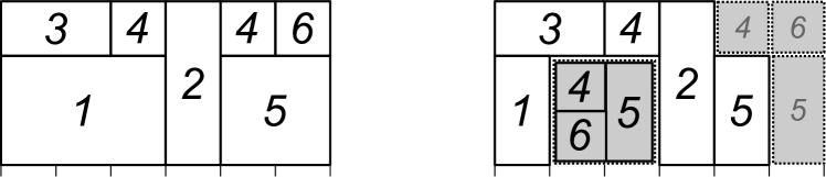
Figure 3: Slack server example. Left: all jobs use their worst case execution time. Right: Job 1 is shorter than expected, and a slack server is set up (gray part).

Figure 3 illustrates how the slack server works. We consider the following set of jobs (they all have the same arrival time $0$, and the same deadline $6$:

	$J_{1}$	$J_{2}$	$J_{3}$	$J_{4}$	$J_{5}$	$J_{6}$
$v_{i}$	2	3	1	1	2	1
$e_{i}$	3	1	2	2	2	1

The left side of Figure 3 shows the schedule where all jobs use their worst case execution time. On the right side, $J_{1}$ finishes at time $1$ (instead of $3$). The schedulers launches then a slack server (in gray on the figure) of level $1$, width $2$ and length $2$, in order to fill the space that would have been used by $J_{1}$ in the worst case scenario. This server is then scheduled as a job of priority $1$, as was $J_{1}$. At time $1$, the slack server sees that jobs $J_{2}$, $J_{4}$, $J_{5}$, $J_{6}$ are ready ($J_{3}$ is running). But $J_{2}$ is too wide, so the slack server can for instance choose (arbitrarily) to run $J_{4}$ and $J_{6}$. After one unit of time, the scheduler sees that it can run $J_{4}$, the highest priority task which can run on the only available processor released by the end of $J_{3}$. $J_{4}$ is then “preempted” inside the slack server, and run normally. Then the slack server choses to run $J_{5}$ ($J_{6}$ is done). At time $3$, the slack server ends, and $J_{5}$ is preempted.

At time $4$ and $5$, we need to start slack servers for $J_{4}$, $J_{5}$ and $J_{6}$, but they do not receive any work to perform.

Remark that if we compare both schedules of Figure 3, and see the slack server as part of the concerned job, all tasks start end and at the same time in both scenarios.

Theorem 23.

Gang FJP schedulers with limited slack reclaiming are predictable on identical platforms.

Proof.

From the schedulability point of view, this behaves exactly the same way as the Idling server. But instead of being idle, the slack server decreases the actual execution time of some ready (but not running) jobs.

One job will never preempt a job that would not have been preempted in the worst case scenario. ∎

Notice that with this kind of scheduler, we might considered the system as being not fully FTP anymore. Some jobs are indeed eligible (enough resource to run them), but are left waiting. In the presentation of this section, we said that we did not give any constraint on the scheduler of the slack server. Indeed, the method we use does not have any impact on the predictability of the system. But we can of course use a FTP scheduling algorithm. This does not make the global system to be strictly FTP, but it makes closer.

Notice also that we present a system with two level of scheduler: one global, and one inside the slack server. This distinction was used for the sake of presentation, but in a real implementation, the global scheduler can of course also do the job of the slack server scheduler.

4 Periodicity

In this section we prove the periodicity of feasible Gang FTP schedules. It is important to note that we assume in this section that each job of the same task (say $\tau_{i}$) has an execution requirement which is exactly $C_{i}$ time units. Thanks to the predictability property this situation corresponds to the worst case.

Remark that, as we consider only the case where all job has its worst case, the schedule of an idling, slack reclaiming or general scheduler is exactly the same.

Theorem 24.

For any preemptive (limited or not) Gang FTP algorithm $\mathcal{A}$, if an asynchronous constrained deadline system $\tau$ is $\mathcal{A}$-feasible, then the $\mathcal{A}$-feasible schedule of $\tau$ on $m$ identical processors is periodic with a period $P\stackrel{{\scriptstyle\mathrm{def}}}{{=}}\mathrm{lcm}\{T_{1},\ldots,T_{n}\}$ from instant $S_{n}$ where $S_{i}$ is defined inductively as follows:

• $S_{1}\stackrel{{\scriptstyle\mathrm{def}}}{{=}}O_{1}$;

• $S_{i}\stackrel{{\scriptstyle\mathrm{def}}}{{=}}\max\{O_{i},O_{i}+\left\lceil\dfrac{S_{i-1}-O_{i}}{T_{i}}\right\rceil T_{i}\},\forall i\in\{2,3,\ldots,n\}$.

(Assuming that the execution time of each task is constant.)

Proof.

The proof is made by induction on $n$ (the number of tasks). We denote by $\sigma^{(i)}$ the schedule obtained by considering only the task subset $\tau^{(i)}$, the first higher priority $i$ tasks $\{\tau_{1},\ldots,\tau_{i}\}$, and by $A(J^{(i)},t)$ the corresponding availability of the processors. Our inductive hypothesis is the following: the schedule $\sigma^{(k)}$ is periodic from $S_{k}$ with a period $P_{k}\stackrel{{\scriptstyle\mathrm{def}}}{{=}}\mathrm{lcm}\{T_{1},\ldots,T_{k}\}$ for all $1\leq k\leq i$.

The property is true in the base case: $\sigma^{(1)}$ is periodic from $S_{1}=O_{1}$ with period $P_{1}$, for $\tau^{(1)}=\{\tau_{1}\}$: since we consider (feasible) constrained deadline systems, at instant $P_{1}=T_{1}$ the previous request of $\tau_{1}$ has finished its execution and the schedule repeats.

We shall now show that any $\mathcal{A}$-feasible schedule of $\tau^{(i+1)}$ is periodic with period $P_{i+1}$ from $S_{i+1}$.

Since $\sigma^{(i)}$ is periodic with a period $P_{i}$ from $S_{i}$ the following equation is verified:

$$\sigma^{(i)}(t)=\sigma^{(i)}(t+P_{i}),\forall t\geq S_{i}.$$ (1)

We denote by $S_{i+1}\stackrel{{\scriptstyle\mathrm{def}}}{{=}}\max\{O_{i+1},O_{i+1}+\left\lceil\dfrac{S_{i}-O_{i+1}}{T_{i+1}}\right\rceil T_{i+1}\}$ the first request of $\tau_{i+1}$ not before $S_{i}$.

Since the tasks in $\tau^{(i)}$ have higher priority than $\tau_{i+1}$, then the scheduling of $\tau_{i+1}$ will not interfere with higher priority tasks which are already scheduled. Therefore, we may build $\sigma^{(i+1)}$ from $\sigma^{(i)}$ such that the tasks $\tau_{1},\tau_{2},\ldots,\tau_{i}$ are scheduled at the very same instants and on the very same processors as they were in $\sigma^{(i)}$. We apply now the induction step: for all $t\geq S_{i}$ in $\sigma^{(i)}$ we have $A(J^{(i)},t)=A(J^{(i)},t+P_{i})$ the availability of the processors repeats. Notice that at those instants $t$ and $t+P_{i}$ the available processors (if any) are the same. Consequently at only these instants where $\#A(J^{(i)},t)\geq v_{i+1}$, task $\tau_{i+1}$ may be executed. Notice that the scheduler can decide to leave one or several processor(s) to be idle intentionally in a deterministic and memoryless way. Notice also, in the “non limited case”, that $\tau_{i+1}$ might start executing before a higher priority task $\tau_{j}$ (with $j<i+1$), if $v_{j}>\#A(J^{(i)},t)>v_{i+1}$. But as soon as $v_{j}$ processors are available in $A(J^{(i)},t)$, $\tau_{i+1}$ is preempted (if still running) and the CPU is given to $\tau_{j}$.

The instants $t$ with $S_{i+1}\leq t<S_{i+1}+P_{i+1}$, where $\tau_{i+1}$ may be executed in $\sigma^{(i+1)}$, are periodic with period $P_{i+1}$ since $P_{i+1}$ is a multiple of $P_{i}$. Moreover since the system is feasible and we consider constrained deadlines, the only active request of $\tau_{i+1}$ at $S_{i+1}$, respectively at $S_{i+1}+P_{i+1}$, is the one activated at $S_{i+1}$, respectively at $S_{i+1}+P_{i+1}$. Consequently, the instants at which the deterministic and memoryless algorithm $\mathcal{A}$ schedules $\tau_{i+1}$ are periodic with period $P_{i+1}$. Therefore, the schedule $\sigma^{(i+1)}$ repeats from $S_{i+1}$ with period equal to $P_{i+1}$ and the property is true for all $1\leq k\leq n$, in particular for $k=n:$ $\sigma^{(n)}$ is periodic with period equal to $P$ from $S_{n}$ and the property follows. ∎

5 Exact Schedulability Test

Now we have the material to define an exact schedulability test for rigid and asynchronous periodic systems.

Corollary 25.

For any preemptive Gang FTP predictable algorithm $\mathcal{A}$ (i.e., Parallelism Monotonic, Idling, Limited Gang, and Limited Slack Reclaiming variants) and for any asynchronous rigid constrained deadline system $\tau$ on $m$ identical processors, $\tau$ is $\mathcal{A}$-schedulable if and only if

• all deadlines are met in $[0,S_{n}+P)$ and

• $\theta(S_{n})=\theta(S_{n}+P)$

where $S_{i}$ are defined inductively in Theorem 24.

Proof.

Corollary 25 is a direct consequence of Theorem 24 and the predictability of Parallelism Monotonic (Theorem 14), Idling (Lemma 16), Limited Gang (Theorem 20), and Limited Slack Reclaiming (Theorem 23) variants. ∎

6 Conclusion and Future Work

In this paper we considered the scheduling of periodic and parallel rigid tasks. We provided and proved correct an exact schedulability test for Fixed Task Priority (FTP) Gang scheduler sub-classes: Parallelism Monotonic, Idling, Limited Gang, and Limited Slack Reclaiming. Additionally, we studied the predictability of our schedulers: we show that Gang FJP schedulers are not predictable and we identify several sub-classes which are actually predictable. We also extended the definition of rigid, moldable and malleable jobs to recurrent tasks.

In future work we aim to extend the model by considering moldable tasks — task can be executed in a varying number of processors — that is the scheduler can determine, on-line, the rectangle of each task instance (job) based upon parallel performance model (e.g., the one defined in [6]).

References

- [1] Baker, T. P. An analysis of EDF scheduling on a multiprocessor. IEEE Trans. on Parallel and Distributed Systems 15, 8 (2005), 760–768.
- [2] Baker, T. P., and Baruah, S. Schedulability analysis of multiprocessor sporadic task systems. Handbook of Real-Time and Embedded Systems (2006).
- [3] Berten, V., Collette, S., and Goossens, J. Feasibility test for multi-phase parallel real-time jobs. In Proceedings of the Work-in-Progress session of the IEEE Real-Time Systems Symposium 2009 (2009), D. Zhu, Ed., pp. 33–36.
- [4] Buyya, R. High Performance Cluster Computing: Architectures and Systems. Prentice Hall PTR, Upper Saddle River, NJ, USA, 1999, ch. Scheduling Parallel Jobs on Clusters, pp. 519–533.
- [5] Chandra, R., Dagum, L., Kohr, D., Maydan, D., McDonald, J., and Menon, R. Parallel programming in OpenMP. Morgan Kaufmann Publishers Inc., San Francisco, CA, USA, 2001.
- [6] Collette, S., Cucu, L., and Goossens, J. Integrating job parallelism in real-time scheduling theory. Information Processing Letters 106, 5 (May 2008), 180–187.
- [7] Cucu, L., and Goossens, J. Feasibility intervals for fixed-priority real-time scheduling on uniform multiprocessors. Proceedings of the 11th IEEE International Conference on Emerging Technologies and Factory Automation (2006), 397–405.
- [8] Cucu, L., and Goossens, J. Feasibility intervals for multiprocessor fixed-priority scheduling of arbitrary deadline periodic systems. Proceedings of the 10th Design, Automation and Test in Europe (2007), 1635–1640.
- [9] Cucu-Grosjean, L., and Goossens, J. Predictability of fixed-job priority schedulers on heterogeneous multiprocessor real-time systems. Information Processing Letters 110 (2010), 399–402.
- [10] Drozdowski, M. Scheduling parallel tasks — algorithms and complexity. Handbook of Scheduling (2005), 25–1–25–25.
- [11] Feitelson, D. G., and Rudolph, L. Toward convergence in job schedulers for parallel supercomputers. In Job Scheduling Strategies for Parallel Processing (1996), Springer-Verlag, pp. 1–26.
- [12] Geist, A., Beguelin, A., Dongarra, J., Jiang, W., Manchek, R., and Sunderam, V. PVM: Parallel Virtual Machine A Users’ Guide and Tutorial for Networked Parallel Computing. MIT Press, 1994.
- [13] Gorlatch, S., and Bischof, H. A generic MPI implementation for a data-parallel skeleton: Formal derivation and application to FFT. Parallel Processing Letters 8, 4 (1998), 447–458.
- [14] Gropp, W., Ed. Using MPI: portable parallel programming with the message-passing interface, 2nd ed. Cambridge, MIT Press, 1999.
- [15] Han, C., and Lin, K.-J. Scheduling parallelizable jobs on multiprocessors. Proceedings of the 10th IEEE Real-Time Systems Symposium (RTSS’89) (1989), 59–67.
- [16] Kato, S., and Ishikawa, Y. Gang EDF scheduling of parallel task systems. In 30th IEEE Real-Time Systems Symposium (2009), IEEE Computer Society, pp. 459–468.
- [17] Manimaran, G., Siva Ram Murthy, C., and Ramamritham, K. A new approach for scheduling of parallelizable tasks in real-time multiprocessor systems. Real-Time Systems 15 (1998), 39–60.
- [18] Sunderam, V. PVM: A framework for parallel distributed computing. Concurrency: Practice and Experience 2, 4 (1990), 315–339.