INSTITUT NATIONAL DE RECHERCHE EN INFORMATIQUE ET EN AUTOMATIQUE

ESS for life-history traits of cooperating consumers facing cheating mutants
P. Bernhard — F. Grognard — L. Mailleret — A.R. Akhmetzhanov N° 7314
June 2010

Abstract: We consider a population of identical individuals preying on an exhaustible resource. The individuals in the population choose a strategy that defines how they use their available time over the course of their life for feeding, for reproducing (say laying eggs), or split their energy in between these two activities. We here suppose that their life lasts a full season, so that the chosen strategy results in the production of a certain number of eggs laid over the season. This number then helps define the long-run evolution of the population since the eggs constitute the basis for the population for the next season. However, in this paper, we strictly concentrate on what occurs within a season, by considering two possible strategies: the collective optimum and the uninvadable strategy.

The (collective) optimal strategy involves a singular arc, which has some resource saving feature and may, on the long-term, lead to an equilibrium. However, it is susceptible to invasion by a greedy mutant which free-rides on this resource saving strategy. Therefore, the “optimal” strategy is not evolutionarily stable.

We thus look for an evolutionarily stable strategy, using the first ESS condition (“Nash-Wardrop condition”). This yields a different singular arc and a strategy that conserves less the resource. Unfortunately, we show in a forthcoming paper that, though it is an ESS, it is not long-term (interseasonal) sustainable. This is an instance of the classical “tragedy of the commons”. In this paper we also investigate whether the mixed strategy on the singular arcs may be interpreted in terms of population shares using pure strategies. The answer is negative.

Key-words: Differential Games, Population Dynamics, Resource-Consumer Model, Evolutionarily Stable Strategy

Stabilité évolutionnaire des stratégies d’histoires de vies de consommateurs solidaires confrontés à une invasion de mutants

Résumé : Nous considérons une population d’individus identiques s’attaquant à une ressource épuisable. Les individus de la population doivent choisir une stratégie qui définit comment ils utilisent leur temps disponible au cours de leur vie à se nourrir, pour la reproduction (par exemple la ponte), ou en partageant leur énergie entre ces deux activités. Nous supposons ici que leur vie ne dure qu’une saison complète, de sorte que la stratégie choisie se traduit par la production d’un certain nombre d’oeufs pondus au cours de la saison. Ce nombre permet alors de définir l’évolution à long terme de la population car les oeufs constituent la base de la population pour la saison suivante. Dans ce rapport, nous nous concentrons strictement sur ce qui se produit au sein d’une saison en considérant deux stratégies possibles: l’optimum collectif et la stratégie non invasible.

La stratégie (collective) optimale définit un arc singulier le long duquel la ressource est économisée; sur le long terme, cette stratégie peut conduire à un équilibre. Par contre, cettre stratégie rend la population sensible à l’invasion par un mutant glouton qui n’économiserait pas la ressource sur l’arc singulier. Par conséquent, la stratégie “optimale” n’est pas évolutionnairement stable.

Nous allons donc rechercher une stratégie évolutionnairement stable, en utilisant la première condition d’ESS (“condition de Nash-Wardrop”). Il en résulte un autre arc singulier et une stratégie qui préserve moins la ressource.

Dans cet article, nous vérifions aussi si une stratégie mixte sur un arc singulier peut être interprétée comme une représentation d’une population dont une partie se reproduit continuellement et l’autre se nourrit. La réponse est négative: la stratégie mixte ne peut représenter des parts de populations jouant des stratégies pures.

Mots-clés : Jeux différentiels, Dynamique des populations, Modèle consommateur-ressource, ESS

1 Introduction

1.1 Context and contribution

1.2 Context and contribution

The evolution of life history traits, e.g. the reproduction strategy an organism should follow during the course of its life, is an important topic of evolutionary ecology [8, 16]. In this respect, seminal contributions based on optimal control theory principles have focused on the optimal energy allocation schedules of organisms into growth or reproduction (see the reviews [15, 6, 7]). These studies consider an “energy allocation” trait, the proportion of energy an organism invests at a given  moment of its life into somatic growth or into reproduction forms, and look for dynamic (age and state dependent) strategies that maximize the reproductive output of the organism. They show in particular how different growth-reproduction dynamical strategies, like the determinate and indeterminate growth patterns, may emerge from different hypotheses on the biology of the organisms ([15, 6]). These studies are however based on models at the individual level, and thus do not address population issues and the potential feedbacks of population densities on the life history strategies that should be promoted by evolution.

The eventual success of a strategy does however not necessarily depend on its optimal exploitation of their ressource: a species indeed participates in games with other species and mutants of its own which could take advantage of its “optimal” strategy; evolutionary game theory is then the general framework for the study of which strategy is selected through evolution. In that framework, the Adaptive Dynamics approach  is a recent methodology specifically tailored to tackle evolutionary questions arising in a population context [5, 3]. Based on the (un)-invasibility analysis of rare mutants into a resident population at ecological equilibrium, the studies adopting this framework have mostly concentrated on scalar or multi-dimensional traits. As such, they fairly overlooked potential dynamical life history traits which are by essence of an infinite-dimensional nature (see however [4] for an exception).

In this contribution, we shall build on the model proposed by [1] to describe the  interactions between populations of seasonal species of consumers and resource organisms. This model is of a semi-dicrete type [9]: the intra-seasonal interactions between the mature consumers and resource populations as well as production of immature forms are modelled with a continuous time system, while the inter-seasonal demographic processes, essentially maturation of the immature forms and death of the mature populations, are modelled with a discrete mapping. As such, this model allows to account for dynamical strategies (e.g. feeding or reproduction of the consumers) at the intra-seasonal level, as well as their consequences on populations at the long term scale through the investigation of the inter-seasonal dynamics. More precisely, [1] studied the optimal feeding-reproduction strategy of the consumer population; it can be looked at as an extension of the works on optimal energy allocation described above to an explicit populational context. The current consensus is however that evolutionary studies should rely on invasibility criteria (as the Adaptive Dynamics methodology does) rather than on optimization criteria [13, 12].

The objective of the present contribution is to extend the work of [1] to investigate “un-invadable” dynamic strategies, i.e. strategies that can not be beaten by alternative strategies followed by some mutants taking advantage of their small density. In particular, we show that the optimal cooperating strategy of the consumers computed in [1] can be invaded (see also [2] for a deeper study of this issue), and that consumers may adopt an alternative Evolutionarily Stable Strategy (ESS) which prevents any mutant invasion. Though it will not be developed in the present paper which concentrates on within season strategies, we can show that, contrarily to the “cooperative” or “optimal” strategy that can lead to a long term co-existence of resource and consumer populations, the ESS strategy always leads to an evolutionary suicide of the consumers in the interseasonal dynamics.

1.3 The model

We consider an homogeneous population of essentially fixed size. The energy level of a representative individual is $p\in\mathbb{R}_{+}$, the proportion of its time spent feeding is $u\in[0,1]$, the amount of available resource (say the preys population size) is $n\in\mathbb{R}^{+}$. The dynamics are as follows, with $a$, $b$ and $c$ positive coefficients:

$$\dot{p} = -ap+bnu\,,$$ (1)

$$\dot{n} = -cnu\,.$$ (2)

It should be noticed that these dynamics leave the strictly positive othant invariant. We may therefore exploit the following feature of these dynamics: The ratio $x=p/n$ obeys the scalar dynamics

$$\dot{x}=-ax+(b+cx)u\,.$$ (3)

The criterion for long term sustainability is the number of eggs layed during a season, of length $T$, given as

$$J=\int_{0}^{T}\!(1-u(t))p(t)\,\mathrm{d}t\,.$$ (4)

This criterion is not expressible in terms of $x$ only.

A small population of potential invaders will be considered, with the same energy dynamics

$$\dot{p}_{m}=-ap_{m}+bnu_{m}$$ (5)

and criterion

$$J_{m}=\int_{0}^{T}\!(1-u_{m})p_{m}\,\mathrm{d}t\,,$$ (6)

but with no effect on the resource amount because of the negligible size of that population. It gives rise to the variable $x_{m}=p_{m}/n$ with dynamics

$$\dot{x}_{m}=-ax_{m}+bu_{m}+cx_{m}u\,.$$ (7)

2 Collective optimum

2.1 Euler Pontryagin equations

We use a standard maximum principle approach to finding the optimal collective behavior. To take advantage of the reduced size dynamics, let $V$ be the Bellman function of this problem. We shall show that it has a solution of the form

$$V(t,n,p)=nU(t,x)\,.$$

If this is so,

$$\frac{\partial V}{\partial t}=n\frac{\partial U}{\partial t}\,,\quad\frac{\partial V}{\partial p}=\frac{\partial U}{\partial x}\,,\quad\frac{\partial V}{\partial n}=U(t,x)-x\frac{\partial U}{\partial x}\,.$$

The Hamilton Jacobi Caratheodory Bellman equation thus reads

$$n\frac{\partial U}{\partial t}+\max_{u\in[0,1]}\left[-\frac{\partial U}{\partial x}(ap-bnu)-\left(U-x\frac{\partial U}{\partial x}\right)cnu+(1-u)p\right]=0\,.$$

Again, we may divide through by $n$ to obtain

$$\frac{\partial U}{\partial t}+\max_{u\in[0,1]}\left[-\frac{\partial U}{\partial x}[ax-(b+cx)u]-Ucu+(1-u)x\right]=0\,,$$ (8)

with the terminal condition

$$\forall x\in\mathbb{R}_{+}\,,\quad U(T,x)=0\,.$$

Introduce the notations

$$\nu(t)=\frac{\partial U}{\partial t}(t,x(t))\,,\quad\lambda(t)=\frac{\partial U}{\partial x}(t,x(t))\,.$$

The equations of the characteristics of this PDE, or the Euler-Pontryagin adjoint equations, yield

$$\begin{array}[]{ll}\dot{\nu}=cu\nu\,,&\nu(T)=0\,,\\ \dot{\lambda}=a\lambda-1+u\,,&\lambda(T)=0\,,\end{array}$$ (9)

with $u\in\mathrm{argmax}_{u}\{[\lambda(b+cx)-x-cU]u\}$. We further simplify this with the additional notation $\mu=U-\lambda x$ which is just $\partial V/\partial n$. Using (9) and (8), we get

$$\dot{\mu}=(c\mu-b\lambda)u\,,\quad\mu(T)=0\,,$$ (10)

and that the optimal $u$ is given by

$$u(t)\! \in \!\mathrm{argmax}_{u}\{\sigma(t)u\}\,,$$ (11)

$$\sigma\! = \!b\lambda-c\mu-x\,.$$ (12)

2.2 Field of trajectories

2.2.1 The switch line

At $t=T$, $\sigma(T)=-x(T)<0$. Therefore, the final optimal control is $u=0$. The final part of the optimal state and adjoint trajectories are thus

$$x(t)=x(T)\mathrm{e}^{a(T-t)}\,,\quad\lambda(t)=\frac{1}{a}\left(1-\mathrm{e}^{-a(T-t)}\right)\,,\quad\mu(t)=0\,,$$

hence $\sigma(t)=b\lambda(t)-x(t)$ vanishes on a switch line

$$x=b\lambda=(b/a)[1-\mathrm{e}^{-a(T-t)}]\,.$$

On this curve, the optimal control switches from 1 to 0.

A terminal trajectory with $u=0$ can emanate from this switch line only if its slope is larger than that of the switch line itself, i.e. if

$$-ax\geq-b\mathrm{e}^{-a(T-t)}$$

which, placed back in the equation of the switch line yields

$$x\leq\hat{x}=b/(2a)\quad\mbox{and}\quad t\geq\hat{t}=T-(\ln 2)/a\,.$$ (13)

Therefore, the switch line extends only from this $(\hat{t},\hat{x})$ to $x(T)=0$. The last primary trajectory, passing through $x(\hat{t})=\hat{x}$ has $x(T)=b/(4a)$. The trajectories with $x(T)>b/(4a)$ have $u=0$ as their optimal control for all $t\leq T$.

2.2.2 Tributaries of the switch line

Trajectories with $x(T)<b/(4a)$ have a corner on the switch line. Prior to reaching it, they have $u=1$, hence

$$\dot{x}=(c-a)x+b\,.$$

These trajectories, reffered to as the tributaries of the switch line, are as follows. Let $t_{s}$, $x_{s}=(b/a)[1-\mathrm{e}^{-a(T-t_{s})}]$ be their end point on the switch line. We get

$$x(t)=\left(x_{s}+\frac{b}{c-a}\right)\mathrm{e}^{-(c-a)(t_{s}-t)}-\frac{b}{c-a}\,.$$

We show in the appendix that indeed, $\sigma$ does not change sign on these trajectories. They have $x(\cdot)$ increasing with time. As a matter of fact, we have $\dot{x}>0$ if $c\geq a$ or, if $c<a$ and $x\leq b/(a-c)$. But since on the switch line, $x\leq b/(2a)<b/(a-c)$, this is always satisfied. Hence all such trajectories come from the time axis. However, it is easy to check that, if

$$T>\frac{1}{a}\ln 2+\frac{1}{c-a}\ln\frac{c+a}{2a}\,,$$

the trajectory ending at $x(\hat{t})=\hat{x}$ comes from $x(t)=0$ for a positive $t$, and all other, which have a smaller $x(t)$, a fortiori. Hence in that case none of the trajectories described so far accounts for an initial condition $x(0)\leq(b/4a)\mathrm{e}^{aT}$.

2.2.3 Singular line and tributaries

The space between the primary trajectory $x(t)=b/(4a)\exp[a(T-t)]$ and the tributary

$$x(t)=b\left(\frac{1}{2a}+\frac{1}{c-a}\right)\mathrm{e}^{-(c-a)(t_{s}-\hat{t})}-\frac{b}{c-a}$$

is not accounted for so far. In that space, we construct a singular line ending at $(\hat{t},\hat{x})$. We differentiate twice the expression for $\sigma$ (22), using (3),(9),(10):

$$\begin{array}[]{l}\dot{\sigma}=c\sigma+ab\lambda+ax-b\,,\\ \ddot{\sigma}=c\dot{\sigma}+a[(2b+cx)u+ab\lambda-b-ax]\,.\end{array}$$

Using $\sigma=0$ and hence $\dot{\sigma}=ab\lambda+ax-b=0$, we get

$$\frac{1}{a}\ddot{\sigma}=(2b+cx)u-2ax\,.$$

Hence, a singular control is

$$u=\frac{2ax}{2b+cx}\,.$$ (14)

With this control,

$$\dot{x}=\frac{acx^{2}}{b+2cx}>0\,.$$

Hence in particular $x(t)<\hat{x}=b/(2a)$. And towards the negative times, the asymptote is $x=0$. More precisely, the singular arc satisfies

$$\ln\frac{\hat{x}}{x}+\frac{2b}{c}\left(\frac{1}{\hat{x}}-\frac{1}{x}\right)=a(\hat{t}-t)\,,$$

which can be solved for $x$ in terms of $t$ with the help of the Lambert function $W$ as

$$x=\frac{2b}{c}\left[W_{0}\!\left(\frac{2a}{c}\mathrm{e}^{a(T-t)+4a/c}\right)\right]^{-1}\,,$$

a perfectly useless formula …

We check that (14) yields $u\leq 1$. This is true if $(2a-c)x\leq 2b$. This is always true if $2a\leq c$, and, if $2a>c$ provided that $x\leq b/(2a-c)$. But we have seen that on the singular arc, $x<b/(2a)<b/(2a-c)$. Hence the conditionn is always satisfied.

Substituting (14) into (9) and (10), and using (13), one obtains

$$\begin{array}[]{ll}\displaystyle{\dot{\lambda}=-\frac{1}{b}\dot{x}\,,}&\displaystyle{\lambda=\^{A}~\frac{1}{a}-\frac{x}{b}\,,}\\[9.0pt] \displaystyle{\dot{\mu}=-\frac{2}{c}\dot{x}\,,}&\displaystyle{\mu=\frac{b}{ac}-\frac{2x}{c}}\,.\end{array}$$

Now, tributaries can reach this singular arc at any of its points with either $u=1$, coming from “under” the singular arc, or with $u=0$ coming from “above”. Let $(t^{s},x^{s})$ be a point where a tributary reaches this singular line. The tributary with $u=0$ satisfy

$$\begin{array}[]{l}\displaystyle{x=e^{a(t^{s}-t)}x^{s}\,,}\\[6.0pt] \displaystyle{\lambda=\frac{1}{a}-\frac{x^{s}}{b}e^{-a(t^{s}-t)}}\,,\\[12.0pt] \displaystyle{\mu=\frac{1}{c}\left(\frac{b}{a}-2x^{s}\right)}\,,\end{array}$$

and hence

$$\sigma=2x^{s}(1-\mathrm{ch}[a(t^{s}-t)])\leq 0\,.$$

Therefore, the optimal control remains $u=0$ all along. The analysis of the tributaries with $u=1$ is done in the appendix together with those of the switch line.

3 Uninvadable strategy

3.1 “Optimal” strategy can be invaded

We consider a very small sub-population of mutating individuals behaving differently. Let a subscript $m$ stand for variables concerning that population, with $x_{m}=p_{m}/n$. It is so small that it has no effect on resource depletion. Its dynamics are given by (5) and (7), while the dynamics (1) and (2) are unchanged, and therefore also (3). Its fitness is measured by the criterion (6).

Let us consider $u=\phi(t,x)$ given, and $u_{m}$ as a control seeking to maximize $J_{m}$. The same construction as above leads to the Value function $V_{m}(p_{m},n)U_{m}(t,x_{m})$, with the Hamilton Jacobi equation

$$\frac{\partial U_{m}}{\partial t}-\frac{\partial U_{m}}{\partial x_{m}}(ax_{m}-bu_{m}+cx_{m}u)-U_{m}cu+(1-u_{m})x_{m}=0\,.$$ (15)

It should be pointed out that this equation holds true with $V_{m}=nU_{m}(t,x_{m})$ the fitness obtained by the mutant, even if it does not “optimize”. Using the notations

$$\nu_{m}=\frac{\partial U_{m}}{\partial t}\,,\quad\lambda_{m}=\frac{\partial U_{m}}{\partial x_{m}}\,,\quad\mu_{m}=U_{m}-\lambda_{m}x_{m}\,,$$

its characteristics are

$$\begin{array}[]{ll}\dot{\nu}_{m}=cu\nu_{m}\,,&\nu_{m}(T)=0\,,\\ \dot{\lambda}_{m}=a\lambda_{m}-1+u_{m}\,,&\lambda_{m}(T)=0\,,\\ \dot{\mu}_{m}=c\mu_{m}u-b\lambda_{m}u_{m}\,.\end{array}$$ (16)

Differentiating with respect to $u_{m}$, we find that

$$\mathrm{D}J_{m}.v_{m}=\int_{0}^{T}\!\sigma_{m}(t)v_{m}(t)\,\mathrm{d}t\,.$$

with

$$\sigma_{m}=b\lambda_{m}-x_{m}\,.$$ (17)

If the mutant behaves as the resident population, the variables indexed $m$ are equal to the corresponding variables without the index. On the singular arc, this leads to $\sigma_{m}=\sigma+c\mu$. We also have, on this arc, using $\sigma=b\lambda-c\mu-x=0$,

$$\dot{\mu}=(c\mu-b\lambda)u=-\frac{2ax^{2}}{2b+cx}<0\,.$$

Since $\mu(\hat{t})=0$, it follows that for $t<\hat{t}$, $\mu(t)>0$, hence $\sigma_{m}>0$, which means that the mutant can improve its fitness by choosing $u_{m}=1$. Hence a mutant may appear that will be more fit than the resident population: an invasion.

This is not surprising: the singular arc corresponds to a time interval during which the resident population cooperates to spare some resource. The mutant, who does not deplete that resource, has no incentive to spare it and can use as much as it wants. We defer to a future paper the analysis of the optimum behaviour of the mutant in this cooperating “optimum” population.

3.2 An uninvadable strategy

Since the “optimal” strategy can be invaded by a mutant, there is a priori no reason for this strategy to survive on the long-run. Therefore, we seek a strategy for the resident population that could not be invaded. For that purpose, we seek a control law $u=\phi(x,t)$ such that the optimum mutant strategy will be

$$u_{m}=u\,.$$ (18)

Therefore, there will be no possibility for a mutant to be more fit than the resident. This will lead to a new type of singular arc.

Close to final time, we have $\sigma_{m}=0$, therefore the optimal behaviour of the mutant is $u_{m}=0$. We choose $u=0$ to insure the equality (18). We obtain the same field as previously, from the switch line on, up to time $T$.

We attempt to construct a singular line for the mutant, attaching to $(\hat{t},\hat{x})$, and satisfaying (18). This means that the dynamics of both the state and the adjoints are as in the previous analysis, because of (18), but $\sigma_{m}$ is as in (17). Differentiating along the singular arc, we get

$$\dot{\sigma}_{m}=ba\lambda-b+ax-cxu$$

hence, $\sigma_{m}=0$ translates into

$$u=\frac{ax+ab\lambda-b}{cx}=\frac{2ax-b}{cx}=:u^{\sigma}(x)\,.\,.$$ (19)

The second form above is obtained using $\sigma_{m}=0$. Interestingly, the first differentiation of $\sigma_{m}$ yields a definite expression for $u$, contrary to what is observed in classical singular arcs. The reason is that this $u$ is not the optimizing one, say $u_{m}$, but the control of the resident population. However, we wish that both be equal. This also leads to $x_{m}=x$. Yet, the formula (19) should not be considered a feedback

$$u=\frac{2ax_{m}-b}{cx_{m}}$$

which would cause $x_{m}$, and therefore $u_{m}$, to influence the mutant’s dynamics, resulting in a different set of adjoint equations. The resident’s control and state histories should be considered as fixed a priori, independant of the mutant’s action. They are just chosen in such a way that the optimal mutant’s variables coincide with them.

Substituting $u^{\sigma}$ (19) in the dynamics, this yields

$$\dot{x}=\frac{1}{cx}[acx^{2}+b(2a-c)x-b^{2}]\,.$$

It is easy to see that under these dynamics, as $t\to-\infty$, $x(t)\to\bar{x}$ with

$$\bar{x}=\frac{b}{2ac}\left[-2a+c+\sqrt{4a^{2}+c^{2}}\right]\,.$$

Notice also that the formula for $u$ in (19) is increasing in $x$, as is easily seen. Moreover, on the singular arc, $x\in[\hat{x},\bar{x}]$, thus on the one hand, $u\geq u^{\sigma}(\hat{x})=0$, and on the other hand after a straightforward calculation:

$$u\leq u^{\sigma}(\bar{x})=\frac{1}{2}-\frac{\sqrt{4a^{2}+c^{2}}-2a}{2c}<\frac{1}{2}\,.$$

Hence this is a feasible control.

The tributaries of this singular arc are investigated together with those of the cooperative case in the appendix.

It is worth mentioning that, at the final point $(\hat{t},\hat{x})$ of this new singular arc, we have for the singular control $u=0$. Hence the singular arc has the same slope as the switch line, (and as the primary tangent to it). The singular arc and the switch line form together a “smooth” curve. Such a feature is known to be the rule in zero-sum two-person differential games. The next section explains why.

4 Further remarks

4.1 A zero-sum game formulation of Wardrop equilibria

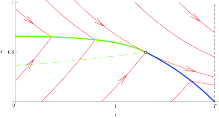
Figure 1: The field of trajectories of the ESS. Green solid line: the singular arc. Dotted green line: the singular arc of the cooperative solution.

Let a “resident” population “chooses” its behaviour, or strategy, $u$ in some strategy space $\mathcal{U}$, while a potential mutant —or cheater, or free-rider— would use a strategy $u_{m}\in\mathcal{U}$. Let $J(u,u_{m})$ and $J_{m}(u,u_{m})$ be the fitness of the resident and mutant population respectively under this scenario. By hypothesis, if the “mutant” behaves as the resident, there is no difference between them in terms of fitness, hence

$$J(u,u)=J_{m}(u,u)\,.$$ (20)

A strategy $u^{\star}\in\mathcal{U}$ is said to be uninvadable, or be a Wardrop equilibrium [17], if a  mutant cannot do better than a resident population using that strategy, i.e. if

$$\forall u_{m}\in\mathcal{U}\,,\quad J_{m}(u^{\star},u_{m})\leq J(u^{\star},u_{m})\,.$$

Let

$$\Delta J(u,v)=J_{m}(u,v)-J(u,v)\,.$$ (21)

Equivalently, the uninvadability property can be stated as

$$\sup_{u_{m}\in\mathcal{U}}\Delta J(u^{\star},u_{m})\leq 0\,.$$

However, it follows from (20) that $\Delta J(u^{\star},u^{\star})=0$, so that the supremum above is always non-negative. Hence, a strategy $u^{*}$ is uninvadable, or a Wardrop equilibrium, if and only if

$$\max_{u_{m}\in\mathcal{U}}\Delta J(u^{\star},u_{m})=\Delta J(u^{\star},u^{\star})=0\,.$$

And since this supremum is always non-negative, it follows that there exists a Wardrop equilibrium if and only if

$$\min_{u\in\mathcal{U}}\sup_{u_{m}\in\mathcal{U}}\Delta J(u,u_{m})=0\,.$$

Therefore, the search for a Wardrop equilibrium can be performed as follows : solve the zero-sum two-person game $\min_{u}\max_{u_{m}}\Delta J(u,u_{m})$, and if the min exists, check whether the min-sup reached yields a Value zero. If yes, the minimizing $u$ is a Wardrop equilibrium. If furthermore the maximum in $u_{m}$ is unique, then this is also an evolutionary stable strategy, or ESS [11, 10]. This is the case in the above problem.

4.2 Homogeneous problems

The following piece of theory can undoubtly be deduced from Noether’s theorem [14]. We offer a simple direct derivation. It accounts for the transformation we used via the introduction of the variable $x$.

4.2.1 The problem

Let a control problem be given by a state $y\in\mathbb{R}^{n}$, a control $u\in\mathsf{U}$, dynamics

$$\dot{y}=f(y,u),\quad y(0)=y_{0},$$

with all regularity and growth assumptions to guarantee existence of the solution for all measurable control functions $u(\cdot)\in\mathcal{M}(\mathbb{R}_{+}\to\mathsf{U})$.

A terminal condition $\mathcal{T}(y)=0$, $\mathcal{T}(\cdot)\in C^{1}(\mathbb{R}^{n})$, meaning that $t_{1}=\inf\{t\mid\mathcal{T}(y(t))=0\}$, and for simplicity we assume that all feasible trajectories are transverse to that differentiable manifold. A criterion to be minimized by the control action is given, of the form

$$J(y_{0},u(\cdot))=K(y(t_{1}))+\int_{0}^{t_{1}}\!L(y(t),u(t))\,\mathrm{d}t\,.$$

Assumptions

1. The functions $f$, $\mathcal{T}$, $K$ and $L$ are homogeneous of degree one in $y$.

2. The state variable $y_{n}$ remains strictly positive for all control functions.

It follows from these assumptions that if $\phi$ stands for $f$, $\mathcal{T}$, $K$ or $L$, and if $y^{(n-1)}$ stands for the first $n-1$ components of $y$, there exists a function of $n-1$ variables noted $\tilde{\phi}$ such that

$$\phi(y)=y_{n}\tilde{\phi}\left(\frac{1}{y_{n}}y^{(n-1)}\right)$$

Let also $x=(1/y_{n})y^{(n-1)}$. Then, we claim

Theorem

1. The reduced state $x(\cdot)$ obeys the dynamics

   $$\dot{x}=\tilde{g}(x,u)=\tilde{f}^{n-1}(x,u)-x\tilde{f}_{n}(x,u)\,,$$

2. The Value function $V(y)$ of this problem is homogeneous :

   $$V(y)=y_{n}U\left(\frac{1}{y_{n}}y^{(n-1)}\right)$$

3. The function $U$ solves the Hamilton Jacobi equation of the problem

   $$\tilde{J}(x_{0})=y_{n}(T)\widetilde{K}(y(T))+\int_{0}^{t_{1}}y_{n}(t)\tilde{L}(x(t),u(t))\,\mathrm{d}t\,.$$

   where

   $$y_{n}(t):=y_{n}(0)\exp\left(\int_{0}^{t}\tilde{f}_{n}(x(s),u(s))\,\mathrm{d}s\right).$$

4.2.2 Proof of the theorem

Dynamics

Direct calculations result in

$$\dot{x}_{i}=\frac{1}{y_{n}}f_{i}(y,u)-\frac{y_{i}}{y_{n}^{2}}f_{n}(y,u)=\tilde{g}_{i}(x,u)\,.$$

Value function

It is completely elementary to see that if the data are globally homogeneous of degree one in $x$, so is the Value function. Therefore, there exists $U$ such that $V(x)=x_{n}U((1/x_{n})x^{n-1}$.

Hamilton Jacobi equation

Easy calculations yield

$$\frac{\partial V}{\partial y_{i}}(y)=\frac{\partial U}{\partial x_{i}}(x),\>i=1,\ldots,n-1,$$

and

$$\frac{\partial V}{\partial y_{n}}(y)=U(x)-\sum_{i=1}^{n-1}x_{i}\frac{\partial U}{\partial x_{i}}(x).$$

Substitute these in the standard Hamilton Jacobi equation

$$\max_{u}\left[\frac{\partial V}{\partial y}f(y,u)+L(y,u)\right]=0\,,$$

to get (with $x:=(1/y_{n})y^{(n-1)}$)

$$\max_{u}\left[\frac{\partial U}{\partial x}(x)f^{n-1}(y,u)+f_{n}(y,u)\left(U(x)-\frac{\partial U}{\partial x}(x)x\right)+L(y,u)\right]=0\,.$$

If $y_{n}\neq 0$, we may write this as

$$\max_{u}y_{n}\left[\tilde{f}_{n}(x,u)U(x)+\frac{\partial U}{\partial x}(x)\tilde{g}(x,u)+\tilde{L}(x,u)\right]=0\,.$$

If furthermore $y_{n}(t)>0$, then we may divide through by $y_{n}$ without changing the $\max$ operator. We recognize the Hamilton Jacobi Bellman equation of the problem with an exponential discount factor $\exp\int\tilde{f}_{n}(x,u)$. However, multiplied by the positive constant $y_{n}(0)$, this exponential is indeed $y_{n}(t)$.

The terminal condition $\mathcal{T}(y)=0$ translates into $\widetilde{\mathcal{T}}(x)=0$, and the boundary condition of the H.J.B. equation into $\forall x:\widetilde{\mathcal{T}}(x)=0$, $U(x)=\widetilde{K}(x)$.

4.3 Mixed strategy vs mixed population

We want to investigate here the possible meanings of the mixed, singular strategy. Recall that in our model, $u=0$ means reproducing, while $u=1$ means feeding. What is the meaning of an intermediary strategy $u\in(0,1)$ ?

One possible interpretation is that each individual in the population spends some time eating and some time reproducing in a fast cycle, as compared to the horizon of the problem —here a year— and to the characteristic frequency of the dynamics, here $a$ and $c$. This thus a monomorphic population agreeing on a mixed strategy for all individuals.

In linear problems, it is possible to think of an intermediary $\tilde{u}$ as representing a polymorphic population, where a fraction $\tilde{u}$ uses the strategy $u=1$ while a fraction $1-\tilde{u}$ uses the strategy $u=0$. However, our criterion here is nonlinear. Therefore further investigation is needed.

Let the population be represented by a measured space $\Omega$, with a positive measure $\mu$ of total mass $\mu(\Omega)=1$. (It is thus a probability measure.) Each individual is represented as an $\omega\in\Omega$. Assume also that each individual $\omega$ has to pick, at each instant of time, a control $v(\omega,t)\in\{0,1\}$. We need to assume that $\omega\mapsto v(\omega,t)$ is $\mu$-measurable for (allmost) all $t\in[0,T]$, and that, for (allmost) all $\omega\in\Omega$, $t\mapsto v(\omega,t)$ is piecewise constant, equal to $0$ or $1$ on time intervals (hence Lebesgue measurable).

Each individual has an energy $\pi(\omega,t)$ at time $t$. Its dynamics are

$$\dot{\pi}(\omega,t)=-a\pi(\omega,t)+bn(t)v(\omega,t)\,.$$

The rsource depletion rate is

$$\dot{n}=-cn\int_{\Omega}\!v(\omega,t)\,\mathrm{d}\mu(\omega)\,.$$

So, if we set

$$u(t)=\int_{\Omega}\!v(\omega,t)\,\mathrm{d}\mu(\omega)=\mu(\{\omega\mid v(\omega,t)=1\})$$

and

$$p(t)=\int_{\Omega}\!\pi(\omega,t)\,\mathrm{d}\mu(\omega)\,,$$

we find equations (1) and (2), as it should.

The number of offspring produced by an individual is

$$f(\omega)=\int_{0}^{T}\!(1-v(\omega,t))\pi(\omega,t)\,\mathrm{d}t\,,$$

and for the whole population (using Fubini’s theorem)

$$F=\int_{\Omega}\!f(\omega)\,\mathrm{d}\mu(\omega)=\int_{0}^{T}\!\left[\int_{\Omega}(1-v(\omega,t))\pi(\omega,t)\,\mathrm{d}\mu(\omega)\right]\mathrm{d}t$$

which would coincide with the formula (4) for $J$ only if $\pi(\omega,t)$ and $v(\omega,t)$ were probabilistically independant, an impossible situation if each player uses a constant control on nonzero, measurable, time intervals. We would approach such an independance if we were to assume that the time intervals during which the individuals’controls are constant are extremely short, and after each, the set of individuals using $u=1$, say, is drawn at random, with probability $u(t)$, independantly of $\pi(\omega,t)$. But this is reconstructing a monomorphic population of mixed players.

Appendix A Switch function on feeding tributaries

A.1 All tributaries with $u=1$

Let $t_{s}$, $x_{s}$, $\lambda_{s}$, $\mu_{s}$ stand for the variables $t$, $x$, $\lambda$ and $\mu$ at the point where a trajectory with $u=1$ meets either the switch line or a singular arc, either cooperative or uninvadable. To simplify the notations, let also

$$\alpha:=\mathrm{e}^{-a(t_{s}-t)}\,,\qquad\gamma:=\mathrm{e}^{-c(t_{s}-t)}\,.$$

On this trajectory, we have

$$x(t) = \left(x_{s}+\frac{b}{c-a}\right)\alpha-\frac{b}{c-a}\,,$$

$$\lambda(t) = \lambda_{s}\alpha\,,$$

$$\mu(t) = \mu_{s}\gamma+\frac{b}{c-a}(\alpha-\gamma)$$

We want to investigate the sign of

$$\sigma=b\lambda-c\mu-x\,,$$

remembering that in all cases to be investigated, $\sigma(t_{s})=0$. We have already noticed that

$$\dot{\sigma}=c\sigma+ab\lambda+ax-b\,.$$

Hence

$$\sigma=-\int_{t}^{t_{s}}\mathrm{e}^{-c(\tau-t)}(ab\lambda(\tau)+ax(\tau)-b)\,\mathrm{d}\tau\,.$$ (22)

We wish to show that $L(\tau):=ab\lambda(\tau)+ax(\tau)-b<0$, thus proving that $\sigma$ is positive from $t=0$ to $t_{s}$. Substituting the explicit values of $x$, $\lambda$ and $\mu$, we get

$$L(t)=a\left[b\lambda_{s}\alpha+x_{s}\frac{\gamma}{\alpha}+\frac{b}{c-a}\left(\frac{\gamma}{\alpha}-\frac{c}{a}\right)\right]$$

A.2 Tributaries of the switch line

On the switch line, $x_{s}=b\lambda_{s}$ and $\mu_{s}=0$. Hence

$$L=ab\left[\lambda_{s}\left(\alpha+\frac{\gamma}{\alpha}\right)+\frac{1}{c-a}\left(\frac{\gamma}{\alpha}-\frac{c}{a}\right)\right]$$

We notice that $L(t_{s})=ab(2\lambda_{s}-1/a)$. But we know that on the switch line $\lambda_{s}\leq 1/2a$. Hence $L(t_{s})\leq 0$. Let us investigate its time derivative:

$$\frac{1}{ab}\dot{L}(t)=\lambda_{s}\left(a\alpha+(c-a)\frac{\gamma}{\alpha}\right)+\frac{\gamma}{\alpha}=a\lambda_{s}\alpha+\left((c-a)\lambda_{s}+1\right)\frac{\gamma}{\alpha}\,.$$

Hence $\frac{1}{ab}\dot{L}>(-a\lambda_{s}+1)\gamma/\alpha>0$, and therefore, $L(t)\leq 0$ for allt $t\leq t_{s}$.

A.3 Tributaries of the singular arcs

We now have

$$L(t_{s})=a(b\lambda_{s}+x_{s})-b\,.$$

We claim that $x_{s}<b/a$. As a matter of fact, on the singular arc of the cooperative solution, $x_{s}\leq b/2a$. On the singular arc of the uninvadable solution,

$$x_{s}\leq\bar{x}=\frac{b}{2a}\left[1+\frac{\sqrt{4a^{2}+c^{2}}-2a}{c}\right]\,.$$

It is easy to chack that $\sqrt{4a^{2}+c^{2}}-2a<c$, so that indeed, $x_{s}<b/a$, and therefore, $L(t_{s})<0$. Again, compute its time derivative:

$$\dot{L}(t)=a\left[ab\lambda_{s}\alpha+\left((c-a)x_{s}+b\right)\frac{\gamma}{\alpha}\right]>0$$

again thanks to $b-ax_{s}>0$. So, again, we may conclude that for all $t\leq t_{s}$, $L(t)<0$.

In all three cases, we conclude with the help of formula (22) that on these trajectories, for all $t\leq t_{s}$, $\sigma(t)>0$.

Acknowledgement

This work is supported by Agropolis Foundation and the Réseau National des Systèmes Complexes (RNSC) under the ModPEA Project.

References

- [1] Akhmetzhanov, A. R., Grognard, F. and Mailleret, L. Optimal life-history strategies in a seasonal consumer-resource model In preparation. 2010.
- [2] Akhmetzhanov, A. R., Grognard, F., Mailleret, L. and Bernhard, P. Join forces or cheat: evolutionary analysis of a consumer-resource system. in Proceedings of the 14th International Symposium on Dynamic Games and Applications. Banff, Canada, 2010.
- [3] Dercole, F. and Rinaldi, S. Analysis of evolutionary processes: the Adaptive Dynamics approach and its applications. Princeton University Press, 2008.
- [4] Eskola, H. T. M. On the evolution of the timing of reproduction. Theoretical Population Biology 75, pp. 98–108, 2009.
- [5] Geritz, S. A. H., Metz, J. A. J., Kisdi, E. and Meszena, G. Dynamics of adaptation and evolutionary branching. Physical Review Letters 78 (10), pp. 2024–2027, Â 1997.
- [6] Heino, M. and Kaitala, V. Evolution of resource allocation between growth and reproduction in animals with indeterminate growth. Journal of Evolutionary Biology 12, pp. 423–429, 1999.
- [7] Iwasa, Y. Dynamic optimization of plant growth. Evolutionary Ecology Research 2, pp. 437–455, 2000.
- [8] Lessells, C. M. The evolution of life histories. In: Krebs, J. R., Davies, N. B. (Eds.), Behavioural Ecology. Blackwell Scientific Publications, pp. 32–68, 1991.
- [9] Mailleret, L. and Lemesle, V. A note on semi-discrete modelling in the life sciences. Philosophical Transactions of the Royal Society, A. 367, pp. 4779-4799, 2009.
- [10] Maynard Smith, J. Evolution and the Theory of Games. Cambridge University Press, Cambridge, U.K., 1982.
- [11] Maynard Smith, J. and  Price, G. R. The logic of animal conflict. Nature, 246, pp. 15–18, 1973.
- [12] Metz, J. A. J., Mylius, S. D., and Diekmann, O. When does evolution optimize ? Evolutionary Ecology Research 10, pp. 629–654, 2008.
- [13] Mylius, S. D. and Diekmann, O. On evolutionarily stable life histories, optimization and the need to be specific about density dependence. Oikos 74, pp. 218–224, 1995.
- [14] Noether, E. Invariante Variationsprobleme. Nachrichten der Königlichen Gesellschaft der Wissenschaften zu Göttingen. Math.-phys. Klasse, pp. 235-257, 1918.
- [15] Perrin, N. and Sibly, R. M. Dynamic-models of energy allocation and investment. Annual Review of Ecology and Systematics 24, pp. 379–410, 1993.
- [16] Stearns, S. The Evolution of Life Histories. Oxford University Press, 1992.
- [17] Wardrop, J. G. Some theoretical aspects of road traffic research. Proceedings of the Institution of Civil Engineers, pp. 325–378, 1952.