Asymptotic-preserving projective integration schemes for kinetic equations in the diffusion limit

Abstract

We investigate a projective integration scheme for a kinetic equation in the limit of vanishing mean free path, in which the kinetic description approaches a diffusion phenomenon. The scheme first takes a few small steps with a simple, explicit method, such as a spatial centered flux/forward Euler time integration, and subsequently projects the results forward in time over a large time step on the diffusion time scale. We show that, with an appropriate choice of the inner step size, the time-step restriction on the outer time step is similar to the stability condition for the diffusion equation, whereas the required number of inner steps does not depend on the mean free path. We also provide a consistency result. The presented method is asymptotic-preserving, in the sense that the method converges to a standard finite volume scheme for the diffusion equation in the limit of vanishing mean free path. The analysis is illustrated with numerical results, and we present an application to the Su-Olson test.

1 Introduction

In many applications, ranging from radiative transfer over rarefied gas dynamics to cell motion in biology, the underlying physical system consists of a large number of moving and colliding particles. Such systems can be accurately modelled using a kinetic mesoscopic description that governs the evolution of the particle distribution in position-velocity phase space. In a diffusive scaling, when the mean free path of the particles is small with respect to the (macroscopic) length scale of interest, a macroscopic description involving only a few low-order moments of the particle distribution (such as a diffusion equation in neutron transport and radiative transfer, or fluid equations in rarefied gas dynamics) may give a rough idea of the behavior. However, refining the description is uneasy because, whereas the physical model becomes much simpler in the diffusion limit, a direct numerical simulation of the kinetic model tends to be prohibitively expensive due to the additional dimensions in velocity space and stability restrictions that depend singularly on the mean free path.

We consider dimensionless kinetic equations of the type

$$\partial_{t}f_{\epsilon}+\frac{v}{\epsilon}\cdot\nabla_{x}f_{\epsilon}=\frac{1}{\epsilon^{2}}Q(f_{\epsilon}),$$ (1.1)

modeling the evolution of a particle distribution function $f_{\epsilon}(x,v,t)$ that gives the distribution density of particles at a given position $x\in U\subset\mathbb{R}^{d}$ with velocity $v\in V\subset\mathbb{R}^{d}$, $d\geq 1$, at time $t$, the collisions being embodied in the operator $Q$. The parameter $\epsilon>0$ is meant as the ratio of the mean free path over the characteristic length of observation, i.e. the average distance traveled by the particles between collisions. The diffusion limit is obtained by taking $\epsilon\to 0$. Under some appropriate assumptions, which will be detailed in section 2, the unknown $f_{\epsilon}$ then relaxes on short time-scales to an equilibrium, in which the dependence on $v$ is fixed, and the dynamics of the system on long time-scales can be described as a function of the density $\rho_{\epsilon}(x,t)=\langle f_{\epsilon}(x,v,t)\rangle$, where

$$\langle\cdot\rangle=\int_{V}\;\cdot\;d\mu(v),$$

is the averaging operator over velocity space and $(V,d\mu)$ denotes the measured velocity space. For $\epsilon\to 0$, the density $\rho=\lim_{\epsilon\to 0}\rho_{\epsilon}$ satisfies formally the diffusion equation

$$\partial_{t}\rho-d\Delta_{x}\rho=0,\qquad d_{p}=\langle v^{2}\rangle.$$ (1.2)

The difficulty in studying the asymptotic behavior numerically is precisely due to the presence of two time-scales. On the one hand, explicit time integration of equation (1.1) is numerically challenging because one is forced to take very small time-steps $\delta t$ when $\epsilon\to 0$ to stably integrate the fast relaxation. Indeed, due to stability considerations, $\delta t$ needs to be shrunk as $\epsilon\to 0$ to properly satisfy both the $\epsilon$-dependent hyperbolic Courant-Friedrichs-Lewy (CFL) condition for equation (1.1) and the stability constraints for the collision term. On the other hand, implicit schemes are computationally expensive because of the extra dimensions in velocity space. At the same time, the equation closely resembles a diffusion equation in that limit, for which a parabolic CFL condition of the type $\Delta t=O(\Delta x^{2})$ (independently of $\epsilon$) would be desirable.

A number of specialized methods that are asymptotic-preserving in the sense introduced by Jin [11] have been developed that can integrate equation (1.1) in the limit of $\epsilon\to 0$ with time-steps that are only limited by the stability constraints of the diffusion limit. We briefly review here some efforts, and refer to the cited references for more details. In [13, 16], separating the distribution $f$ into its odd and even parts in the velocity variable results in a coupled system of transport equations where the stiffness appears only in the source term, allowing to use a time-splitting technique [24] with implicit treatment of the source term; see also related work in [11, 12, 17, 18, 22]. When the collision operator allows for an explicit computation, an explicit scheme can be obtained by splitting $f$ into its mean value and the first-order fluctuations in a Hilbert expansion form [9] under a classical diffusion CFL. Also, closure by moments [5, 21, e.g.] can lead to reduced systems for which time-splitting provides new classes of schemes [4]. Alternatively, a micro-macro decomposition based on a Chapman-Enskog expansion has been proposed [20], leading to a system of transport equations that allows to design a semi-implicit scheme without time splitting. An innovative non-local procedure based on the quadrature of kernels obtained through pseudo-differential calculus was proposed in [2].

Our goal is to introduce a different point of view, based on methods that were developed for large multiscale systems of ODEs. In [8], projective integration methods were introduced as a class of explicit methods for the solution of stiff systems of ordinary differential equations (ODEs) that have a large gap between their fast and slow time scales; these methods fit within recent efforts to systematically explore numerical methods for multiscale simulation [6, 7, 14, 15]. In projective integration, the fast modes, that correspond to the Jacobian eigenvalues with large negative real parts, decay quickly, whereas the slow modes correspond to eigenvalues of smaller magnitude and are the solution components of practical interest. Such problems are called stiff, and a standard explicit method requires time steps that are very small compared to the slow time scales, just to ensure a stable integration of the fast modes. Projective integration circumvents this problem. The method first takes a few small (inner) steps with a simple, explicit method, until the transients corresponding to the fast modes have died out, and subsequently projects (extrapolates) the solution forward in time over a large (outer) time step; a schematic representation of the scheme is given in figure 1.

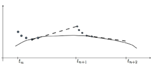
Figure 1: Schematic representation of projective forward Euler. In a stiff system with a spectral gap, the values of the solution obtained by straightforward explicit integration (dots) are quickly attracted to a slow manifold (solid curve). Projective integration takes a few explicit inner steps until the solution has come down to this slow manifold. Then, a chord slope estimation is performed, and a big projective outer step is taken. Since the result of the outer step does not lie on the slow manifold, a number of inner steps is taken again, and the procedure is repeated.

A stability analysis in the ODE setting was presented for a first order version, called projective forward Euler [8], and an accuracy analysis was given in [26]. Higher-order versions have been proposed in [19, 23].

Projective integration methods can offer a number of important advantages for the simulation of kinetic equations. In particular, they are fully explicit and do not require any splitting, neither in time, nor in microscopic and macroscopic variables. In this work, we will analyze the properties of projective integration for kinetic equations on diffusive time scales in one space dimension, keeping in mind that these methods extend readily to higher dimensions. The paper is organized as follows. In section 2, we give the necessary preliminaries on the model problem (1.1) and present its diffusion asymptotics. We also introduce the Su-Olson test case that will be used in the numerical experiments. In section 3, we develop the numerical scheme. We present the brute-force inner schemes and the projective outer forward Euler method. In section 4, we show that, when choosing the inner time step $\delta t=\epsilon^{2}$, the stability condition on the outer time step is independent of $\epsilon$, and similar to the CFL condition of the limiting heat equation. Moreover, the required number of inner steps is also independent of $\epsilon$ when $\epsilon\to 0$. Subsequently, in section 5, we study the consistency of the method and, using the stability condition derived in section 4, we give a bound of the convergence error, enabling to conclude that the presented scheme is asymptotic-preserving. We provide numerical illustrations for the linear model and the Su-Olson test in section 6. Finally, section 7 contains conclusions and an outlook to future work.

2 Model problem and diffusion asymptotics

2.1 Linear relaxation

We consider equation (1.1) in one space dimension,

$$\partial_{t}f_{\epsilon}+\dfrac{v}{\epsilon}\partial_{x}f_{\epsilon}=\dfrac{1}{\epsilon^{2}}Q(f_{\epsilon}),$$ (2.1)

and specify the collision operator as a linear relaxation

$$Q(f_{\epsilon})=\langle f_{\epsilon}\rangle-f_{\epsilon}=\rho_{\epsilon}-f_{\epsilon}$$

that can be interpreted as the difference of a gain and a loss term. In the remainder of the text, we restrict the discussion to a periodic setting in one space dimension, hence $x\in\mathbb{T}=[0,1)$ and $v\in V\subset\mathbb{R}$. The results of the derivation, however, could easily be generalized to higher space dimensions.

Throughout the paper, the measured velocity space $(V,\mu)$ is required to satisfy

$$\begin{cases}\int_{V}d\mu(v)=1,\\ \int_{V}h(v)d\mu(v)=0,\qquad\text{for any odd integrable function $h:V\longrightarrow\mathbb{R}$,}\\ \int_{V}v^{2}d\mu(v)=d>0.\end{cases}$$

Typical examples are

• $V=(-1,1)$ endowed with the normalized Lebesgue measure, for which we have $d=1/3$;

• the discrete velocity space

  $$V=\{-v_{p},\ldots,-v_{1},v_{1},\ldots,v_{p}\},\text{ with }v_{j}=\dfrac{2j-1}{2p},\,\,j\in\mathcal{J}=\mathcal{J}_{+}\cup\mathcal{J}_{-},$$ (2.2)

  where $\mathcal{J}_{\pm}:=\{\pm 1,\ldots,\pm p\}$, endowed with the normalized discrete velocity measure $d\mu(v)=\dfrac{1}{2p}\sum_{j\in\mathcal{J}}\delta(v-v_{j})$, for which

  $$d_{p}=\dfrac{\sum_{j}v_{j}^{2}}{2p}=\dfrac{4p^{2}-1}{12p^{2}}$$

  so that $d_{p}\to 1/3$ as $p\to\infty$;

• $V=\mathbb{R}$ endowed with the Gaussian measure $d\mu(v)=(2\pi)^{-1/2}\exp(-v^{2}/2)dv$, for which $d=1$.

These assumptions on the velocity space result in a number of properties for $Q$, namely :

1. $Q$ is a bounded operator on $L^{p}(V,d\mu(v)),1\leq p\leq\infty$;

2. $Q$ is conservative, i.e.

   $$\forall f\in L^{1}(V,d\mu(v)):\langle Q(f)\rangle=0;$$

3. the elements of the kernel of $Q$ are independent of $v$.

As $\epsilon\to 0$, the frequency of collisions increases; hence, we may formally propose to write $f_{\epsilon}$ as a perturbation of the macroscopic density $\rho_{\epsilon}=\langle f_{\epsilon}\rangle$ using a Hilbert expansion:

$$f_{\epsilon}(x,v,t)=\rho_{\epsilon}(x,t)+\epsilon g_{\epsilon}(x,v,t).$$ (2.3)

Equation (2.1) can then alternatively be written as

$$\begin{cases}\partial_{t}\rho_{\epsilon}(x,t)+\langle v\partial_{x}g_{\epsilon}(x,v,t)\rangle=0,\\ \partial_{t}g_{\epsilon}(x,v,t)+\dfrac{1}{\epsilon}\left(v\partial_{x}g_{\epsilon}-\langle v\partial_{x}g_{\epsilon}\rangle\right)=-\dfrac{1}{\epsilon^{2}}\left(g_{\epsilon}+v\partial_{x}\rho_{\epsilon}\right).\end{cases}$$ (2.4)

Taking formally the limit $\epsilon\to 0$ yields

$$\partial_{t}\rho_{\epsilon}-\langle v^{2}\rangle\partial_{xx}\rho_{\epsilon}=O(\epsilon^{2}),$$ (2.5)

since

$$g_{\epsilon}=-v\partial_{x}\rho_{\epsilon}+\epsilon\left\{\langle v\partial_{x}g_{\epsilon}\rangle-v\partial_{x}g_{\epsilon}\right\}+O(\epsilon^{2}).$$ (2.6)

The approximation (2.5) is consistent at order 2 in $\epsilon$ with the diffusion equation (1.2). We refer to [5] for a recent starting point of the literature on the convergence of $f_{\epsilon}$ to $\rho$, solution of (1.2).

For concreteness, we will use the discrete velocity space (2.2) in our analysis and simulations. Thus, we are now interested in a vector-valued function $f_{\epsilon}:\mathbb{R}^{+}\times\mathbb{T}\longrightarrow\mathbb{R}^{2p}$, of which we denote the component corresponding to $v_{j}$ as $f_{\epsilon,j}(t,x)$, $\forall j\in\mathcal{J}$. In this setting, the density is given as $\rho_{\epsilon}=\left(\sum_{j}f_{\epsilon,j}\right)/(2p)$. The kinetic equation (2.1) then reads

$$\forall j\in\mathcal{J},\qquad\partial_{t}f_{\epsilon,j}+\frac{v_{j}}{\epsilon}\partial_{x}f_{\epsilon,j}=\frac{\rho_{\epsilon}-f_{\epsilon,j}}{\epsilon^{2}}.$$ (2.7)

2.2 Su-Olson equation

While the linear kinetic equation (2.1) is an ideal model problem for analysis purposes, we will also show numerical results for a more challenging test case, namely the traditional Su-Olson benchmark, a prototype model for radiative transfer problems. Here, the unknown $f_{\epsilon}$ represents the specific intensity of radiations, which interact with matter through energy exchanges; see e.g. [2, 3, 4, 25]. A complete model couples a kinetic equation for the evolution of $f_{\epsilon}$ with the Euler system describing the evolution of the matter. In the Su-Olson test, this coupling is replaced by a simple ODE describing the evolution of the material temperature. The system reads

$$\begin{cases}&\partial_{t}f_{\epsilon}+\dfrac{v}{\epsilon}f_{\epsilon}=\dfrac{1}{\epsilon^{2}}\left(\rho_{\epsilon}-f_{\epsilon}\right)+\sigma_{a}\left(\Theta-\rho_{\epsilon}\right)+S,\\ &\partial_{t}\Theta=\sigma_{a}\left(\rho_{\epsilon}-\Theta\right).\end{cases}$$ (2.8)

Here, $\Theta=T^{4}$, with $T$ the material temperature, and $S$ is a given source depending on $x$. In our simulations, the parameter $\sigma_{a}=1$.

3 Numerical scheme

3.1 Finite volume formulation

We consider a uniform, constant in time, periodic spatial mesh with spacing $\Delta x$, consisting of cells $C_{i}=[x_{i-1/2},x_{i+1/2})$, $1\leq i\leq N_{x}$ with $N_{x}\Delta x=1$ centered in $x_{i}$, where $x_{i}=i\Delta x$, and a uniform mesh in time $T_{k}=[t^{k},t^{k+1})$, $k\geq 0$, $t^{k}=k\delta t$ where $\delta t$ is the time step. We adopt a finite volume approach, that is we integrate (2.7) on a cell $M_{i,k}=C_{i}\times T_{k}$ to obtain, $\forall j\in\mathcal{J}$,

$$\int_{C_{i}}(f_{\epsilon,j}(t^{k+1},\cdot)-f_{\epsilon,j}(t^{k},\cdot))+\dfrac{v_{j}}{\epsilon}\left(\int_{T_{k}}(f_{\epsilon,j}(\cdot,x_{i+1/2})-f_{\epsilon,j}(\cdot,x_{i-1/2}))\right)=\dfrac{1}{\epsilon^{2}}\int_{M_{i,k}}\left(\rho_{\epsilon}-f_{\epsilon,j}\right).$$

In order to simplify the notations, the solution of the continuous equation (2.7) $f_{\epsilon}$ will always be denoted with the subscript $\epsilon$ whereas the solution of the numerical scheme will be denoted $f=(f^{k}_{i,j})$. This leads to the conservative forward Euler scheme

$$f_{i,j}^{k+1} =f_{i,j}^{k}-\dfrac{\delta t}{\epsilon\Delta x}\left(\phi(f)_{i+1/2,j}^{k}-\phi(f)_{i-1/2,j}^{k}\right)+\dfrac{\delta t}{\epsilon^{2}}\left(\rho^{k}_{i}-f^{k}_{i,j}\right),$$ (3.1)

where $f_{i,j}^{k}$ denotes an approximation of the mean value $\int_{C_{i}}f_{\epsilon,j}(t^{k},x)\mathrm{d}x$, the numerical flux $\phi(f)_{i+1/2,j}^{k}$ is an approximation of the flux at the interface $x_{i+1/2}$ at time $t^{k}$ in the equation for the velocity $j$, and $\rho^{k}_{i}=\langle f_{i}^{k}\rangle$, the average being taken over the velocity index. We will consider upwind or centered numerical fluxes that are given by

$$\phi_{u}(f)^{k}_{i+1/2,j}=\begin{cases}v_{j}f^{k}_{i,j},&\text{ if }j\in\mathcal{J}_{+}\;\;(v_{j}>0),\\ v_{j}f^{k}_{i+1,j},&\text{ if }j\in\mathcal{J}_{-}\;\;(v_{j}<0),\end{cases}$$ (3.2)

$$\phi_{c}(f)^{k}_{i+1/2,j}=v_{j}\dfrac{f^{k}_{i+1,j}+f^{k}_{i,j}}{2},$$ (3.3)

respectively. We introduce a generic short-hand notation,

$$f^{k+1}=S_{\delta t}f^{k},$$ (3.4)

with $f\in\mathbb{R}^{N_{x}\times 2p}$ and $S_{\delta t}$ a square matrix of order $N_{x}\times 2p$.

Remark 3.1 (Maximum principle).

We recall that, while the centered flux scheme (3.3) is second-order accurate in space, it does not obey a maximum principle, and hence may lead to unphysical oscillations, the centered transport scheme being violently unstable for transport equations. Any projective integration scheme based on the centered flux scheme should therefore also violate the maximum principle. However, since the kinetic equation (2.1) is consistent at order 2 in $\epsilon$ with a diffusion equation (2.5), the oscillations are quickly stabilized as $\epsilon\to 0$ (see also the discussion on consistency in section 5).

3.2 Projective integration

Because of the presence of the small parameter $\epsilon$, the time steps that one can take with the upwind scheme are at most $O(\epsilon)$, due to the CFL stability condition for the transport equation, or $O(\epsilon^{2})$ due to the relaxation term. However, in the diffusion limit, as $\epsilon$ goes to $0$, the equation tends to the diffusion equation (1.2), for which a standard finite volume/forward Euler method only needs to satisfy a stability restriction of the form $\Delta t\leq\Delta x^{2}/(2d)$.

In this paper, we consider the use of projective integration [8] to accelerate brute force integration; the idea is the following (see also figure 1). Starting from an approximate solution $f^{N}$ at time $t^{N}=N\Delta t$, one first takes $K+1$ inner steps of size $\delta t$,

$$f^{N,k+1}=S_{\delta t}f^{N,k},\qquad k=0,\ldots,K,$$

in which the superscript pair $(N,k)$ represents an approximation to the solution at $t^{N,k}=N\Delta t+k\delta t$. The aim is to obtain a discrete derivative to be used in the outer step to compute $f^{N+1}=f^{N+1,0}$ via extrapolation in time, e.g.,

$$f^{N+1}=f^{N,K+1}+\left(\Delta t-(K+1)\delta t\right)\frac{f^{N,K+1}-f^{N,K}}{\delta t}.$$ (3.5)

This method is called projective forward Euler, and it is the simplest instantiation of this class of integration methods [8]. Adams–Bashforth or Runge–Kutta extensions of (3.5), giving a higher order consistency in terms of $\Delta t$, are possible [19, 23].

Projective integration is a viable asymptotic-preserving scheme if, as $\epsilon$ goes to $0$, we have (i) a stability for the outer time step $\Delta t$ that should satisfy a condition similar to the CFL condition for the diffusion equation, (ii) a number of inner steps that is independent of $\epsilon$ and (iii) the consistency with the diffusion equation (1.2). The analysis of these properties will be performed in the next sections.

4 Stability analysis

4.1 Notations

To perform a Von Neumann analysis of the projective forward Euler scheme, we need the following notations :

• $e:=\dfrac{1}{\sqrt{2p}}(1,\ldots,1)^{T}\in\mathbb{R}^{2p}$ and $\mathcal{P}:=ee^{T}$ is the orthogonal projection on $\mbox{Span}(e)$;

• $\forall W\in\mathbb{R}^{2p}$, $\mathcal{P}W=\langle W\rangle(1,\ldots,1)^{T}=\sqrt{2p}\langle W\rangle e$, with $\displaystyle\langle W\rangle=\dfrac{1}{2p}\sum_{j=1}^{2p}x_{j}$,

• for all $\zeta=\xi\Delta x$, $\xi\in\mathbb{R}$, $\mathcal{V}_{C}(\zeta):=\dfrac{\sin(\zeta)}{\Delta x}\,\mathrm{diag}(v_{p},\ldots,v_{1},-v_{1},\ldots,-v_{p})$ and

  $\mathcal{V}_{U}(\zeta):=\dfrac{2\sin(\zeta/2)}{\Delta x}\,\mathrm{diag}(v_{p}e^{i\zeta/2},\ldots,v_{1}e^{i\zeta/2},-v_{1}e^{-i\zeta/2},\ldots,-v_{p}e^{-i\zeta/2})$.

We also introduce the symbol $\mathcal{D}\left(\alpha,\beta\right)$ to denote a closed disk with center $\alpha$ and radius $\beta$.

4.2 Forward Euler schemes

Let us first locate the spectrum of the matrix $S_{\delta t}$ defined in (3.4). We denote $h=S_{\delta t}f$ and compute the Fourier series in space of periodized reconstructions of $f$ and $h$ as constant-by-cell functions $F:x\mapsto f_{i}\mbox{ if }x\in C_{i}$ and $H:x\mapsto h_{i}\mbox{ if }x\in C_{i}$ : $\forall m\in\mathbb{Z}$,

$$\hat{H}(m)=\mathcal{A}\hat{F}(m)=\left(\left(1-\dfrac{\delta t}{\epsilon^{2}}\right)I_{2p}+\dfrac{\delta t}{\epsilon}i\mathcal{V}+\delta t\dfrac{\mathcal{P}}{\epsilon^{2}}\right)\hat{F}(m)$$ (4.1)

where $\hat{F}(m):=\int_{0}^{1}e^{-im2\pi x}f(x)\mathrm{d}x$, and correspondingly $\hat{H}(m)$, are the $m$-th Fourier coefficients of $F$ and $H$ and $\mathcal{V}$ is the (diagonal) Fourier matrix of the finite volume operator chosen for the convection part. We will give hereafter the results for $\mathcal{V}=\mathcal{V}_{C}$ and $\mathcal{V}=\mathcal{V}_{U}$. Since $F\in L^{2}(0,1)\mapsto(\hat{F}(m))_{m}\in\ell^{2}(\mathbb{Z})$ is an isometry, studying the stability of the scheme is equivalent to studying the spectrum of $\mathcal{A}$.

We first prove an auxiliary result. For the sake of simplicity, the matrix $\mathcal{V}$ being a diagonal complex matrix, we can study the spectrum of a typical matrix $A=D+P$ where $P=(1,\ldots,1)^{T}(1,\ldots,1)$ and $D$ is a diagonal matrix with complex entries.

Proposition 4.1.

Let $D=\,\mathrm{diag}(D_{1},\ldots,D_{2p})$, with $D_{j}\in\mathbb{C}$. Then the following properties of $A=D+P$ hold :

• if $D_{j}=D_{k}$ implies $j=k$ (H1), the eigenspaces of $A$ are all of dimension 1 and the spectrum of $A$ does not contain any $D_{k}$ ;

• if moreover we assume that $\overline{D_{j}}=D_{2p-j+1}$ $\forall j\in\mathcal{J}_{+}$ (H2), then an eigenvalue of $A$ is

  • either real

  • or complex-conjugate and lies in one of the disks of diameters $[D_{j},\overline{D_{j}}],\,j\in\mathcal{J}_{+}$ (see figure 2.a);

    (a) (P2)

    (b) (P3)

    Figure 2: Spectrum of $A$ in case (P2) and in case (P3) where $\mathcal{D}_{\epsilon}=\mathcal{D}\left(0,\epsilon\max_{j\in\mathcal{J}^{+}}(|\alpha_{j}|+|\beta_{j}|)\right)$.+

• if, in addition to the previous hypotheses, $D$ is of order $\epsilon$, $\epsilon$ being small, that is $D=\epsilon\,\mathrm{diag}(\alpha_{p}-i\beta_{p},\ldots,\alpha_{1}-i\beta_{1},\alpha_{1}+i\beta_{1},\ldots,\alpha_{p}+i\beta_{p})$ (H3), then

  $$\mbox{\emph{Sp($A$)}}\subset\left(\mathcal{D}\left(0,\epsilon\max_{j\in\mathcal{J}^{+}}(|\alpha_{j}|+|\beta_{j}|)\right)\setminus\mathbb{R}\right)\cup\{\lambda(\epsilon)\}$$

  where the only real eigenvalue $\lambda(\epsilon)$ is simple and can be expanded as

  $$\lambda(\epsilon)=2p\left(1+\epsilon\dfrac{\langle\alpha\rangle}{2p}-\dfrac{\epsilon^{2}}{4p^{2}}\langle(\alpha-\langle\alpha\rangle)^{2}+\beta^{2}\rangle\right)+o(\epsilon^{2}),$$

  (see figure 2.b).

Proof.

Assume (H1). Let $(\lambda,W)$ be an eigenvalue and an associated eigenvector. Then $(D+P)W=\lambda W\Longleftrightarrow(\lambda I_{2p}-D)W=\sqrt{2p}\langle W\rangle e$. There are two possibilities :

• either $\langle W\rangle=0$ and there exists a pair of indices $(k_{1},k_{2})\in\{1,\ldots,2p\},k_{1}\neq k_{2}$ such that $x_{k_{1}}\neq 0$ and $x_{k_{2}}\neq 0$, which implies that $\lambda=D_{k_{1}}=D_{k_{2}}$, which is incompatible with (H1) ;

• or $\langle W\rangle\neq 0$ and $W=\sqrt{2p}\langle W\rangle(\lambda I_{2p}-D)^{-1}e$, that is, the eigenspaces of $A$ are all of dimension 1 and no $D_{k}$ can be an eigenvalue of $A$.

The property (P1) is proved.

Let us have a look at the localization of the eigenvalues of $A$. The characteristic polynomial of $A$ is:

$$\chi_{A}(\lambda)=\prod_{j=1}^{2p}(D_{j}-\lambda)-\sum_{k=1}^{2p}\prod_{j\neq k}(D_{j}-\lambda)=Q-Q^{\prime}$$

where $Q=\prod_{j=1}^{2p}(D_{j}-\lambda)$.
In addition to assuming (H1), assume now (H2) is satisfied. Then $\chi_{A}$ is a real coefficient polynomial, so its roots are either real numbers or complex conjugate. Let $U$ be the union of the disks of diameters $[D_{j},D_{2p-j}]$, $j\in\mathcal{J}_{+}$. The property (P2) is analogous to Jensen’s theorem [10]. To prove it, let us consider a complex number $z\in\mathbb{C}\setminus U$ and an integer $j\in\mathcal{J}_{+}$. Then

$$\Im\left(\dfrac{1}{z-D_{j}}+\dfrac{1}{z-\overline{D}_{j}}\right) = -2\Im(z)\dfrac{(\Re(z)-\Re(D_{j}))^{2}+\Im(z)^{2}-\Im(D_{j})^{2}}{|z-D_{j}|^{2}|z-\overline{D}_{j}|^{2}}$$

$$= -\Im(z)s_{j}$$

where $s_{j}>0$ since $z\not\in U$, $\Re(D_{j})$ being the center of the disk of diameter $[D_{j},\overline{D_{j}}]$ and $\Im(D_{j})$ its radius. Now assume $z$ is a complex, non-real root of $\chi_{A}$. Then, taking the imaginary part of the equality

$$1=\dfrac{Q^{\prime}(z)}{Q(z)}=\sum_{j=1}^{p}\left(\dfrac{1}{z-D_{j}}+\dfrac{1}{z-\overline{D}_{j}}\right),$$

one gets

$$0=\sum_{j=1}^{p}(-\Im(z)s_{j}),$$

which is absurd. So (P2) stands for all diagonal “conjugate” matrices $D$.

Finally, assume (H1)-(H2)-(H3) are satisfied, that is we change $D$ into $\epsilon D$. We also order $\alpha_{1}\leq\alpha_{2}\leq\ldots\leq\alpha_{p-1}\leq\alpha_{p}$. Let $\lambda$ be an eigenvalue of $A$. If $\epsilon=0$, $A$ is diagonalizable, its eigenvalues are $2p$, of multiplicity $1$, and $0$, of multiplicity $2p-1$. According to the theory of perturbations, we want to prove that $\lambda$ is necessarily either in a neighborhood of size $O(\epsilon)$ of the origin or in a neighborhood of size $O(\epsilon)$ of $2p$. Moreover, there should be only one eigenvalue, real, in the neighborhood of $2p$. We already know that the non-real eigenvalues of $A$ are located in the closed disk $\mathcal{D}(0,\epsilon\max_{j\in\mathcal{J}_{+}}(|\alpha_{j}|+|\beta_{j}|))$. Let $\lambda$ be a real root of $\chi_{A}$. Then a simple computation yields

$$\sum_{j=1}^{p}\left(\dfrac{1}{\lambda-D_{j}}+\dfrac{1}{\lambda-\overline{D}_{j}}\right) = 2\sum_{j=1}^{p}\dfrac{\lambda-\epsilon\alpha_{j}}{|\lambda-\epsilon D_{j}|^{2}}$$

$$= 1.$$

One notes at once that necessarily $\lambda\geq\epsilon\alpha_{1}$ in order for the sum to be non-negative. Let us study the behavior of the function

$$h:(\epsilon,y)\mapsto 2\sum_{j=1}^{p}\dfrac{y-\epsilon\alpha_{j}}{|y-\epsilon D_{j}|^{2}}$$

Computing the derivative with respect to $y$, we find that, for $\epsilon>0$, on the interval $(\epsilon\max_{j\in\mathcal{J}_{+}}(\alpha_{j}+|\beta_{j}|),\infty)$, $h(\epsilon,\cdot)$ is decreasing. Since for $y>\epsilon\max_{j\in\mathcal{J}_{+}}(\alpha_{j}+|\beta_{j}|)\geq\epsilon\alpha_{p}$, $h(\epsilon,y)>0$ and $\lim_{\infty}h(\epsilon,\cdot)=0$, there is at most one real eigenvalue larger than $\epsilon\alpha_{p}$. Using the implicit function theorem, and expanding $\epsilon\mapsto h(\epsilon,\lambda(\epsilon))-1$ in a neighborhood of $0$, knowing that $\lambda(0)=2p$, the only root of $\chi_{A}$ that is larger than $\epsilon\max_{j\in\mathcal{J}_{+}}(\alpha_{j}+|\beta_{j}|)$ can be expanded as

$$\lambda(\epsilon)=2p\left(1+\dfrac{1}{2p}\langle\alpha\rangle\epsilon+\dfrac{1}{4p^{2}}\langle(\alpha-\langle\alpha\rangle)^{2}+\beta^{2}\rangle\epsilon^{2}\right)+o(\epsilon^{2}),$$

which concludes the proof of (P3).

∎

We now turn to the amplification matrix $\mathcal{A}$ in (4.1) and express it in terms of $P$ and $D$. This matrix can indeed be written as

$$\mathcal{A} =\left(1-\dfrac{\delta t}{\epsilon^{2}}\right)I_{2p}+\dfrac{1}{2p}\dfrac{\delta t}{\epsilon^{2}}(P+D),$$

with $D=i2p\epsilon\mathcal{V}=\epsilon\,\mathrm{diag}(\alpha_{p}-i\beta_{p},\ldots,\alpha_{p}+i\beta_{p})$.

One can then directly formulate the following proposition :

Proposition 4.2.

The eigenvalues $\lambda_{\delta t}^{j}$, $i=j,\ldots,2p$, of the amplification matrix $\mathcal{A}$ defined in (4.1) are contained in two regions: there are $2p-1$ eigenvalues in the disk

$$\mathcal{D}^{2}=\mathcal{D}\left(1-\dfrac{\delta t}{\epsilon^{2}},\dfrac{\delta t}{2p\epsilon}\max_{j\in\mathcal{J}_{+}}\left(|\alpha_{j}|+|\beta_{j}|\right)\right),$$

and one real eigenvalue, an expansion of which is given by

$$\lambda^{1}_{\delta t}=1+\dfrac{\langle\alpha\rangle\delta t}{2p\epsilon}-\dfrac{\delta t}{4p^{2}}\langle\alpha^{2}+\beta^{2}-\langle\alpha\rangle^{2}\rangle)+\delta t\ o(1).$$

The proposition is easily verified by inserting the expression for $\mathcal{A}$ into proposition 4.1. These eigenvalues can be further examined for the upwind and the centered flux scheme. For the centered flux (3.3) for which $\mathcal{V}=\mathcal{V}_{C}(\zeta)$, we have

$$\alpha_{j}=0,\qquad\beta_{j}=-2p\dfrac{\sin(\zeta)}{\Delta x}v_{j},\qquad j\in\mathcal{J}_{+},$$

so that

$$\begin{cases}\lambda^{1}_{\delta t}=1-\dfrac{\delta t}{\Delta x^{2}}\sin^{2}(\zeta)\langle v^{2}\rangle+\delta t\;o(1),\\ \\ \lambda^{j}_{\delta t}\in\mathcal{D}\left(1-\dfrac{\delta t}{\epsilon^{2}},\dfrac{\delta t}{\epsilon\Delta x}v_{p}\right),\qquad j=2,\ldots,2p,\end{cases}$$

whereas for the upwind flux (3.2) for which $\mathcal{V}=\mathcal{V}_{U}(\zeta)$,

$$\alpha_{j}=2p\dfrac{2\sin^{2}(\zeta/2)}{\Delta x}|v_{j}|,\qquad\beta_{j}=2p\dfrac{\sin(\zeta)}{\Delta x}v_{j},\qquad j\in\mathcal{J}_{+}$$

so that we get, noting that $\langle\alpha\rangle=4p\sin^{2}(\zeta/2)\langle|v|\rangle/\Delta x$,

$$\begin{cases}\lambda^{1}_{\delta t}=1+\dfrac{\delta t}{\epsilon\Delta x}2\sin^{2}(\zeta/2)\langle|v|\rangle-4\dfrac{\delta t}{\Delta x^{2}}\sin^{2}(\zeta/2)\left(\langle v^{2}\rangle-\sin^{2}(\zeta/2)\langle|v|\rangle^{2}\right)+\delta t\;o\left(\dfrac{1}{\epsilon}\right),\\ \\ \lambda^{j}_{\delta t}\in\mathcal{D}\left(1-\dfrac{\delta t}{\epsilon^{2}},\dfrac{2\delta t}{\epsilon\Delta x}v_{p}\right),\qquad j=2,\ldots,2p.\end{cases}$$

We now illustrate this result numerically. We consider equation (2.1) on the velocity space (2.2) using $p=10$ with $\epsilon=1\cdot 10^{-2}$ on a mesh $\Pi:=\left\{x_{0}=-1+\Delta x/2,\ldots,1-\Delta x/2\right\}$ with $\Delta x=0.05$ and periodic boundary conditions. We compute the eigenvalues of a forward Euler time integration with $\delta t=\epsilon^{2}$ and $\delta t=0.5\epsilon^{2}$, respectively, for both the upwind and centered flux schemes. The results are shown in figure 3. Clearly, the spectrum of the forward Euler time-stepper possesses a spectral gap. The eigenvalues in $\mathcal{D}^{2}$ correspond to modes that are quickly damped in the kinetic equation, whereas the eigenvalue close to $1$ corresponds to the slowly decaying modes that survive on long (diffusion) time scales. We see that, for both the upwind and central schemes, the fast eigenvalues are centered around $1-\delta t/\epsilon^{2}$. The eigenvalues close to $1$ are of order $1-\epsilon$ for the upwind scheme and of order $1-\epsilon^{2}$ for the central scheme.

Figure 3: Spectrum of a forward Euler time-stepper for a spatial finite volume formulation of the kinetic equation (2.1) for different values of $\delta t$. Left: upwind scheme. Right: central scheme. The inset shows a zoom of the neighbourhood around $1$.

4.3 Projective integration

The next step is to examine how the parameters of the projective integration method need to be chosen to ensure overall stability. It can easily be seen from (3.5) that the projective forward Euler method is stable if

$$\left|\left[\left(\dfrac{\Delta t-(K+1)\delta t}{\delta t}+1\right)\lambda_{\delta t}-\dfrac{\Delta t-(K+1)\delta t}{\delta t}\right](\lambda_{\delta t})^{K}\right|\leq 1,$$ (4.2)

for all eigenvalues $\lambda_{\delta t}$ of the forward Euler time integration of the kinetic equation.

The goal is to take a projective time step $\Delta t=O(\Delta x^{2})$, whereas $\delta t=O(\epsilon^{2})$ necessarily to ensure stability of the inner brute-force forward Euler integration. Since we are interested in the limit $\epsilon\to 0$ for fixed $\Delta x$, we look at the limiting stability regions as $\Delta t/\delta t\to\infty$. In this regime, it is shown in [8] that the values $\lambda_{\delta t}$ for which the condition (4.2) is satisfied lie in two separated regions $\mathcal{D}^{PI}_{1}\cup\mathcal{D}^{PI}_{2}$ which each approaches a disk,

$$\mathcal{D}^{PI}_{1}=\mathcal{D}\left(1-\dfrac{\delta t}{\Delta t},\dfrac{\delta t}{\Delta t}\right)\text{ and }\mathcal{D}^{PI}_{2}=\mathcal{D}\left(0,\left(\dfrac{\delta t}{\Delta t}\right)^{\frac{1}{K}}\right).$$

The eigenvalues in $\mathcal{D}^{PI}_{2}$ correspond to modes that are quickly damped by the time-stepper, whereas the eigenvalues in $\mathcal{D}_{1}^{PI}$ correspond to slowly decaying modes. The projective integration method then allows for accurate integration of the modes in $\mathcal{D}^{PI}_{1}$ while maintaining stability for the modes in $\mathcal{D}^{PI}_{2}$.

Based on the formulae for the eigenvalues $\lambda^{j}_{\delta t}$ and the stability regions of projective integration, we are able to determine the method parameters $\delta t$, $\Delta t$ and $K$. The first observation is that, to center the fast eigenvalues of the inner time integration (that are in $\mathcal{D}^{2}$) around $0$, one should choose $\delta t=\epsilon^{2}$. Note that this time step is chosen to ensure a quick damping of the corresponding modes. The maximal time step that can be taken for stability of the inner integration would be $\delta t\approx 2\epsilon^{2}$ due to the bounds in $\mathcal{D}^{2}$ ; in that case, however, the fast modes of the kinetic equations are only slowly damped.

Remark 4.3.

For the choice $\delta t=\epsilon^{2}$, the spectral properties reveal a natural, but important, restriction on the required mesh size $\Delta x$, which needs to satisfy $\Delta x\geq v_{p}\epsilon$, to ensure stability of the inner forward Euler method. Therefore, the limit $\Delta x\to 0$ for fixed $\epsilon$ is not considered in this text.

Before deciding on the number of inner forward Euler steps, we need to choose the projective, outer step size $\Delta t$. To this end, we require the real eigenvalue of the forward Euler time integration to satisfy $\lambda^{1}_{\delta t}\in\mathcal{D}_{1}^{PI}$, that is

$$1-2\dfrac{\delta t}{\Delta t}\leq\lambda_{\delta t}^{1}\leq 1.$$

The second inequality is always satisfied. For the central scheme, we have

$$\lambda^{1}_{\delta t}=1-\dfrac{\delta t\sum_{j}v_{j}^{2}}{p\Delta x^{2}}+\delta t\ o(1).$$

Using $\delta t=\epsilon^{2}$ and $\sum_{j}v_{j}^{2}/(2p)=d_{p}$, we then obtain

$$\Delta t\leq 2\dfrac{\Delta x^{2}}{d_{p}},$$

which is similar to the CFL condition for a forward Euler time integration of the heat equation. (Note that the maximal allowed time step is a factor four larger than that of the heat equation.)

Remark 4.4.

The similar derivation for the upwind scheme shows that, in that case, $\Delta t=O(\epsilon)$, which is undesirable. We will see further on that there are obstructions in the consistency analysis too.

Finally, $\Delta x$ being fixed beforehand, we need to determine the number of small steps $K$. Introducing $r=\epsilon/\Delta x$ and $\nu=d_{p}\Delta t/\Delta x^{2}$, stability is ensured if the eigenvalues of the forward Euler time integration that are in $\mathcal{D}^{2}$ are contained in the region $\mathcal{D}_{2}^{PI}$. This leads to the condition

$$v_{p}r\leq\left(\dfrac{d_{p}r^{2}}{\nu}\right)^{(1/K)},$$

which, after some algebraic manipulation is seen to be equivalent to

$$K\geq 2\;\dfrac{1}{1+\log(v_{p})/\log(r)}+\dfrac{\log(d/\nu)}{\log(rv_{p})}.$$

Recalling that $v_{p}=(2p-1)/(2p)$ and $d_{p}=(4p^{2}-1)/(12p^{2})$, the study of the dependence of the bound of $K$ in $r$ yields two cases :

• if $\nu\leq 1/4$, that is $\max_{p}(v_{p})\nu\leq\min_{p}(d_{p})$, then $K=3$ independently of $r$ and $p$, that is, if $\Delta x$ is fixed, independently of $\epsilon$ and $p$;

• if $\nu\in[1/4,2]$, if one chooses $r\leq d_{p}/\nu$, $K$ can be safely taken equal to $3$ as well.

Under these hypotheses, we conclude that the projective integration method has an $\epsilon$-independent computational cost.

We illustrate this result numerically. We again consider a forward Euler+centered flux formulation of the kinetic equation (2.1) with $\epsilon=1\cdot 10^{-2}$ in the velocity space (2.2) using $p=10$ on the spatial mesh $\Pi:=\left\{x_{0}=-1+\Delta x/2,\ldots,1-\Delta x/2\right\}$ with $\Delta x=0.05$ and periodic boundary conditions. The time step is $\delta t=\epsilon^{2}$. We plot the eigenvalues together with the stability regions of the projective forward Euler method with $K=1,2,3$ and $\Delta t=2\Delta x^{2}/d_{p}$. The results are shown in figure 4. We see that, in this case, for which $r=\epsilon/\Delta x=0.2$, $K=3$ inner steps are required to ensure overall stability. Also note that the stability region $\mathcal{D}_{1}^{PI}$ does not depend on $K$.

Figure 4: Comparison of the eigenvalues of a forward Euler+centered flux of (2.1) and the stability regions of the projective forward Euler method with $K=1$ (dashed), $K=2$ (dashdotted) and $K=3$ (solid). The inset is a zoom on the neighbourhood around $1$.

5 Consistency analysis

Our next goal is to estimate the consistency error in the macroscopic quantity $\rho_{\epsilon}$ that is made at each outer step of the scheme. To this end, we will study the truncation error in $f_{\epsilon}$, keeping in mind the Hilbert expansion $f_{\epsilon}=\rho_{\epsilon}+\epsilon g_{\epsilon}$ (2.3). Again, to simplify notations, the subscript $\epsilon$ is used only when dealing with the solution $f_{\epsilon}$ of the continuous equation (2.7) whereas $f$ is used for the solution of the numerical scheme. Let us recall the brute force inner scheme (3.1), in which we now consider vector-valued quantities, hereby omitting the subscripts that refer to the dependence in $x$ or $v$,

$$f^{k+1}=S_{\delta t}f^{k}=f^{k}+\delta t\left(-\dfrac{\Phi(f^{k})}{\epsilon}+\dfrac{\rho^{k}-f^{k}}{\epsilon^{2}}\right),$$ (5.1)

where $\Phi$ is the linear spatial discretization operator

$$\Phi(f)_{i,j}=\dfrac{\phi(f)_{i+1/2,j}-\phi(f)_{i-1/2,j}}{\Delta x}.$$

Following the stability condition in Proposition 4.2, we take $\delta t=\epsilon^{2}$ and we only consider the centered flux (3.3) ; the upwind flux case (3.2) is commented on at the end of the section. Note that, with this centered choice, $\Phi$ satisfies

$$\langle\Phi(f^{k})\rangle=\epsilon\langle\Phi(g^{k})\rangle.$$ (5.2)

The inner scheme then reduces to

$$f^{k+1}=S_{\epsilon^{2}}f^{k}=\rho^{k}-\epsilon\;\Phi(f^{k}).$$ (5.3)

In spatial vector notation $\rho^{N}=(\rho_{i}^{N})_{i\in\{0,\ldots,N_{x}\}}$, the projective scheme (3.5) in $\rho$ reads

$$\rho^{N+1}=\rho^{N,K+1}+(\Delta t-(K+1)\epsilon^{2})\dfrac{\rho^{N,K+1}-\rho^{N,K}}{\epsilon^{2}},$$ (5.4)

where $K+1$ is the number of small steps, and the values $\rho$ are obtained as the averages over velocity space of the numerical approximations in (5.1).

Let $f_{\epsilon}$ be a smooth solution of (2.7). To bound the truncation error in $\rho$ of the projective integration method (5.4), we introduce the following notations, $\forall N\geq 0$, $k\in\{0,\ldots,K+1\}$, $(i,j)\in\{0,\ldots,N_{x}\}\times\mathcal{J}$ :

• the exact solution at time $t^{N,k}$, i.e. $\tilde{f}^{N,k}_{\epsilon,i,j}:=f_{\epsilon,j}(x_{i},t^{N,k})$;

• the corresponding density $\tilde{\rho}^{N,k}_{\epsilon,i}:=\rho_{\epsilon}(x_{i},t^{N,k})=\langle\tilde{f}_{\epsilon,i}^{N,k}\rangle$;

• intermediate values obtained through iterations of the inner scheme, starting from the exact solution, $\bm{f}^{N,k}:=\left(S_{\epsilon^{2}}\right)^{k}\tilde{f}_{\epsilon}^{N}$;

• and the corresponding density $\bm{\rho}^{N,k}:=\langle\bm{f}^{N,k}\rangle$.

Note that $\bm{f}^{N,0}=\tilde{f}_{\epsilon}^{N}$ and $\bm{\rho}^{N,0}=\tilde{\rho}_{\epsilon}^{N}$. The truncation error in $\rho$ of the projective scheme (5.4), is the quantity

$$\bm{E}^{N}:=\dfrac{\tilde{\rho}_{\epsilon}^{N+1}-\bm{\rho}^{N,K+1}}{\Delta t}-\left(\dfrac{\Delta t-(K+1)\epsilon^{2}}{\Delta t}\right)\dfrac{\bm{\rho}^{N,K+1}-\bm{\rho}^{N,K}}{\epsilon^{2}}.$$

To bound $\bm{E}^{N}$ in the $L^{2}$ norm, we first estimate the iterated truncation errors of (5.1) with respect to the equation (2.7) for $k\in\{0,\ldots,K+1\}$, given as

$$\bm{e}_{f}^{N,k}:=\dfrac{\tilde{f}_{\epsilon}^{N,k}-\bm{f}^{N,k}}{\epsilon^{2}}.$$

Using a Taylor expansion for the exact solution $f$ combined with equation (2.7), and assuming that $f$ is such that $\partial_{tt}^{2}f$ and $\partial_{x^{k}}^{k}f$, $k\in\{1,\ldots,K+1\}$ are bounded uniformly with respect to $\epsilon$, a straightforward computation yields

$$\bm{e}_{f}^{N,k+1}=S_{\epsilon^{2}}\bm{e}^{N,k}+\dfrac{1}{\epsilon}(\Phi(\tilde{f}_{\epsilon}^{N,k})-v\partial_{x}f_{\epsilon}(t^{N,k}))+O(\epsilon^{2}).$$ (5.5)

We thus have, recalling that $\bm{e}^{N,0}=0$ and that the spectrum of $S_{\epsilon^{2}}$ lies in the unit disk,

$$\bm{e}^{N,K+1}_{f}=\dfrac{1}{\epsilon}\sum_{k=0}^{K}S_{\epsilon^{2}}^{K-k}\left(\Phi(\tilde{f}_{\epsilon}^{N,k})-v\partial_{x}f_{\epsilon}(t^{N,k})\right)+O((K+1)\epsilon^{2}).$$ (5.6)

Remark 5.1.

In the above formula, as well as in the remainder of the section, to keep the notations as clear as possible, the Landau symbol $O(\cdot)$ should be understood as an estimate in the $L^{2}$ norm.

Unfortunately, if we compute directly the spatial truncation error in (5.5), the centered difference being of order 2, a stiff term $\Delta x^{2}/\epsilon$ appears. We therefore proceed by estimating $\langle S_{\epsilon^{2}}^{k}\Delta f\rangle$, where $\Delta:f_{\epsilon}\in C_{c}^{\infty}(\mathbb{T}\times(0,T);\mathbb{R}^{2p})\mapsto\Phi(\tilde{f}_{\epsilon})-v\widetilde{\left(\partial_{x}f_{\epsilon}\right)}\in\mathbb{R}^{2p\times N_{x}}$ where $\tilde{\ }$ is again the projection on the discretization points. Note that $\Delta$ is a linear operator and, more precisely, that it is the truncation error of the approximation of the first order spatial differential by the centered scheme, so that $\Delta f_{\epsilon}=O(\Delta x^{2})$. In what follows, for the sake of simplicity, we will denote the composition $\Phi\circ\Delta$ (resp. $S_{\epsilon^{2}}\circ\Delta$) by the product $\Phi\Delta$ (resp. $S_{\epsilon^{2}}\Delta$).

The crucial first step is to see that (5.3) reads

$$S_{\epsilon^{2}}\Delta f_{\epsilon}=\langle\Delta f_{\epsilon}\rangle-\epsilon\Phi\Delta f_{\epsilon},$$

and, consequently,

$$S^{2}_{\epsilon^{2}}\Delta f_{\epsilon}=\langle\Delta f_{\epsilon}\rangle-\epsilon\left\{\langle\Phi\Delta f_{\epsilon}\rangle+\Phi\langle\Delta f_{\epsilon}\rangle\right\}+\epsilon^{2}\Phi^{2}\Delta f_{\epsilon}.$$

A simple combinatoric argument implies that, for $k\geq 3$,

$$S_{\epsilon^{2}}^{k}\Delta f_{\epsilon} =\langle\Delta f_{\epsilon}\rangle-\epsilon\left\{\langle\Phi\Delta f\rangle+\Phi\langle\Delta f_{\epsilon}\rangle\right\}$$

$$+\epsilon^{2}\left\{\langle\Phi^{2}\Delta f_{\epsilon}\rangle+\Phi^{2}\langle\Delta f\rangle+\Phi\langle\Phi\Delta f\rangle+(k-3)\langle\Phi^{2}\langle\Delta f\rangle\rangle\right\}+O(\epsilon^{3}).$$

Taking the mean value of $S_{\epsilon^{2}}^{k}\Delta f_{\epsilon}$, and using (5.2), as well as the fact that the linear operator $\Phi-v\partial_{x}$ is odd in $v$, we get :

• for $k=0$ : $\langle\Delta f_{\epsilon}\rangle=\epsilon\langle\Delta g_{\epsilon}\rangle=\epsilon O(\Delta x^{2})$,

• for $k=1$ : $\langle S_{\epsilon^{2}}\Delta f_{\epsilon}\rangle=\epsilon\left\{\langle\Delta g_{\epsilon}\rangle-\langle\Phi\Delta\rho_{\epsilon}\rangle\right\}-\epsilon^{2}\langle\Phi\Delta g_{\epsilon}\rangle=\epsilon O(\Delta x^{2})+\epsilon^{2}O(\Delta x^{2})$,

• for $k\geq 2$ :

  $$\langle S_{\epsilon^{2}}^{k}\Delta f_{\epsilon}\rangle =\epsilon\left\{\langle\Delta g_{\epsilon}\rangle-\langle\Phi\Delta\rho_{\epsilon}\rangle\right\}+\epsilon^{2}\left\{\langle\Phi^{2}\Delta\rho_{\epsilon}\rangle-\langle\Phi\Delta g_{\epsilon}\rangle\right\}+O(\epsilon^{3}),$$

  $$=\epsilon O(\Delta x^{2})+\epsilon^{2}O(\Delta x^{2})+O(\epsilon^{3}).$$

Using Young’s inequality and plugging this estimate in (5.6), we get

$$\bm{e}^{N,k+1} =O((k+1)\Delta x^{2})+O((k+1)\epsilon^{2}),\,\,\forall k\geq 1,$$ (5.7)

and, consequently,

$$\bm{E}^{N} =\dfrac{\tilde{\rho}_{\epsilon}^{N+1}-\tilde{\rho}_{\epsilon}^{N,K+1}+\epsilon^{2}\langle\bm{e}^{N,K+1}\rangle}{\Delta t}-\left(\dfrac{\Delta t-(K+1)\epsilon^{2}}{\Delta t}\right)\dfrac{\tilde{\rho}_{\epsilon}^{N,K+1}-\tilde{\rho}_{\epsilon}^{N,K}}{\epsilon^{2}}$$

$$\hskip 28.45274pt-\left(\dfrac{\Delta t-(K+1)\epsilon^{2}}{\Delta t}\right)\langle\bm{e}^{N,K+1}-\bm{e}^{N,K}\rangle$$

$$=\left(1-(K+1)\dfrac{\epsilon^{2}}{\Delta t}\right)\partial_{t}\rho(t^{N,K+1})-\left(1-(K+1)\dfrac{\epsilon^{2}}{\Delta t}\right)\partial_{t}\rho(t^{N,K+1})$$

$$\hskip 28.45274pt+O(\Delta t)+\epsilon^{2}O\left(\dfrac{\Delta x^{2}+\epsilon^{2}}{\Delta t}\right)+O(\epsilon^{2})+O(\Delta x^{2}).$$

Following the classical parabolic CFL condition $\Delta t=O(\Delta x^{2})$, we get

$$\bm{E}^{N} =O(\Delta t)+O\left(\dfrac{\epsilon^{4}}{\Delta t}\right)+O(\epsilon^{2}).$$

The projective scheme is consistent with (2.5) at order 2 in $\epsilon$ and, as $\epsilon$ goes to $0$, the limiting scheme is consistent at order 1 in time and 2 in space with (1.2).

Remark 5.2 (Upwind fluxes).

For the upwind flux, the fact that $\langle\Phi(\tilde{\rho}_{\epsilon})\rangle=O(\Delta x^{2})$, instead of vanishing as in the centered flux case, implies a consistency error term of order $\Delta x^{2}/\epsilon$ that is not easily cancelled.

Remark 5.3 (Hilbert expansion).

When taking $\delta t=\epsilon^{2}$, rewriting the scheme (5.1) in terms of $\rho$ and $g=(f-\rho)/\epsilon$ leads to

$$\rho^{k+1}_{i} =\rho_{i}^{k}-\epsilon^{2}\langle\Phi_{i}(g^{k})\rangle$$

$$g^{k+1}_{i,j} =-\Phi_{i}(\rho^{k})-\epsilon\left\{\Phi_{i,j}(g^{k})-\langle\Phi_{i}(g^{k})\rangle\right\}.$$

which is a scheme for (2.4). From this equation, the effect of the particular choice of time step $\delta t=\epsilon^{2}$ becomes clear. With this time step, in accordance with (2.3) and (2.6), we see that the distribution satisfies

$$f^{N}=\rho^{N}+\epsilon g^{N}=\rho^{N}-\epsilon\Phi(\rho^{N})+O(\epsilon^{2}),$$

and, therefore, the projective integration scheme recovers the first two terms in the Hilbert expansion of $f$.

In conclusion, we summarize the above results on stability, consistency and the number of steps :

Theorem 5.4.

Under the CFL condition $\Delta t=\Delta x^{2}/(4d_{p})$, for $K\geq 3$, assuming $\partial^{2}_{tt}f$ and $\partial_{x^{k}}^{k}f$, $k\in\{1,\ldots,K+1\}$, are bounded uniformly with respect to $\epsilon$, the following estimate holds for all $N\Delta t\leq T$,

$$\|\rho_{\epsilon}(t^{N})-\rho^{N}\|_{2}=T\left(O(\Delta t)+O\left(\dfrac{\epsilon^{4}}{\Delta t}\right)+O(\epsilon^{2})\right).$$ (5.8)

The estimate (5.8) shows that, if $\epsilon$ is fixed, the optimal choice of $\Delta t$ in terms of accuracy is $\Delta t=O(\epsilon^{2})$. Of course, this leads to prohibitive costs as $\epsilon\to 0$, but it allows us to consider a solute computed with this choice of time-step to be precise at order $\epsilon^{2}$. Larger values of $\Delta t$, and in particular the values $\Delta t=O(\Delta x^{2})$ that we envision, increase the error due to the outer step; smaller values increase the error due to the time derivative estimation from the inner steps. Note also that taking $\Delta t\to 0$ for fixed $\epsilon$ would completely defeat the purpose of the projective integration method. Additionally, in this limit the method is unstable, since this choice implies $\Delta x\to 0$ for fixed $\epsilon$ (see also remark 4.3).

6 Numerical results

In this section, we illustrate the above results via the numerical simulation of two model problems, namely the linear kinetic equation (2.1), and the Su-Olson problem (2.8).

6.1 Linear kinetic equation

We consider equation (2.1) on the velocity space (2.2) using $p=10$ with $\epsilon=5\cdot 10^{-2}$ on the spatial mesh $\Pi:=\left\{x_{0}=-1+\Delta x/2,\ldots,1-\Delta x/2\right\}$ with $\Delta x=0.1$ and periodic boundary conditions. As an initial condition, we take

$$f_{\epsilon}(x,v,t=0)=\begin{cases}2,\qquad\text{ for }-−0.5\leq x\leq 0.5\text{ and }-−0.75\leq v\leq 0.25,\\ 1,\qquad\text{ otherwise}.\end{cases}$$

We define the initial condition for the recursion (3.1) by taking cell averages, i.e.

$$f^{0}_{i,j}=\int_{x_{i}-\Delta x/2}^{x_{i}+\Delta x/2}f_{\epsilon}(x,v,t=0)dx.$$

We perform a time integration up to time $t=2.5$ using a centered flux/forward Euler scheme with $\delta t=\epsilon^{2}$, as well as a projective forward Euler integration, again using $\delta t=\epsilon^{2}$, and additionally specifying $K=4$ and $\Delta t=\nu\Delta x^{2}/d_{p}$, with $d_{p}=\langle v^{2}\rangle=0.3325$ (using the cell averages) and $\nu=1$. For comparison purposes, we also compute the result using a centered flux/forward Euler scheme with $\delta t=\epsilon^{3}$, which we will consider to be the “exact” solution, and a solution of the limiting heat equation on the same mesh using $\Delta t=0.4\Delta x^{2}/d_{p}$. The experiment is repeated for $\epsilon=2\cdot 10^{-2}$ and $\Delta x=0.1$ and $\Delta x=0.05$, respectively. The results are shown in figure 5. We show both $\rho_{\epsilon}(x,t=2.5)$ and the flux $J_{\epsilon}(x,t=2.5)$, with

$$J_{\epsilon}(x,t)=\dfrac{1}{\epsilon}\int_{\mathcal{V}}vf_{\epsilon}(x,v,t)dv.$$

We see that the complete simulation with $\delta t=\epsilon^{2}$ and $\delta t=\epsilon^{3}$ visually coincide in all cases. The projective integration method results in a solution that is closer to that of the limiting heat equation. Note that the differences between all solutions become smaller for decreasing $\epsilon$ and $\Delta x$. (For $\Delta x=0.1$, the difference between projective integration and the “exact” solution are mainly due to the space, and correspondingly large time step, in accordance with theorem 5.4.)

Figure 5: Results of simulation of the kinetic equation (2.1) at time $t=2.5$. Left: density; right: flux. Parameter values are (a) $\Delta x=0.1$ and $\epsilon=0.05$ (top); (b) $\Delta x=0.1$ and $\epsilon=0.02$ (middle); and (c) $\Delta x=0.05$ and $\epsilon=0.02$. Shown are (i) a centered flux/forward Euler flux scheme with $\delta t=\epsilon^{2}$ (solid); (ii) a centered flux/forward Euler scheme with $\delta t=\epsilon^{3}$ (dashed); and (iii) the projective integration method (dashdot). For comparison, also the solution of the heat equation is shown (dot).

Next, we look at the convergence properties in terms of $\epsilon$. To this end, we repeat the computation for $\Delta x=0.1$ and different values of $\epsilon$. We consider the centered flux/forward Euler flux finite volume scheme with $\delta t=\epsilon^{3}$ to be the “exact” solution and approximate the error of the other simulations by the difference with respect to this reference simulation. (This reference solution is at least an order in $\epsilon$ more accurate than the other results.) We first investigate the error of the centered flux/forward Euler flux finite volume scheme with $\delta t=\epsilon^{2}$. The results are shown in figure 6 (top). The $\mathcal{O}(\epsilon^{2})$ behaviour is apparent.

Figure 6: Top: Error in density (left) and flux (right) of a centered flux/forward Euler flux integration of the kinetic equation (2.1) using $\Delta x=0.1$ and $\delta t=\epsilon^{2}$ as a function of $\epsilon$ at time $t=1.25$ (dot), $t=2.5$ (dash) and $t=3.75$ (solid). For comparison, we also plot a line with slope $2$ (dashdot), indicating the error that is predicted by the consistency analysis. Bottom: Error in density (left) and flux (right) of a projective forward Euler integration of the kinetic equation (2.1) using $\Delta x=0.1$, $\delta t=\epsilon^{2}$, $K=3$ and $\Delta t=\Delta x^{2}/d_{p}$ as a function of $\epsilon$ at time $t=1.25$ (dot), $t=2.5$ (dash) and $t=3.75$ (solid). The error is $O(\Delta x^{2})$ was predicted by theorem 5.4.

In the same way, we consider the error of projective integration using $K=3$ and $\Delta t=\Delta x^{2}/d_{p}$. Figure 6 shows that this error is largely independent of $\epsilon$, especially when $\epsilon\to 0$.

Finally, we look at the error of projective forward Euler as a function of $\Delta t$. We perform a projective forward Euler simulation using $\Delta x=0.1$ and $\epsilon=2\cdot 10^{-3}$ using $\delta t=\epsilon^{2}$ and $K=3$. As the projective step size, we use $\Delta t=\nu\Delta x^{2}/d_{p}$ for a range of values of $\nu$, and we again compare the density and flux with respect to the reference solution. The results are shown in figure 7. We clearly see the first order behaviour as $\Delta t\to 0$. Also remark that, for large values of $\Delta t$, the error increases quickly due to a loss of stability. From this figure, it can be checked that the loss of stability indeed occurs at $\nu=2$, as discussed in section 4.3, whereas for the limiting heat equation, $\nu=0.5$ is the maximal value that should be used to ensure stability.

Figure 7: Error in density (left) and flux (right) of a projective forward Euler integration of the kinetic equation (2.1) with $\epsilon=2\cdot 10^{-3}$ using $\Delta x=0.1$, $\delta t=\epsilon^{2}$, $K=3$ as a function of $\Delta t$ at time $t=1.25$ (dot), $t=2.5$ (dash) and $t=3.75$ (solid). For comparison, we also plot a line with slope $1$ (dashdot), indicating the error that is predicted by the consistency analysis.

6.2 Su-Olson problem

We consider equation (2.8) on the velocity space (2.2) using $p=10$ with $\epsilon=5\cdot 10^{-2}$ on the spatial mesh $\Pi:=\left\{x_{0}=-1+\Delta x/2,\ldots,30-\Delta x/2\right\}$ with $\Delta x=0.1$ and homogeneous Neumann boundary conditions. As an initial condition, we take

$$f_{\epsilon}(x,v,t=0)=\theta_{\epsilon}(x,t=0)=A,$$

with $A=1$ and $A=1\cdot 10^{-10}$, respectively. Again, we take the cell averages of the initial condition, and perform a time integration up to time $t=1$ using (i) a centered flux/forward Euler flux scheme with $\delta t=\epsilon^{2}$, and (ii) a projective forward Euler integration, again using $\delta t=\epsilon^{2}$, and additionally specifying $K=3$ and $\Delta t=\nu\Delta x^{2}/d_{p}$, with $d_{p}=\langle v^{2}\rangle=0.3325$ (using the cell-averaging) and $\nu=1$. For comparison purposes, we also compute a reference solution using a centered flux/forward Euler flux scheme with $\delta t=\epsilon^{3}$. The results are shown in figure 8.

Figure 8: Results of simulation of the kinetic equation (2.8) at time $t=1.$ using $A=1\cdot 10^{-10}$ (top) and $A=1$ (bottom). Left: $\rho_{\epsilon}(x,t=1)$; middle: $\theta_{\epsilon}(x,t=1)$; right: $\epsilon J_{\epsilon}(x,t=1)/\rho_{\epsilon}(x,t=1)$. Shown are (i) a centered flux/forward Euler flux scheme with $\delta t=\epsilon^{2}$ (solid); (ii) a centered flux/forward Euler scheme with $\delta t=\epsilon^{3}$ (dashed); and (iii) the projective integration method (dashdot). All simulations visually coincide.

We show $\rho_{\epsilon}(x,t=1)$ and $\theta_{\epsilon}(x,t=1)$, as well as the quantity $\epsilon J_{\epsilon}/\rho_{\epsilon}$, which is a measure of the “limited-flux property”, that is, if $f_{\epsilon}$ is nonnegative, we should have

$$\epsilon|J_{\epsilon}|=\left|\dfrac{1}{2p}\sum_{j\in\mathcal{J}}v_{j}f_{\epsilon}\right|\leq\dfrac{1}{2p}\sum_{j\in\mathcal{J}}|v_{j}|f_{\epsilon}\leq\|v\|_{\infty}\rho_{\epsilon}.$$

Only the result of projective integration is visible, since the solutions using the other procedures are visually indistinguishable on this scale. The errors of the full forward Euler simulation and the projective integration are shown in figure 9.

Figure 9: Error of the numerical solution of the kinetic equation (2.8) at time $t=1.$ using $A=1\cdot 10^{-10}$ (top) and $A=1$ (bottom). Left: $\rho_{\epsilon}(x,t=1)$; middle: $\theta_{\epsilon}(x,t=1)$; right: $\epsilon J_{\epsilon}(x,t=1)/\rho_{\epsilon}(x,t=1)$. Shown are the error with respect to a reference solution of (i) a centered flux/forward Euler flux scheme with $\delta t=\epsilon^{2}$ (solid); and (ii) the projective integration method (dashdot).

We clearly see that, while the computational cost of projective integration is much lower, the error remains of the same order of magnitude.

7 Conclusions and discussion

We investigated a projective integration scheme for the numerical solution of a kinetic equation in the limit of small mean free path, in which the kinetic description approaches a diffusion equation. The scheme first takes a few small inner steps with a simple, explicit method, such as a centered flux/forward Euler finite volume scheme, and subsequently extrapolates the results forward in time over a large outer time step on the diffusion time scale. We provided a stability and consistency result, showing that the method is asymptotic-preserving.

We conclude with some remarks, and some directions for future results. First, a higher order outer integration method can readily be used to obtain a higher order in the macroscopic time step $\Delta t$, see e.g. [23, 19]. We emphasize that this higher order accuracy does not depend on the order of the inner simulation, since the error in time at that level is of the order $\mathcal{O}(\epsilon^{2})$, due to the choice of the inner time step.

Several new directions are currently being pursued. First, we are extending these results to the kinetic Fokker–Planck case, which requires a precise study of the discretization of the second-order derivation in the velocity variable. Furthermore, we are also considering projective integration in conjunction with a relaxation method [1] to obtain a general method for nonlinear systems of hyperbolic conservation laws in multiple dimensions.

References

- [1] D. Aregba-Driollet and R. Natalini. Discrete kinetic schemes for multidimensional systems of conservation laws. SIAM J. Numer. Anal., 37(6):1973–2004, 2000.
- [2] C. Besse and T. Goudon. Derivation of a non-local model for diffusion asymptotics; application to radiative transfer problems. To appear in CiCP, 2010.
- [3] C. Buet and B. Després. Asymptotic preserving and positive schemes for radiation hydrodynamics. J. Comput. Phys., 215(2):717–740, 2006.
- [4] J. A. Carrillo, T. Goudon, P. Lafitte, and F. Vecil. Numerical schemes of diffusion asymptotics and moment closures for kinetic equations. J. Sci. Comput., 36(1):113–149, 2008.
- [5] J.-F. Coulombel, F. Golse, and T. Goudon. Diffusion approximation and entropy-based moment closure for kinetic equations. Asymptot. Anal., 45:1–39, 2005.
- [6] W. E and B. Engquist. The heterogeneous multi-scale methods. Comm. Math. Sci., 1(1):87–132, 2003.
- [7] W. E, B. Engquist, X. Li, W. Ren, and E. Vanden-Eijnden. Heterogeneous multiscale methods: A review. Commun Comput Phys, 2(3):367–450, 2007.
- [8] C.W. Gear and I.G. Kevrekidis. Projective methods for stiff differential equations: Problems with gaps in their eigenvalue spectrum. SIAM Journal on Scientific Computing, 24(4):1091–1106, 2003.
- [9] P. Godillon-Lafitte and T. Goudon. A coupled model for radiative transfer: Doppler effects, equilibrium, and nonequilibrium diffusion asymptotics. Multiscale Model. Simul., 4(4):1245–1279, 2005.
- [10] A. S. Householder. The numerical treatment of a single nonlinear equation. McGraw-Hill Book Co., New York, 1970. International Series in Pure and Applied Mathematics.
- [11] S. Jin. Efficient asymptotic-preserving (AP) schemes for some multiscale kinetic equations. SIAM J. Sci. Comput., 21(2):441–454, 1999.
- [12] S. Jin and L. Pareschi. Discretization of the multiscale semiconductor boltzmann equation by diffusive relaxation schemes. Journal of Computational Physics, 161(1):312–330, 2000.
- [13] S. Jin, L. Pareschi, and G. Toscani. Uniformly accurate diffusive relaxation schemes for multiscale transport equations. Siam J Numer Anal, 38(3):913–936, 2000.
- [14] I. G. Kevrekidis, C. W. Gear, J. M. Hyman, P. G. Kevrekidis, O. Runborg, and C. Theodoropoulos. Equation-free, coarse-grained multiscale computation: enabling microscopic simulators to perform system-level tasks. Communications in Mathematical Sciences, 1(4):715–762, 2003.
- [15] I.G. Kevrekidis and G. Samaey. Equation-free multiscale computation: Algorithms and applications. Annual Review on Physical Chemistry, 60:321–344, 2009.
- [16] A. Klar. An asymptotic-induced scheme for nonstationary transport equations in the diffusive limit. SIAM J. Numer. Anal., 35(3):1073–1094, 1998.
- [17] A. Klar. A numerical method for kinetic semiconductor equations in the drift-diffusion limit. SIAM Journal on Scientific Computing, 20(5):1696–1712, 1998.
- [18] A. Klar. An asymptotic preserving numerical scheme for kinetic equations in the low mach number limit. Siam J Numer Anal, 36(5):1507–1527, 1999.
- [19] S. L. Lee and C. W. Gear. Second-order accurate projective integrators for multiscale problems. J. Comput. Appl. Math., 201(1):258–274, 2007.
- [20] M. Lemou and L. Mieussens. A new asymptotic preserving scheme based on micro-macro formulation for linear kinetic equations in the diffusion limit. SIAM J. Sci. Comput., 31(1):334–368, 2008.
- [21] C. D. Levermore. Moment closure hierarchies for kinetic theories. J. Statist. Phys., 83:1021–1065, 1996.
- [22] G. Naldi and L. Pareschi. Numerical schemes for kinetic equations in diffusive regimes. Appl Math Lett, 11(2):29–35, 1998.
- [23] R. Rico-Martınez, C. W. Gear, and I. G. Kevrekidis. Coarse projective kMC integration: forward/reverse initial and boundary value problems. Journal of Computational Physics, 196(2):474–489, 2004.
- [24] G. Strang. On the construction and comparison of difference schemes. SIAM Journal on Numerical Analysis, 5(3):506–517, 1968.
- [25] B. Su and G. L. Olson. An analytical benchmark for non-equilibrium radiative transfer in an isotropically scattering medium. Annals of Nuclear Energy, 24(13):1035 – 1055, 1997.
- [26] C. Vandekerckhove and D. Roose. Accuracy analysis of acceleration schemes for stiff multiscale problems. Journal of Computational and Applied Mathematics, 211(2):181–200, 2008.