Generalization of the singlet sector valence bond loop algorithm to antiferromagnetic ground states with total spin $S_{tot}=1/2$

Abstract

We develop a generalization of the singlet sector valence bond basis projection algorithm of Sandvik, Beach, and Evertz (A. W. Sandvik, Phys. Rev. Lett. 95, 207203 (2005); K. S. D. Beach and A.W. Sandvik, Nucl. Phys. B750, 142 (2006); A. W. Sandvik and H. G. Evertz, arXiv:0807.0682, unpublished.) to cases in which the ground state of an antiferromagnetic Hamiltonian has total spin $S_{tot}=1/2$ in a finite size system. We explain how various ground state expectation values may be calculated by generalizations of the estimators developed in the singlet case, and illustrate the power of the method by calculating the ground state spin texture and bond energies in a $L\times L$ Heisenberg antiferromagnet with $L$ odd and free boundaries.

I Introduction

Understanding the ground states of strongly correlated condensed matter systems is a central problem in computational physics. Several approaches have had a degree of success in this endevour. These include various sophisticated quantum monte-carlo techniques for sampling the partition function $Tr\left(\exp(-H/T)\right)$ of a system with Hamiltonian $H$ at temperature $T$, and using this sampling procedure to estimate the thermal expectation values of various operators $\langle\hat{O}\rangle_{T}=Tr\left(\hat{O}\exp(-{H}/T)\right)/Tr\left(\exp(-H/T)\right)$ qmc_spin_rmp ; Sandvik_prb99 ; Prokofev_worm . Although these can be used for relatively large finite-size systems, they are intrinsically finite-temperature methods and accessing the very low temperature regime involves doing calculations at successively lower temperatures and then extrapolating.

Other approaches include various exact diagonalization techniques that obtain the lowest energy state in a given sector. These are severally constrained by memory requirements in terms of the system sizes they can handle. While this problem can be overcome in one dimension by the sophisticated density matrix renormalization group method White , there is as yet no generalization of this method that works equally well in higher dimension, although there has been considerable progress recently Vidal .

Recently, Sandvik and collaborators have developed an extremely elegant and sophisticated projection algorithm Sandvik_prl05 ; Sandvik_Beach ; Sandvik_Evertz that essentially solves the problem of calculating the ground state expectation values of quantities in a large class of $S=1/2$ antiferromagnetic spin systems which have ground state in the total spin $S_{tot}=0$ singlet sector. This singlet sector algorithm works in the ‘bipartite valence-bond’ basis for singlet states (see below), and exploits the over-completeness of this basis to develop a procedure Sandvik_Beach for evaluating the expectation values of some observables ${\mathcal{O}}$ in the (unnormalized) ground state $|\psi_{g}\rangle=(-H)^{m}|s\rangle$ obtained by acting on an arbitrary singlet state $|s\rangle$ with a large power of $-H$. The key to its success is an extremely efficient Sandvik_Evertz procedure for stochastically sampling $\langle s|(-H)^{m}{\mathcal{O}}(-H)^{m}|s\rangle/\langle s|(-H)^{2m}|s\rangle$, which allows one to handle large systems with as many as $10^{4}$ spins in favorable cases.

The ground state spin of a finite system made up of spin-half variables interacting antiferromagnetically naturally depends on the nature of the finite sample: if the total number of spin-half variables is even, one expects a ground state in the singlet sector, while systems with an odd number of spins will have a ground state in the total spin $S_{tot}=1/2$ sector. For instance, an $L\times L$ square lattice Heisenberg antiferromagnet with periodic boundary conditions and $L$ even will have a singlet ground state, while the same magnet with $L$ odd and free boundaries will have a ground state spin of $S_{tot}=1/2$. In many situations, it is useful to be able to handle both kinds of finite systems. For instance, if one wants to model experiments that dope insulating antiferromagnets with non-magnetic ions like Zn spin_sub ; defect_rmp that substitute for the magnetic moments, it is convenient to study $L\times L$ periodic systems with $L$ even as before, but with one spin removed from the system to model the missing-spin defect introduced by Zn doping.

The original valence-bond projector loop algorithm Sandvik_prl05 ; Sandvik_Evertz allows one to study the singlet sector ground states of systems with an even number of spins. Here we ask if it is possible to come up with an analogous procedure in the total spin $S_{tot}=1/2$ sector of systems with an odd number of spins in order to compute properties of the $S_{tot}=1/2$ doublet ground state of antiferromagnetic systems with an odd number of spin-half variables interacting antiferromagnetically. As our results demonstrate, the answer turns out to be very satisfying: Using a judiciously chosen basis for the $S_{tot}=1/2$ sector of such systems, we find that is indeed possible to construct an analogous procedure that works as well in the total spin $S_{tot}=1/2$ sector as the original singlet sector algorithm of Sandvik and collaborators Sandvik_prl05 ; Sandvik_Beach ; Sandvik_Evertz . Here we detail several aspects of this generalization. To illustrate the power of the method, we also show results for the ground state ‘spin texture’ in the $S^{z}_{tot}=S_{tot}=1/2$ ground state of an $L\times L$ square lattice $S=1/2$ Heisenberg antiferromagnet with open boundary conditions and $L$ odd and as large as $L=97$.

II Basis

A judicious choice of basis is the key to generalizing the original singlet sector valence-bond projector loop QMC algorithm to the study of bipartite spin-half antiferromagnets with $N_{B}$ B-sublattice sites, $N_{A}=N_{B}+1$ A-sublattice sites, and a doublet ground state in the $S_{tot}=1/2$ sector. While other choices may also be possible, we find it convenient to use the basis

$$\left\{|{\mathcal{A}},a_{f}\sigma\rangle\right\} \equiv \left\{|[{\mathcal{A}}(b_{1})b_{1}],[{\mathcal{A}}(b_{2})b_{2}]\dots[{\mathcal{A}}(b_{N_{B}})];a_{f}\sigma\rangle\right\}$$

Each member of this basis has one $A$-sublattice spin ${\mathbf{S}}_{a_{f}}$ in either the $|a_{f}\sigma=\uparrow\rangle\equiv|S^{z}_{a_{f}}=+1/2\rangle$ or the $|a_{f}\sigma=\downarrow\rangle\equiv|S^{z}_{a_{f}}=-1/2\rangle$ state along the quantization axis $\hat{z}$, while the $N_{B}$ spins ${\mathbf{S}}_{b_{i}}$ on the $B$-sublattice sites each form a singlet state (‘valence-bond’)

$$|[{\mathcal{A}}(b_{i})b_{i}]\rangle \equiv \frac{\left(|{\mathcal{A}}(b_{i})\uparrow,b_{i}\downarrow\rangle-|{\mathcal{A}}(b_{i})\downarrow,b_{i}\uparrow\rangle\right)}{\sqrt{2}}$$ (2)

with a partner ${\mathbf{S}}_{{\mathcal{A}}(b_{i})}$ on the $A$-sublattice. All basis states are obtained by allowing all possible $a_{f}$, two choices for $\sigma$, and all possible ‘matching’ functions ${\mathcal{A}}$ consistent with a given choice of ‘free spin’ $a_{f}$. Note that this basis set is actually a union of two distinct basis sets

$$\left\{|{\mathcal{A}},a_{f}\uparrow\rangle\right\} \equiv \left\{|[{\mathcal{A}}(b_{1})b_{1}],[{\mathcal{A}}(b_{2})b_{2}]\dots[{\mathcal{A}}(b_{N_{B}})];a_{f}\uparrow\rangle\right\}$$

and

$$\left\{|{\mathcal{A}},a_{f}\downarrow\rangle\right\} \equiv \left\{|[{\mathcal{A}}(b_{1})b_{1}],[{\mathcal{A}}(b_{2})b_{2}]\dots[{\mathcal{A}}(b_{N_{B}})];a_{f}\downarrow\rangle\right\}$$

corresponding to the two allowed choices for the conserved quantum number $S^{z}_{tot}$ in the $S_{tot}=1/2$ sector of an $SU(2)$ invariant composed of an odd number of spin-1/2s.

This basis is (over-)complete in a manner entirely analogous to the bipartite valence-bond basis that was used in the original singlet sector algorithm Sandvik_Beach ; Sandvik_Evertz . This may be seen as follows: Consider adding one extra $B$-sublattice site $b_{N_{B}+1}$ to our system to make the total number of spins even. The singlet sector of this larger system is spanned by the (over-)complete bipartite valence bond basis. States in this basis are in one-to-one correspondence with possible pair-wise matchings ${\mathcal{P}}$ that ‘find’ a $A$-sublattice ‘partner’ ${\mathcal{P}}(b_{i})$ for each $B$-sublattice site $b_{i}$ to form a singlet:

$$|{\mathcal{P}}\rangle \equiv |[{\mathcal{P}}(b_{1})b_{1}],[{\mathcal{P}}(b_{2})b_{2}]\dots[{\mathcal{P}}(b_{N_{B}+1}b_{N_{b}+1})]\rangle$$ (5)

Now, by the laws of angular momentum addition, singlet states of the larger system can only arise from tensor products of the additional spin-half variable at site $b_{N_{b}+1}$ with the $S_{tot}=1/2$ states of the smaller system. Therefore, to check for (over-)completeness of our proposed basis for the smaller system, we only need to check whether all states in the bipartite valence bond basis of the larger system are obtainable as tensor products of states of the additional spin ${\mathbf{S}}_{b_{N_{b}+1}}$ with states in our proposed $S_{tot}=1/2$ basis. This is certainly the case, as is readily seen by identifying $a_{f}$ with ${\mathcal{P}}(b_{N_{b}+1})$ and ${\mathcal{A}}$ with the restriction of ${\mathcal{P}}$ to the domain $(b_{1},b_{2},\dots b_{N_{b}})$. Our proposed basis is thus overcomplete in a manner entirely analogous to the original bipartite valence bond basis for the singlet sector.

In practice, for $SU(2)$ symmetric spin Hamiltonians of interest to us here, we will additionally exploit the conservation of the $z$ component of spin and restrict attention to the basis $\left\{|[{\mathcal{A}}(b_{1})b_{1}],[{\mathcal{A}}(b_{2})b_{2}]\dots[{\mathcal{A}}(b_{N_{B}})];a_{f}\uparrow\rangle\right\}$ that only spans the $S^{z}_{tot}=S_{tot}=1/2$ sector a system with $N_{A}=N_{B}+1$ spin-1/2s on the $A$-sublattice, and $N_{B}$ spin-1/2s on the $B$ sublattice.

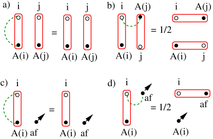
Figure 1: Action of singlet Projector (P, denoted by dashed line) in valence bond basis.

III Overlaps and operators

We now indicate the changes that arise in the formulae for the wavefunction overlaps between basis states, and for the action of exchange operators when working in the $S_{tot}=1/2$ sector. As is well-known, the wavefunction overlap between two bipartite VB basis states $|{\mathcal{P}}\rangle$ and $|{\mathcal{P}}^{\prime}\rangle$ of the singlet-sector basis are determined by the number of cycles needed to go from the permutation ${\mathcal{P}}$ to the permutation ${\mathcal{P}}^{\prime}$. More pictorially, one may consider the overlap diagram of the two valence-bond covers viewed as ‘complete dimer covers’ or ‘perfect’ matchings. This overlap diagram contains $N_{\mathrm{loop}}$ (closed) loops of various lengths $l_{\mu}$, such that each site is part of exactly one loop (see Fig 1). Knowing this overlap diagram, one may calculate the corresponding wavefunction overlap to be $\langle{\mathcal{P}}|{\mathcal{P}}^{\prime}\rangle=2^{N_{\mathrm{loop}}}/2^{N_{s}/2}$, where $N_{s}$, the total number of spins is assumed even.

Generalizing this to states in our basis for the $S_{tot}=1/2$ sector, we note that the corresponding picture is now terms of the overlap diagram of two partial valence bond covers $({\mathcal{A}},a_{f})$ and $({\mathcal{A}}^{\prime},a^{\prime}_{f})$, each of which leaves one site free (uncovered by a valence bond). Such an overlap diagram necessarily involves exactly one ‘open string’ of length $l_{f}$ connecting $a_{f}$ to $a^{\prime}_{f}$, in addition to $N_{\mathrm{loop}}$ (closed) loops of various lengths $l_{\alpha}$ (see Fig 1). An elementary calculation reveals that the wavefunction overlap in our $S_{tot}=1/2$ case is given as $\langle{\mathcal{A}}a_{f}\sigma|{\mathcal{A}}^{\prime}a^{\prime}_{f}\sigma^{\prime}\rangle=\delta_{\sigma\sigma^{\prime}}2^{N_{\mathrm{loop}}}/2^{(N_{s}-1)/2}$, with $N_{s}$, the number of sites, now taken to be odd.

The original singlet sector algorithm relies heavily Sandvik_prl05 ; Sandvik_Beach ; Sandvik_Evertz on a particularly simple action of operators $P_{ij}=\eta_{i}\eta_{j}{\mathbf{S}}_{i}\cdot{\mathbf{S}}_{j}+1/4$ on basis states $|{\mathcal{P}}\rangle$. Here $\eta_{i}=+1$ ($\eta_{i}=-1$) for $i$ belonging to the $A$-sublattice ($B$-sublattice), and thus, the operator $P_{a_{\alpha}b_{\beta}}$ that connects an $A$-sublattice site $a_{\alpha}$ to a $B$-sublattice site $b_{\beta}$ is precisely the projection operator that projects to the singlet state of the two spins ${\mathbf{S}}_{a_{\alpha}}$ and ${\mathbf{S}}_{b_{\beta}}$. Our key observation, which allows us to generalize this algorithm to the the $S_{tot}=1/2$ case, is that the action of $P_{ij}$ on states in our $S_{tot}=1/2$ basis remains simple. This is seen as follows: If neither $i$ nor $j$ correspond to the ‘free’ spin, $P_{ij}$ acts exactly as in the earlier singlet sector case (Fig 1(a,b)):

$${P_{{\mathcal{A}}(b_{\alpha})b_{\alpha}}}|...[{\mathcal{A}}(b_{\alpha})b_{\alpha}]...\;;a_{f}\uparrow\rangle = |...[{\mathcal{A}}(b_{\alpha}),b_{\alpha}]...\;;a_{f}\uparrow\rangle,$$

$${P_{{\mathcal{A}}(b_{\alpha})b_{\beta}}}|...[{\mathcal{A}}(b_{\alpha}),b_{\alpha}]...[{\mathcal{A}}(b_{\beta}),b_{\beta}]...\;;a_{f}\uparrow\rangle = \frac{1}{2}|...[{\mathcal{A}}(b_{\alpha}),b_{\beta}]...[{\mathcal{A}}(b_{\beta}),b_{\alpha}]...\;;a_{f}\uparrow\rangle,$$

$${P_{{\mathcal{A}}(b_{\alpha}){\mathcal{A}}(b_{\beta})}}|...[{\mathcal{A}}(b_{\alpha}),b_{\alpha}]...[{\mathcal{A}}(b_{\beta}),b_{\beta}]...\;;a_{f}\uparrow\rangle = \frac{1}{2}|...[{\mathcal{A}}(b_{\alpha}),b_{\beta}]...[{\mathcal{A}}(b_{\beta}),b_{\alpha}]...\;;a_{f}\uparrow\rangle,$$

$${P_{b_{\alpha}b_{\beta}}}|...[{\mathcal{A}}(b_{\alpha}),b_{\alpha}]...[{\mathcal{A}}(b_{\beta}),b_{\beta}]...\;;a_{f}\uparrow\rangle = \frac{1}{2}|...[{\mathcal{A}}(b_{\alpha}),b_{\beta}]...[{\mathcal{A}}(b_{\beta}),b_{\alpha}]...\;;a_{f}\uparrow\rangle.$$

On the other hand, if either $i$ or $j$ correspond to the free site $a_{f}$, one can easily check that the following holds (Fig 1(c,d)):

$${P_{a_{f}b_{\alpha}}}|...[{\mathcal{A}}(b_{\alpha})b_{\alpha}]...\;;a_{f}\uparrow\rangle = \frac{1}{2}|...[a_{f},b_{\alpha}]...\;;{\mathcal{A}}(b_{\alpha})\uparrow\rangle,$$

$${P_{a_{f}{\mathcal{A}}(b_{\alpha}})}|...[{\mathcal{A}}(b_{\alpha})b_{\alpha}]...\;;a_{f}\uparrow\rangle = \frac{1}{2}|...[a_{f},b_{\alpha}]...\;;{\mathcal{A}}(b_{\alpha})\uparrow\rangle.$$

Thus $P_{ij}$ either causes no change or rearranges exactly one pair of valence bonds to give a new basis state with amplitude $1/2$, or reconnects one valence bond to move the free spin to give a new basis state, again with amplitude $1/2$. The important thing to note is that these rules are in complete analogy to the original singlet sector case.

By analogy to the original singlet sector work Sandvik_prl05 ; Sandvik_Beach ; Sandvik_Evertz , this allows us to formulate a convenient prescription for the calculation of $\langle{\mathcal{A}}^{\prime}a^{\prime}_{f}\uparrow|P_{ij}|{\mathcal{A}}a_{f}\uparrow\rangle$ between two of our basis states by writing $\langle{\mathcal{A}}^{\prime}a^{\prime}_{f}\uparrow|P_{ij}|{\mathcal{A}}a_{f}\uparrow\rangle=W_{ij}\langle{\mathcal{A}}^{\prime}a^{\prime}_{f}\uparrow|{\mathcal{A}}a_{f}\uparrow\rangle$ and developing rules for the weight $W_{ij}$ by comparing the overlap diagram of $({\mathcal{A}}^{\prime}a^{\prime}_{f}\uparrow)$ and $(P_{ij}|{\mathcal{A}}a_{f}\uparrow)$ with the original overlap diagram of $({\mathcal{A}}^{\prime}a^{\prime}_{f}\uparrow)$ and $({\mathcal{A}}a_{f}\uparrow)$: If the action of $P_{ij}$ makes no changes in the original overlap diagram, $W_{ij}=1$. In addition, $W_{ij}=2\times 1/2=1$ if a loop is split into two loops or the open string is split into one loop and another open string; here, the factor of two comes from the fact that the number of loops in the overlap diagram increases by one, while the factor of half has its origins in the reconnection amplitude of one-half in Eqn LABEL:reconnectionamplitude. On the other hand, if two loops fuse into one, or if the open string fuses with a loop to give a larger open string, then $W_{ij}=(1/2)\times(1/2)$, where the first factor of half reflects the fact that the number of loops is reduced by one, while the second factor of one-half comes from the reconnection amplitude in Eqn LABEL:reconnectionamplitude. These rules are tabulated in Fig 2, and the important thing to note is that the open string can be treated on equal footing with (closed) loops in all cases, allowing one to generalize the singlet sector rules directly to the $S_{tot}=1/2$ sector case discussed here.

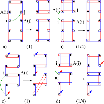
Figure 2: Action of a singlet projector on the overlap loops for closed loops (a, b) and open string (c,d). Corresponding weights are given below within parenthesis.

IV Generalization of the Sandvik-Evertz algorithm

With all of this in hand, it is now easy to see that the singlet sector algorithm of Sandvik and collaborators Sandvik_prl05 ; Sandvik_Beach ; Sandvik_Evertz generalizes straightforwardly to the $S_{tot}=1/2$ sector case for Hamiltonians of the form $H=-\sum_{b}H_{b}$, where each piece $-H_{b}$ of the Hamiltonian is a projector $P_{b_{1}b_{2}}$ acting on bond $b$ connecting spins $b_{1}$ and $b_{2}$. We start with an arbitrary $S_{tot}=1/2$ $S^{z}_{tot}=1/2$ state $|\psi_{1/2\uparrow}\rangle$, say $|\psi_{1/2\uparrow}\rangle=|{\mathcal{A}}a_{f}\uparrow\rangle$. As in the original singlet sector algorithm, we wish to stochastically sample $\langle\psi_{1/2\uparrow}|(-H)^{2m}|\psi_{1/2\uparrow}\rangle$ by sampling all possible operator strings $\prod_{\tau=1}^{2m}H_{b_{\tau}}$ in the decomposition of $(-H)^{2m}$ into a sum of products, with weight for each such string being proportional to $\langle\psi_{1/2\uparrow}|\prod_{\tau=1}^{2m}H_{b_{\tau}}|\psi_{1/2\uparrow}\rangle$. To do this, one splits each $H_{b}$ into a term $H_{b}^{\sigma=d}$ that is diagonal in the $\{S^{z}_{i}\}$ eigenbasis, and a term $H_{b}^{\sigma=o}$ that is offdiagonal. In addition, one writes $|\psi_{1/2\uparrow}\rangle$ in this basis as $|\psi_{1/2\uparrow}\rangle=\sum_{\{S^{z}_{i}\}}C_{\{S^{z}_{i}\}\uparrow}|\{S^{z}_{i}\}\rangle$. As in the original singlet sector case, each term $C_{\{{S^{z}_{i}}^{\prime}\}\uparrow}C_{\{S^{z}_{i}\}\uparrow}\langle\{{S^{z}_{i}}^{\prime}\}|\prod_{\tau=1}^{2m}H^{\sigma_{\tau}}_{b_{\tau}}|\{S^{z}_{i}\}\rangle$ is generated by working in a ‘spacetime’ loop representation and using a combination of ‘diagonal updates’ in which some $H^{\sigma_{\tau}=d}_{b_{\tau}}$ is moved to a different bond $b_{tau}^{\prime}$ and ‘loop updates’ whereby each space-time loop is flipped with probability half; this loop update allows one to switch between diagonal and off-diagonal pieces of a given set of bond operators, while simultaneously sampling all possible spin configurations $\left\{S^{z}_{i}\right\}$ in the state at $\tau=0$ and $\tau=2m$. The only difference with the original singlet sector case is that we now have precisely one open string in the space-time diagram, which connects the ‘free spin at $\tau=0$’, i.e the unpaired spin in $|\psi_{1/2}\uparrow\rangle$ to the ‘free spin at $\tau=2m$’, i.e the unpaired spin in $\langle\psi_{1/2}\uparrow|$, and which cannot be flipped, since the unpaired spins in all our $S_{tot}=1/2$, $S^{z}_{tot}=1/2$ basis states have fixed $z$ projection of $+1/2$. Finally, as in the singlet case, we can easily generalize this procedure to treat Hamiltonians that also contain products $-P_{b}P_{b^{\prime}}$ of projectors $P$ acting on distinct bonds $b$ and $b^{\prime}$ of the lattice.

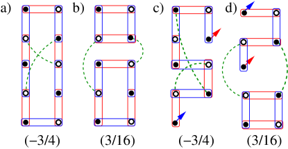
Figure 3: Overlap graphs contributing to the estimator of $\langle({\vec{m}^{2}})^{2}\rangle\equiv\sum_{ijkl}(P_{ij}-1/4)(P_{kl}-1/4)\rangle$ with corresponding values of $W_{ijkl}-W_{ij}W_{kl}$ (defined in text) given within parenthesis.

V Estimators

As in the singlet sector case Sandvik_prl05 ; Sandvik_Beach ; Sandvik_Evertz , physical properties can be calculated by taking each space-time loop diagram generated by the algorithm and ‘cutting it at $\tau=m$’ to obtain the overlap diagram that represents the overlap of $\prod_{\tau=1}^{m}H^{\sigma_{\tau}}_{b_{\tau}}|\psi_{1/2\uparrow}\rangle$ with $\langle\psi_{1/2\uparrow}\prod_{\tau=m+1}^{2m}H^{\sigma_{\tau}}_{b_{\tau}}$.

Consider for instance the Neel order parameter $\vec{m}=\sum_{i}\eta_{i}\vec{S}_{i}$. Clearly, $\langle m_{x}\rangle=\langle m_{y}\rangle=0$. However, $\langle m_{z}\rangle$ receives contributions from sites on the open string in the overlap diagram, since the open string, in contrast to (closed) loops, has only one orientation and therefore cannot be flipped. More formally, we may write $\langle{\mathcal{A}}^{\prime}a^{\prime}_{f}\uparrow|S^{z}_{i}|{\mathcal{A}}a_{f}\uparrow\rangle=W_{i}\langle{\mathcal{A}}^{\prime}a^{\prime}_{f}\uparrow|{\mathcal{A}}a_{f}\uparrow\rangle$ and note that $W_{i}=\eta_{i}/2$ if $i$ is part of the open string in the overlap diagram between $({\mathcal{A}}^{\prime}a^{\prime}_{f})$ and $({\mathcal{A}}a_{f})$ and $0$ otherwise. We thus find $\langle m_{z}\rangle=\langle l_{f}\rangle$, where the angular brackets on the right denote the ensemble average over the ensemble of overlap diagrams generated by the modified $S_{tot}=1/2S_{tot}^{z}=1/2$ sector algorithm outlined above.

We now turn to $\langle\vec{m}^{2}\rangle=\langle\sum_{ij}(P_{ij}-1/4)\rangle$. As noted earlier, whenever $i$ and $j$ are both in the open string or the same (closed) loop, the corresponding weight $W_{ij}=1$, while $W_{ij}=1/4$ when $i$ and $j$ do not both belong to the open string or the same (closed) loop. For an overlap diagram with closed loops of lengths $l_{\alpha}$ (with $\alpha=1,2\dots N_{l}-1$) and an open string of length $l_{N_{l}}\equiv l_{f}$, the latter can occur in $\sideset{}{{}^{\prime}}{\sum}_{\alpha,\beta=1}^{N_{l}}l_{\alpha}l_{\beta}$ ways where the prime on the sum indicates that $\alpha=\beta$ is disallowed, while the former can occur in $\sum_{\alpha=1}^{N_{l}}l_{\alpha}^{2}$ ways. As in the singlet sector case, we thus obtain $\langle\vec{m}^{2}\rangle=\langle\frac{1}{4}\sideset{}{{}^{\prime}}{\sum}_{\alpha,\beta=1}^{N_{l}}l_{\alpha}l_{\beta}+\sum_{\alpha=1}^{N_{l}}l_{\alpha}^{2}-\frac{1}{4}\sum_{\alpha,\beta=1}^{N_{l}}l_{\alpha}l_{\beta}$, where the angular brackets on the right indicate average over the ensemble of overlap diagrams generated by the algorithm. This reduces to

$$\langle m^{2}\rangle = \langle\frac{3}{4}\sum_{\alpha=1}^{N_{l}}l_{\alpha}^{2}\rangle$$ (8)

where the angular brackets on the right again denote averaging over the ensemble of overlap diagrams generated by the algorithm, and the important thing to note is that this estimator treats the open string ($\alpha=N_{l}$) on the same footing as the closed loops ($\alpha=1,2,\dots N_{l}-1$).

Finally, we consider the ground state expectation value of the fourth power of the Neel order parameter, i.e $\langle(\vec{m}^{2})^{2}\rangle$. To derive the estimator for this in the $S_{tot}=1/2$, $S^{z}_{tot}=1/2$, we follow Sandvik and Beach Sandvik_Beach , and write $\langle(\vec{m}^{2})^{2}\rangle=\langle\sum_{ij}\sum_{kl}(P_{ij}-1/4)(P_{kl}-1/4)\rangle$. As in Ref Sandvik_Beach, , we note that the estimator for this quantity differs from the square of the estimator for $\vec{m}^{2}$ only when the action of $P_{ij}$ ‘interferes’ with the action of $P_{kl}$, i.e when the actual weight $W_{ijkl}\equiv\langle{\mathcal{A}}^{\prime}a^{\prime}_{f}\uparrow|P_{ij}P_{kl}|{\mathcal{A}}a_{f}\uparrow\rangle/\langle{\mathcal{A}}^{\prime}a^{\prime}_{f}\uparrow|{\mathcal{A}}a_{f}\uparrow\rangle$ differs from the product $W_{ij}W_{kl}$ of the independent weights $W_{ij}\equiv\langle{\mathcal{A}}^{\prime}a^{\prime}_{f}\uparrow|P_{ij}|{\mathcal{A}}a_{f}\uparrow\rangle/\langle/{\mathcal{A}}^{\prime}a^{\prime}_{f}\uparrow|{\mathcal{A}}a_{f}\uparrow\rangle$ and $W_{kl}$ (defined analogously to $W_{ij}$). As in the singlet sector case, this happens only in the two cases shown in Fig 3, where the difference $W_{ijkl}-W_{ij}W_{kl}$ has been tabulated. Thus, the only new calculation needed is a count of the number of ways in which each of the cases Fig 3 (a), (b), (c), (d) arise, weighted by the corresponding values of $W_{ijkl}-W_{ij}W_{kl}$. It is at this step that the open string needs to be treated separately, since we find that this count for a open string in Fig 3 (c) differs from the analogous count for a closed loop in Fig 3 (a) by precisely one: Fig 3 (a) can arise in $\frac{1}{3}l_{\alpha}^{4}-\frac{4}{3}l_{\alpha}^{2}$ ways, while Fig 3 (c) can arise in $\frac{1}{3}l_{f}^{4}-\frac{4}{3}l_{f}^{2}+1$ ways. On the other hand, both Fig 3 (b) and (d) arise in precisely $2l_{\alpha}^{2}l_{\beta}^{2}$ ways (with $l_{\beta}\equiv l_{f}$) for Fig 3 (d).

With all this in hand, we obtain

$$\langle(\vec{m}^{2})^{2}\rangle = \left(\frac{3}{4}\sum_{\alpha=1}{N_{l}}l_{\alpha}^{2}\right)^{2}+$$ (9)

$$\frac{6}{16}\sideset{}{{}^{\prime}}{\sum}_{\alpha,\beta=1}^{N_{l}}l_{\alpha}^{2}l_{\beta}^{2}-\frac{1}{4}\sum_{\alpha=1}^{N_{l}}(l_{\alpha}^{4}-4l_{\alpha}^{2})-\frac{3}{4}\;,$$

which reduces to .

$$\langle(\vec{m}^{2})^{2}\rangle = \sum_{\alpha=1}^{N_{l}}{(-\frac{5}{8}l_{\alpha}^{4}+l_{\alpha}^{2})}+\frac{15}{16}(\sum_{\alpha=1}^{N_{l}}{l_{\alpha}^{2}})^{2}-\frac{3}{4}.$$

Again, the thing to note is that the presence of the open string only changes the estimator by an addition constant $-\frac{3}{4}$ when compared to the corresponding expression in the singlet sector case Sandvik_Beach .

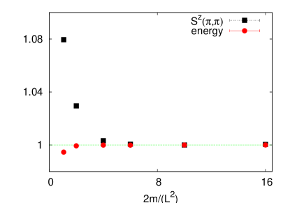
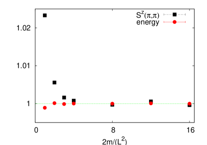
Figure 4: Variation of the ratio of Monte Carlo estimates of $S_{z}(\pi,\pi)$ and energy to exact values as a function of projection length: for a $3\times 5$ open system (top) and a $4\times 4$ periodic system (below).

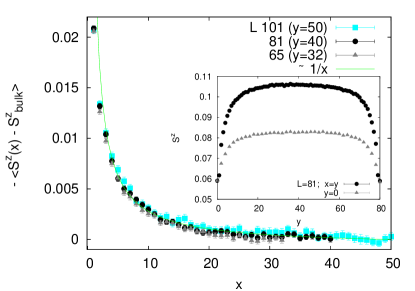
Figure 5: Boundary induced spin texture decays as $\sim 1/x$ to the bulk value along a direction perpendicular to the boundary: negative differences from bulk value shown along a cut perpendicular to the boundary for various systemsizes. Inset shows the $<S^{z}(x,y)>$ texture on the A-sublattice sites along a diagonal and an edge of a $81\times 81$ system.

VI Illustrative results and outlook

By way of illustration, we show results for a $L_{x}\times L_{y}$ square lattice Heisenberg antiferromagnet with $L_{x}$, $L_{y}$ odd and open boundary conditions, and for a $L\times L$ square lattice Heisenberg antiferromagnet with periodic boundary conditions and $L$ even, but with one site missing.

To benchmark the method, we first compare the results for $L_{x}=3$, $L_{y}=5$ open boundary condition system and a $L=4$ period boundary condition system having one site missing with the corresponding exact diagonalization results. In Fig 4, we show the dependence of the estimators for ground state energy, $S_{z}(\pi,\pi)$ and $\vec{m}_{s}^{2}$ as a function of the projection power $m$; this performance is comparable to the performance of the original algorithm in the singlet sector, and thus our modification provides a viable method to study antiferromagnets forced to have a $S_{tot}=1/2$ ground state due to the nature of the finite sample.

With this in hand, we move on to some illustrative physics results. For purposes of illustration, we consider a large open boundary condition system with an odd number of sites. In Fig 5 shows the magnetization at all sites of A sublattice for a open system with sizes $L=$. As noted by Metlitski and Sachdev Metlitski_Sachdev , the effect of the boundary is to decrease the sublattice magnetization near it which is then restored to its bulk value away from boundary in a power-law manner Hoglund_Sandvik ; Metlitski_Sachdev . As demonstrated by Ref Metlitski_Sachdev, , this suppression goes away as a power law $1/|\vec{r}|$ as a function of distance $|\vec{r}|$ from the edge. Using our method, we can directly calculate $\langle S(\vec{r})\rangle$ in an odd by odd square lattice. On general grounds, one expects that $(-1)^{\vec{r}}\langle S(\vec{r})\rangle$ will also obey this prediction of Metlitski and Sachdev, although this quantity is not directly related to the usual definition of the Neel order parameter. With this in mind, we compare our results with the predictions from Ref Metlitski_Sachdev, , and find extremely good agreement, pointing to the usefulness of our approach.

VII Acknowledgements

We acknowledge computations resources of TIFR, and funding from DST-SRC/S2/RJN-25/2006.

References

• (1) A.Β W.Β Sandvik, Phys. Rev. Lett. 95, 207203 (2005).
• (2) K.Β S.Β D.Β Beach and A.W. Sandvik, Nucl. Phys. B750, 142 (2006).
• (3) A.Β W.Β Sandvik and H.-G.Β Evertz, arXiv:0807.0682, unpublished.
• (4) A. W. Sandvik, Phys. Rev. B 59, R14157 (1999).
• (5) E. Manousakis, Rev. Mod. Phys. 63, 1 (1991).
• (6) N. V. Prokof’ev, B. V. Svistunov, and I. S. Tupitsyn, Pis’ma Zh. Eksp. Teor. Fiz. 64, 853 (1996)[Sov. Phys. JETP Lett. 64, 911 (1996)].
• (7) S.Β R.Β White,Phys. Rev. Lett. 69, 2863(1992).
• (8) G. Evenbly and G. Vidal, Phys. Rev. Lett. 102, 180406 (2009).
• (9) H. Alloul, J. Bobroff, M. Gabay, and P. Hirschfeld, Rev. Mod. Phys. 81, 45 (2009).
• (10) O. P. Vajk, P. K. Mang, M. Greven, P. M. Gehring, and J. W. Lynn, 2002, Science 295, 1691.
• (11) K. H. Huglund, and A W Sandvik, Phys. Rev. B 79, 020405 (2009).
• (12) M. A. Metlitski and S. Sachdev, Phys. Rev. B 77, 054411 (2008)