Onsager coefficients of a Brownian Carnot cycle

Abstract

We study a Brownian Carnot cycle introduced by T. Schmiedl and U. Seifert [Europhys. Lett. 81, 20003 (2008)] from a viewpoint of the linear irreversible thermodynamics. By considering the entropy production rate of this cycle, we can determine thermodynamic forces and fluxes of the cycle and calculate the Onsager coefficients for general protocols, that is, arbitrary schedules to change the potential confining the Brownian particle. We show that these Onsager coefficients contain the information of the protocol shape and they satisfy the tight-coupling condition irrespective of whatever protocol shape we choose. These properties may give an explanation why the Curzon-Ahlborn efficiency often appears in the finite-time heat engines.

I Introduction

Thermodynamics has been developed from the analysis of heat engines. Carnot invented an idealized mathematical model of heat engines, now called the Carnot cycle, and proved that there exists a fundamental upper bound of the efficiency of all heat engines, which is given by the Carnot efficiency $\eta_{\mathrm{C}}\equiv 1-T_{\mathrm{c}}/T_{\mathrm{h}}$, where $T_{\mathrm{h}}$ and $T_{\mathrm{c}}$ are the temperatures of the hotter and the colder heat reservoirs, respectively. But to attain the upper bound, we need to operate the heat engines infinitely slowly (quasistatic limit) not to cause irreversibility. In the quasistatic limit, the heat engine is of no practical use, because the power, defined as work output per unit time, becomes $0$.

Practically we need to operate the heat engines in a finite time to obtain a finite power. Curzon and Ahlborn CA considered a phenomenological model of a finite-time Carnot heat engine under the assumptions that heat flow obeys the linear Fourier law and that irreversibility occurs only due to the heat flow (endoreversible approximation) (see also C ; N ), and they derived that the efficiency at the maximal power $\eta_{\mathrm{max}}$ of that engine becomes

$$\eta_{\mathrm{max}}=1-\sqrt{\frac{T_{\mathrm{c}}}{T_{\mathrm{h}}}}\equiv\eta_{\mathrm{CA}}.$$ (1)

(Curzon-Ahlborn (CA) efficiency)

Although their derivation of $\eta_{\mathrm{CA}}$ may seem model-specific, they suggested that $\eta_{\mathrm{CA}}$ closely approximates $\eta_{\mathrm{max}}$ in a few examples of real heat engines CA and, above all, the simple form Eq. (1) of $\eta_{\mathrm{CA}}$ implied its universality. In fact, subsequent various theoretical studies indeed revealed some sort of universality of the CA efficiency R1 ; R2 ; LL ; G ; K ; B ; AB ; AB2 ; VB ; CH ; CH2 ; GS ; BK ; BB ; TYJ ; REC ; B2 ; IO ; IO2 ; IO3 ; SS ; TU ; ELB ; ELB2 ; BJM ; AJM ; J ; EKLB ; ZS .

Recently Van den Broeck addressed the generality of the CA efficiency from a viewpoint of the linear irreversible thermodynamics VB . He described heat engines by using the Onsager relations

$$J_{1}=L_{11}X_{1}+L_{12}X_{2},$$ (2)

$$J_{2}=L_{21}X_{1}+L_{22}X_{2},$$ (3)

and proved that $\eta_{\mathrm{CA}}$ is the upper bound of the efficiency at the maximal power $\eta_{\mathrm{max}}$ in the linear response regime $\Delta T\to 0$, where $\Delta T\equiv T_{\mathrm{h}}-T_{\mathrm{c}}$. This upper bound can be attained when the Onsager coefficients $L_{ij}$’s in Eqs. (2) and (3) satisfy the tight coupling condition $|q|=1$, where $q\equiv L_{12}/\sqrt{L_{11}L_{22}}$ is called the coupling strength parameter. Various theoretical models of the heat engines can be understood by using the Onsager relations, ranging from steady state Brownian motors GS ; BK ; B2 ; BB ; TYJ ; REC to a macroscopic finite-time Carnot cycle IO3 .

Recently Schmiedl and Seifert suggested an analytically tractable model of a Carnot heat engine from which useful work can be extracted through the motion of a Brownian particle by changing the potential confining the particle SS . In this paper, we call their model a Brownian Carnot cycle. By restricting the potential to the harmonic form, they analytically showed that the efficiency at the maximal power $\eta_{\mathrm{max}}$ agrees with $\eta_{\mathrm{CA}}$ in the limit of $\Delta T\to 0$. (See Sec. II for details.) The remarkable feature of their analysis is that they compared all protocols when maximizing the power, where we mean by protocol the schedule to change the potential.

Although they showed that their $\eta_{\mathrm{max}}$ attains $\eta_{\mathrm{CA}}$ in the linear response regime $\Delta T\to 0$, but the explicit Onsager relations Eqs. (2) and (3) have not been obtained yet, especially how the information of the protocol is reflected in the Onsager relations is unclear. In this paper, we calculate the Onsager coefficients $L_{ij}$’s of the Brownian Carnot cycle with the harmonic potential for general protocols, that is, arbitrary schedules to change the potential.

The organization of this paper is as follows. In Sec. II, we introduce the Brownian Carnot cycle and review its general properties according to SS . We demonstrate the calculations of its Onsager coefficients in Sec. III and discuss physical implications of them in Sec. IV. We summarize this study in Sec. V.

II Model

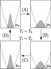
Figure 1: Schematic illustration of a Brownian Carnot cycle. A Brownian particle immersed in noisy thermal surroundings at temperature $T_{\mathrm{r}}$ is operated by changing the spring constant of the harmonic potential (dashed lines). The shadow regions represent the probability distribution $p(x,t)$. (A) and (C) are isothermal steps at $T_{\mathrm{r}}=T_{\mathrm{h}}$ and at $T_{\mathrm{r}}=T_{\mathrm{c}}$, respectively. (B) and (D) are instantaneous adiabatic steps which do not generate irreversibility. During the isothermal step (A) ((C)), $p(x,t)$ evolves according to the Fokker-Planck equation from $p_{a}$ ($p_{b}$) to $p_{b}$ ($p_{a}$).

Let us introduce the Brownian Carnot cycle SS . Imagine that a one-dimensional overdamped Brownian particle is immersed in thermal surroundings at a temperature $T_{\mathrm{r}}$ ($\mathrm{r}=\mathrm{h},\mathrm{c}$) and is trapped in a harmonic potential. The surroundings behave like noise on the particle and fluctuate its position. Therefore its motion becomes probabilistic rather than deterministic. In this situation, the time evolution of the probability distribution $p(x,t)$ of the position $x$ of the particle at time $t$ can be described by the Fokker-Planck equation

$$\frac{\partial p(x,t)}{\partial t}=-\mu\frac{\partial}{\partial x}\cdot\biggl{[}-\frac{\partial}{\partial x}V(x,t)-T_{\mathrm{r}}\frac{\partial}{\partial x}\biggr{]}p(x,t),$$ (4)

where $V(x,t)$ is the potential energy, which is given by $V(x,t)=\lambda(t)x^{2}/2$, using the time-dependent spring constant $\lambda(t)$. $\mu$ is the mobility of the particle and we set the Boltzmann constant $k_{\mathrm{B}}$ as unity. We can construct a Brownian Carnot cycle in a statistical sense by using Eq. (4) as follows (see Fig. 1): (A). Isothermal step at $T_{\mathrm{r}}=T_{\mathrm{h}}$ ($0<t<t_{A}$): by changing the spring constant, we change the distribution function from initial $p_{a}(x)$ to $p_{b}(x)$ for the duration of $t_{A}$. (B). Adiabatic step: at time $t=t_{A}$, we switch the reservoir at $T_{\mathrm{h}}$ to a colder one at $T_{\mathrm{c}}$ instantaneously. Because this instantaneous adiabatic step gives the probability distribution no time to relax, the probability distribution remains $p=p_{b}(x)$ during this step. (C). Isothermal step at $T_{\mathrm{r}}=T_{\mathrm{c}}$ ($t_{A}<t<t_{A}+t_{C}$): by changing the spring constant, we change the distribution function from $p_{b}(x)$ to $p_{a}(x)$ for the duration of $t_{C}$. (D). Adiabatic step: at time $t=t_{C}$, we switch the reservoir at $T_{\mathrm{c}}$ to the one at $T_{\mathrm{h}}$ instantaneously again. This adiabatic step also keeps the probability distribution as $p=p_{a}(x)$ and then the cycle closes. Since $\lambda(t)$ determines the schedule to change the potential, we consider $\lambda(t)$ as the protocol in this Brownian Carnot cycle. During the isothermal steps (A) and (C), the probability distribution evolves according to the Fokker-Planck equation Eq. (4) and we also assume that the initial probability $p_{a}(x)$ is Gaussian with the mean $0$ and the variance $w_{a}$ as $p_{a}(x)=\exp(-x^{2}/(2w_{a}))/\sqrt{2\pi w_{a}}$. Then it can be shown that the probability distribution always remains Gaussian with the mean $0$ in the case of the harmonic potential if we initially prepare it so.

Here we define the internal energy $E(t)$ and the entropy $S(t)$ of the particle at time $t$ as

$$E(t)\equiv\int_{-\infty}^{\infty}dx\ p(x,t)V(x,t),$$ (5)

$$S(t)\equiv-\int_{-\infty}^{\infty}dx\ p(x,t)\ln p(x,t),$$ (6)

respectively. The entropy $S$ of the particle does not change during the adiabatic steps (B) and (D) because the probability distribution remains unchanged. Thus the adiabatic steps are surely isentropic, which do not generate irreversibility during them at all.

To calculate the work output during the cycle, we consider the time evolution equation of the variance $w(t)\equiv\int_{-\infty}^{\infty}dx\ p(x,t)x^{2}$ during the isothermal steps (A) and (C) by using Eq. (4) as

$$\frac{dw^{(A)}}{dt}=-2\mu\lambda w^{(A)}+2\mu T_{\mathrm{h}}\ (0<t<t_{A}),$$ (7)

$$\frac{dw^{(C)}}{dt}=-2\mu\lambda w^{(C)}+2\mu T_{\mathrm{c}}\ (t_{A}<t<t_{A}+t_{C}),$$ (8)

where we have defined the variance during the isothermal steps (A) and (C) as $w^{(A)}$ and $w^{(C)}$, respectively. Then the work output in the isothermal step (A) ($0<t<t_{A}$) can be calculated by using Eq. (7) as

$$W^{(A)} =-\int_{0}^{t_{A}}dt\int_{-\infty}^{\infty}dx\ p(x,t)\frac{\partial V}{\partial t}$$ (9)

$$=-\int_{0}^{t_{A}}dt\ \frac{d\lambda}{dt}\frac{w^{(A)}}{2}$$

$$=-\frac{1}{4\mu}\int_{0}^{t_{A}}\frac{{(\frac{dw^{(A)}}{dt})}^{2}}{w^{(A)}}dt+\frac{1}{2}T_{\mathrm{h}}[\ln w^{(A)}]_{0}^{t_{A}}$$

$$-\frac{1}{2}[\lambda w^{(A)}]_{0}^{t_{A}}$$

$$\equiv-W_{\mathrm{irr}}^{(A)}+T_{\mathrm{h}}\Delta{S}^{(A)}-\Delta{E}^{(A)},$$

where $W_{\mathrm{irr}}^{(A)}\equiv\frac{1}{4\mu}\int_{0}^{t_{\mathrm{A}}}(\frac{dw^{(A)}}{dt})^{2}/w^{(A)}\ dt$ is the decrease of the work by irreversibility, which vanishes in the quasistatic limit $t_{A}\to\infty$. Assuming that the probability distribution $p$ is always Gaussian with the variance $w$, we have also defined the internal energy change and the entropy change during the isothermal step (A) as ${\Delta S}^{(A)}\equiv\frac{1}{2}[\ln w^{(A)}]_{0}^{t_{A}}$ and ${\Delta E}^{(A)}\equiv\frac{1}{2}[\lambda w^{(A)}]_{0}^{t_{A}}$, by using Eqs (5) and (6), respectively. The work output in the isothermal step (C) ($t_{A}<t<t_{A}+t_{C}$) can also be calculated likewise as

$$W^{(C)} =-\int_{t_{A}}^{t_{A}+t_{C}}dt\int_{-\infty}^{\infty}dx\ p(x,t)\frac{\partial V}{\partial t}$$ (10)

$$=-\int_{t_{A}}^{t_{A}+t_{C}}dt\ \frac{d\lambda}{dt}\frac{w^{(C)}}{2}$$

$$=-\frac{1}{4\mu}\int_{t_{A}}^{t_{A}+t_{C}}\frac{{(\frac{dw^{(C)}}{dt})}^{2}}{w^{(C)}}dt+\frac{1}{2}T_{\mathrm{c}}[\ln w]_{t_{A}}^{t_{A}+t_{C}}$$

$$-\frac{1}{2}[\lambda w^{(C)}]_{t_{A}}^{t_{A}+t_{C}}$$

$$\equiv-W_{\mathrm{irr}}^{(C)}+T_{\mathrm{c}}\Delta{S}^{(C)}-\Delta{E}^{(C)},$$

where $W_{\mathrm{irr}}^{(C)}$, ${\Delta S}^{(C)}$ and ${\Delta E}^{(C)}$ are defined in the same way as in the step (A). We need to determine the dynamics of $w^{(i)}(t)$ ($i=A,C$) to calculate $W_{\mathrm{irr}}^{(A)}$ and $W_{\mathrm{irr}}^{(C)}$ explicitly. Since the cyclic change of $\lambda(t)$ asymptotically leads to the Gaussian cyclic change of $p(x,t)$, $w^{(i)}(t)$ ($i=A,C$) is uniquely determined by $\lambda(t)$. Reversely, if we determine $w^{(i)}(t)$ ($i=A,C$), then the dynamics of $\lambda(t)$ is uniquely determined via Eqs. (7) and (8). Therefore we may regard $w^{(i)}(t)$ ($i=A,C$) as the protocol in this Brownian Carnot cycle instead of $\lambda(t)$.

The work outputs $W^{(B)}$ and $W^{(D)}$ in the adiabatic steps (B) ($t=t_{A}$) and (D) ($t=t_{A}+t_{C}$) simply become the change of the internal energy of the system as $W^{(B)}=-\Delta E^{(B)}$ and $W^{(D)}=-\Delta E^{(D)}$ because the instantaneous change of the spring constant during the adiabatic steps does not affect the probability distribution. Then the total work output $W\equiv\sum_{i=A}^{D}W^{(i)}$ during the entire cycle (A)-(D) is summed as

$$W=-W^{(A)}_{\mathrm{irr}}-W^{(C)}_{\mathrm{irr}}+(T_{\mathrm{h}}-T_{\mathrm{c}})\Delta S,$$ (11)

where we have used relations $\sum_{i=A}^{D}\Delta E^{(i)}=0$ and $\sum_{i=A}^{D}\Delta S^{(i)}=0$ due to the periodicity of the system and have defined $\Delta S$ as

$$\Delta S\equiv\Delta S^{(A)}=-\Delta S^{(C)}=\ln\sqrt{\frac{w_{b}}{w_{a}}}.$$ (12)

The heat $Q_{\mathrm{h}}$ absorbed into the system from the hotter reservoir during the step (A) becomes

$$Q_{\mathrm{h}}\equiv\Delta E^{(A)}+W^{(A)}=T_{\mathrm{h}}\Delta S-W^{(A)}_{\mathrm{irr}}.$$ (13)

Here we define the power and the efficiency as

$$P\equiv\dot{W}\equiv\frac{W}{t_{A}+t_{C}},$$ (14)

$$\eta\equiv\frac{\dot{W}}{\dot{Q}_{\mathrm{h}}},$$ (15)

where the dot denotes a quantity divided by the one-cycle period or a quantity per unit time throughout the paper. In the Brownian Carnot cycle, the one-cycle period is $t_{A}+t_{C}$.

After the above setup for the Brownian Carnot cycle, Schmiedl and Seifert considered the maximization of the power as follows. Firstly they calculated the optimal protocol which maximizes the power Eq. (14) under the condition that the durations $t_{A}$ and $t_{C}$ and the boundary values $w_{a}$ and $w_{b}$ are fixed. This optimization can be realized by minimizing the functionals in $W^{(A)}_{\mathrm{irr}}$ and $W^{(C)}_{\mathrm{irr}}$ since $\Delta S$ in Eq. (11) is constant. By solving Euler-Lagrange equations for these functionals with given boundary values $w_{a}$ and $w_{b}$, they obtained the optimal protocol as

$$w^{(A)}(t) =w_{a}(1+(\sqrt{w_{b}/w_{a}}-1)t/t_{A})^{2},$$ (16)

$$w^{(C)}(t) =w_{b}(1+(\sqrt{w_{a}/w_{b}}-1)(t-t_{A})/t_{C})^{2}.$$ (17)

Then, $W^{(A)}_{\mathrm{irr}}$ and $W^{(C)}_{\mathrm{irr}}$ under this protocol are expressed as

$$W^{(A)}_{\mathrm{irr}}=\frac{(\sqrt{w_{b}}-\sqrt{w_{a}})^{2}}{\mu}\cdot\frac{1}{t_{A}},$$ (18)

$$W^{(C)}_{\mathrm{irr}}=\frac{(\sqrt{w_{b}}-\sqrt{w_{a}})^{2}}{\mu}\cdot\frac{1}{t_{C}}.$$ (19)

Secondly they considered the further maximization of the power of the optimal protocol by changing the durations $t_{A}$ and $t_{C}$. From $\partial P/\partial t_{A}=\partial P/\partial t_{C}=0$, $t_{A}$ and $t_{C}$ can be determined as

$$t_{A}=t_{C}=\frac{4(\sqrt{w_{b}}-\sqrt{w_{a}})^{2}}{\mu(T_{\mathrm{h}}-T_{\mathrm{c}})\Delta S}.$$ (20)

Finally, they obtained the maximal power $P_{\mathrm{max}}$ and the efficiency at the maximal power $\eta_{\mathrm{max}}$ as

$$P_{\mathrm{max}}=\frac{\mu\left(\ln\sqrt{{w_{b}}/{w_{a}}}\right)^{2}{\Delta T}^{2}}{16(\sqrt{w_{b}}-\sqrt{w_{a}})^{2}},$$ (21)

$$\eta_{\mathrm{max}}=\frac{\eta_{\mathrm{C}}}{2-\eta_{\mathrm{C}}/2},$$ (22)

where $\eta_{\mathrm{C}}=1-T_{\mathrm{c}}/T_{\mathrm{h}}$ is the Carnot efficiency. This result is remarkable because $\eta_{\mathrm{max}}$ is independent of the boundary values $w_{a}$ and $w_{b}$, although $P_{\mathrm{max}}$ depends on them. Thus, this implies that $\eta_{\mathrm{max}}$ in Eq. (22) remains unchanged even when the further maximization of the power is performed by changing $w_{a}$ and $w_{b}$ in Eq. (21). Therefore, $\eta_{\mathrm{max}}$ in Eq. (22) gives the efficiency at the maximal power under arbitrary protocols of $w(t)$.

Moreover, by expanding $\Delta T$, they obtained $\eta_{\mathrm{max}}=\Delta T/(2T)+O({\Delta T}^{2})$ which is equal to $\eta_{\mathrm{CA}}$ in the linear order of $\Delta T$. A remark should be added here. The essential point of their derivation is to consider the two-step maximization of the power: first by the optimal protocol for the fixed durations and second by those durations. This strategy to find the maximal power is indeed effective for the non-linear response regime of the cycle where we have no general theory to describe that regime at present. But we can use the linear irreversible thermodynamics in the linear order in $\Delta T$. As we will show in Sec. III, we indeed apply the framework of the linear irreversible thermodynamics to this Brownian Carnot cycle and can extract more detailed information on the maximization of the power in the linear response regime.

III Calculations of the Onsager coefficients

In this Section, we will calculate the Onsager coefficients of the Brownian Carnot cycle. Firstly we introduce the Onsager relations of a general linear irreversible heat engine VB . Let us consider that the heat engine is working under an external force $F$ and a small temperature difference $\Delta T$. The work performed against the external force $F$ is defined as $W=-Fx$, where $x$ is the thermodynamically conjugate variable of $F$. In the limit of the small temperature difference $\Delta T\to 0$, we can define a thermodynamic force $X_{1}=F/T_{\mathrm{c}}\simeq F/T$ where $T\equiv(T_{\mathrm{h}}+T_{\mathrm{c}})/2$ and its conjugate flux as $J_{1}=\dot{x}$. We also define the inverse temperature difference $1/T_{\mathrm{c}}-1/T_{\mathrm{h}}\simeq\Delta T/T^{2}$ as another thermodynamic force $X_{2}$ and the heat flux from the hotter heat reservoir $\dot{Q}_{\mathrm{h}}$ as its conjugate flux $J_{2}$. Moreover, we assume that the Onsager relations hold for these fluxes and forces as O ; GM

$$J_{1}=L_{11}X_{1}+L_{12}X_{2},$$ (23)

$$J_{2}=L_{21}X_{1}+L_{22}X_{2},$$ (24)

where $L_{ij}$’s are the Onsager coefficients with the symmetry relation $L_{12}=L_{21}$.

To write down the Onsager relations for the Brownian Carnot cycle, we need to choose the thermodynamic fluxes and forces for it. A typical way for choosing them is to consider the total entropy production rate $\dot{\sigma}$ during one cycle. Because the system entropy $S$ does not change after one cycle as $\sum_{i=A}^{D}\Delta S^{(i)}=0$, only the entropy increase in the reservoirs contributes to $\dot{\sigma}$ as

$$\dot{\sigma}\equiv-\frac{\dot{Q}_{\mathrm{h}}}{T_{\mathrm{h}}}-\frac{\dot{Q}_{\mathrm{c}}}{T_{\mathrm{c}}}=-\frac{\dot{Q}_{\mathrm{h}}}{T_{\mathrm{h}}}-\frac{\dot{W}-\dot{Q}_{\mathrm{h}}}{T_{\mathrm{c}}}.$$ (25)

In the linear response regime $\Delta T\to 0$, $\dot{\sigma}$ can be approximated as

$$\dot{\sigma}\simeq\frac{-W}{T}\cdot\frac{1}{(\alpha+1)t_{A}}+\frac{\Delta T}{T^{2}}\cdot\dot{Q}_{\mathrm{h}},$$ (26)

where we define $\alpha\equiv t_{C}/t_{A}$ as the ratio of $t_{C}$ to $t_{A}$ and we have neglected the higher terms like $O(\Delta T\dot{W})$ and $O(\Delta T^{3}\dot{Q}_{\mathrm{h}})$, whose reason will be clarified later. The expression $\dot{\sigma}=J_{1}X_{1}+J_{2}X_{2}$ by the linear irreversible thermodynamics leads to the decomposition of the thermodynamic forces as

$$X_{1}\equiv\frac{-W}{T},\ X_{2}\equiv\frac{\Delta T}{T^{2}}$$ (27)

and their conjugate fluxes as

$$J_{1}\equiv\frac{1}{(\alpha+1)t_{A}},\ J_{2}\equiv\dot{Q}_{\mathrm{h}}.$$ (28)

As is clear from these definitions for the thermodynamic fluxes and forces, we understand that the higher terms like $O(\Delta T\dot{W})$ and $O(\Delta T^{3}\dot{Q}_{\mathrm{h}})$ do not contribute to the entropy production rate $\dot{\sigma}$ in the linear response regime $\Delta T\to 0$. That’s why we neglected them in Eq. (26). By using these definitions for the thermodynamic fluxes and forces, we can write down the Onsager relations of the Brownian Carnot cycle as

$$\frac{1}{(\alpha+1)t_{A}} =L_{11}\frac{-W}{T}+L_{12}\frac{\Delta T}{T^{2}},$$ (29)

$$\dot{Q}_{\mathrm{h}} =L_{21}\frac{-W}{T}+L_{22}\frac{\Delta T}{T^{2}}.$$ (30)

Now we calculate the Onsager coefficients $L_{ij}$’s. First we calculate $L_{11}$ and $L_{21}$ as follows. By using a scaled variable $s\equiv t/t_{A}$ $(0<s<1)$ instead of $t$ ($0<t<t_{A}$) during the isothermal step (A), $W_{\mathrm{irr}}^{(A)}$ in Eq. (11) becomes

$$W_{\mathrm{irr}}^{(A)}=\frac{1}{t_{A}}\frac{1}{4\mu}\int_{0}^{1}\frac{(\frac{d\tilde{w}^{(A)}}{ds})^{2}}{\tilde{w}^{(A)}}ds\equiv\frac{A_{\mathrm{irr}}}{t_{A}},$$ (31)

where we call $\tilde{w}^{(A)}(s)\equiv w^{(A)}(t)$ the protocol shape. In Eq. (31), we have divided $W_{\mathrm{irr}}^{(A)}$ into the part proportional to the functional of the protocol shape $A_{\mathrm{irr}}$ and the duration $t_{A}$. $W_{\mathrm{irr}}^{(C)}$ during the isothermal step (C) in Eq. (11) can also be divided as

$$W_{\mathrm{irr}}^{(C)}=\frac{1}{t_{C}}\frac{1}{4\mu}\int_{0}^{1}\frac{(\frac{d\tilde{w}^{(C)}}{ds})^{2}}{\tilde{w}^{(C)}}ds\equiv\frac{C_{\mathrm{irr}}}{t_{C}}$$ (32)

by using a scaled variable $s\equiv(t-t_{A})/t_{C}$ ($0<s<1$) instead of $t$ ($t_{A}<t<t_{A}+t_{C}$) and $\tilde{w}^{(C)}(s)\equiv w^{(C)}(t)$. Then Eq. (11) can be expressed by using Eqs. (31) and (32) as

$$W=-\frac{1}{t_{A}}\Bigl{(}A_{\mathrm{irr}}+\frac{C_{\mathrm{irr}}}{\alpha}\Bigr{)}+\Delta T\Delta S.$$ (33)

By putting $\Delta T=0$ in Eq. (33), we can obtain the relation

$$\frac{1}{(\alpha+1)t_{A}}=\frac{T}{\left(A_{\mathrm{irr}}+C_{\mathrm{irr}}/{\alpha}\right)(\alpha+1)}\cdot\frac{-W}{T},$$ (34)

which determines the coefficient $L_{11}$ as

$$L_{11}=\frac{T}{\left(A_{\mathrm{irr}}+C_{\mathrm{irr}}/{\alpha}\right)(\alpha+1)}.$$ (35)

$\dot{Q}_{\mathrm{h}}$ at $\Delta T=0$ can also be calculated by using Eqs. (13) and (34) as

$$\dot{Q}_{\mathrm{h}}=\frac{T^{2}\Delta S}{\left(A_{\mathrm{irr}}+C_{\mathrm{irr}}/{\alpha}\right)(\alpha+1)}\cdot\frac{-W}{T}-\frac{A_{\mathrm{irr}}}{(\alpha+1){t_{A}}^{2}},$$ (36)

where the second term can be neglected because it is $O(W^{2})$ quantity from Eq. (34). Then the coefficient $L_{21}$ can be determined as

$$L_{21}=\frac{T^{2}\Delta S}{\left(A_{\mathrm{irr}}+C_{\mathrm{irr}}/{\alpha}\right)(\alpha+1)}.$$ (37)

Next we calculate $L_{12}$ and $L_{22}$ likewise. Putting $W=0$ in Eq. (33), we obtain the relation

$$\frac{1}{(\alpha+1)t_{A}}=\frac{T^{2}\Delta S}{\left(A_{\mathrm{irr}}+C_{\mathrm{irr}}/{\alpha}\right)(\alpha+1)}\cdot\frac{\Delta T}{T^{2}},$$ (38)

which determines the coefficient $L_{12}$ as

$$L_{12}=\frac{T^{2}\Delta S}{\left(A_{\mathrm{irr}}+C_{\mathrm{irr}}/{\alpha}\right)(\alpha+1)}.$$ (39)

From Eqs. (37) and (39), we find that the Onsager symmetry relation $L_{21}=L_{12}$ surely holds as expected. $\dot{Q}_{\mathrm{h}}$ at $W=0$ thus becomes

$$\dot{Q}_{\mathrm{h}}=\frac{T^{3}{\Delta S}^{2}}{\left(A_{\mathrm{irr}}+C_{\mathrm{irr}}/{\alpha}\right)(\alpha+1)}\cdot\frac{\Delta T}{T^{2}}-\frac{A_{\mathrm{irr}}}{(\alpha+1){t_{A}}^{2}}$$ (40)

from Eqs. (13) and (38), where the second term can be neglected because it is $O(\Delta T^{2})$ quantity from Eq. (38). Then the last coefficient $L_{22}$ turns out to be

$$L_{22}=\frac{T^{3}{\Delta S}^{2}}{\left(A_{\mathrm{irr}}+C_{\mathrm{irr}}/{\alpha}\right)(\alpha+1)}.$$ (41)

Note that these Onsager coefficients satisfy the constraints $L_{11}\geq 0$, $L_{22}\geq 0$ and $L_{11}L_{22}-L_{12}L_{21}\geq 0$ which come from the positivity of the entropy production rate $\dot{\sigma}$. We also note that although they are expressed in terms of $\tilde{w}$’s through $A_{\mathrm{irr}}$ and $C_{\mathrm{irr}}$, we could easily switch to the $\lambda$ representation by solving the differential equation Eqs. (7) and (8) explicitly and substituting the solutions $\tilde{w}$’s into $A_{\mathrm{irr}}$ and $C_{\mathrm{irr}}$.

IV Discussion

Now that we have calculated the Onsager coefficients of the Brownian Carnot cycle in Sec. III, we will discuss physical implications of them in this Section. To see how the Onsager relations are used to describe the efficiency and the power of the Brownian Carnot cycle, we introduce the general theory to describe the heat engines governed by the Onsager relations developed in VB as follows. Generally the power $P$ and the efficiency $\eta$ of the linear irreversible heat engine are expressed as

$$P =\dot{W}=-F\dot{x}=-J_{1}X_{1}T,$$ (42)

$$\eta =\frac{\dot{W}}{\dot{Q}_{\mathrm{h}}}=-\frac{J_{1}X_{1}T}{J_{2}},$$ (43)

respectively. When $X_{2}$ determined by the reservoir’s temperatures and the Onsager coefficients $L_{ij}$’s are given, we can see that only $X_{1}$ determines the power $P$ and the efficiency $\eta$. Since $X_{1}$ at the maximal power is given by $\partial P/\partial X_{1}=0$, we obtain $\eta_{\mathrm{max}}$ as

$$\eta_{\mathrm{max}}=\frac{\Delta T}{2T}\frac{q^{2}}{2-q^{2}},$$ (44)

where $q$ is defined as

$$q\equiv\frac{L_{12}}{\sqrt{L_{11}L_{22}}},$$ (45)

which is called the coupling strength parameter. Taking into account the restriction $-1\leq q\leq 1$ due to $L_{11}L_{22}-L_{12}L_{21}\geq 0$ which comes from the positivity of the entropy production rate $\dot{\sigma}$, $\eta_{\mathrm{max}}$ becomes the upper bound

$$\eta_{\mathrm{max}}=\frac{\Delta T}{2T}=\eta_{\mathrm{CA}}+O(\Delta T^{2})$$ (46)

when the tight coupling condition $|q|=1$ is satisfied.

As seen from Eqs. (31) and (32), we have shown that when we consider a protocol $w^{(i)}(t)$ by separating it into its shape $\tilde{w}^{(i)}(s)$ and its duration $t_{i}$, the Onsager coefficients Eqs. (35), (37), (39) and (41) of the Brownian Carnot cycle contain the information of the protocol shape through $A_{\mathrm{irr}}$ and $C_{\mathrm{irr}}$ and the thermodynamic flux $J_{1}$ is the inverse of the one-cycle period $(\alpha+1)t_{A}=t_{A}+t_{C}$. The remarkable feature is that as easily confirmed, they satisfy the tight coupling condition $|q|=1$, independently of the protocol shape, which means that the efficiency at the maximal power is always the CA efficiency. As we have shown above, this result is derived when the power is maximized by changing the thermodynamic force $X_{1}$. However, $X_{1}$ corresponds to $J_{1}$ via Eq. (29) at the fixed temperatures and protocol shape. Therefore, we can consider that changing $X_{1}$ is equivalent to changing $J_{1}$ or the one-cycle period. This leads to the result that in the present model of the Brownian Carnot cycle, the efficiency at the maximal power is always the CA efficiency when the power is maximized by changing only the one-cycle period with the protocol shape fixed. If the above feature of the Onsager coefficients is common to various heat engines, our result may explain the appearance of the CA efficiency found in  CA ; IO ; IO2 ; IO3 , where the power is maximized by changing only the one-cycle period without choosing the optimal protocol shape realizing the true maximal power.

The relation to the study by Schmiedl and Seifert SS reviewed in Sec. II can be understood as follows. Though in Eq. (46), we have seen that the efficiency at the maximal power $\eta_{\mathrm{max}}$ under an arbitrary protocol shape is $\eta_{\mathrm{CA}}$, the maximal power $P_{\mathrm{max}}$ should be lower than the true maximal power on the space of all protocol shapes. Here let us consider the further maximization of $P_{\mathrm{max}}$ obtained from the Onsager relations. Maximizing the power Eq. (42) by changing $X_{1}$, the maximal power $P_{\mathrm{max}}$ is given by

$$P_{\mathrm{max}}=\frac{L_{22}{\Delta T}^{2}}{4T^{3}}.$$ (47)

We notice that $L_{22}$ still depends on $\alpha$, $A_{\mathrm{irr}}$ and $C_{\mathrm{irr}}$. Then we can further maximize this $P_{\mathrm{max}}$ by minimizing the functionals in $A_{\mathrm{irr}}$ and $C_{\mathrm{irr}}$ with the boundary values $w_{a}$ and $w_{b}$, and also by changing $\alpha$, which reduces to an inequality

$$P_{\mathrm{max}}\leq\frac{\mu\left(\ln\sqrt{{w_{b}}/{w_{a}}}\right)^{2}{\Delta T}^{2}}{16(\sqrt{w_{b}}-\sqrt{w_{a}})^{2}}.$$ (48)

The equality is realized when $\alpha=1$ and $A_{\mathrm{irr}}=C_{\mathrm{irr}}=(\sqrt{w_{b}}-\sqrt{w_{a}})^{2}/\mu$, which corresponds to the case of the optimal protocol in Eqs. (16) and (17). The right-hand side of Eq. (48) is the maximal power that the cycle can output in the linear response regime at given boundary values $w_{a}$ and $w_{b}$ and is equal to Eq. (21). Thus the result in SS can be reproduced from the Onsager relations.

V summary

In summary, we derived the Onsager relations for a Brownian Carnot cycle working in the linear-response regime. We considered a protocol by separating it into its shape and its duration, where we mean by protocol the schedule to change the potential confining the Brownian particle. Then, we found that the Onsager coefficients contain the functionals of the protocol shape to change the potential and they satisfy the tight coupling condition, irrespective of whatever protocol shape we choose. This result implies that we can attain the Curzon-Ahlborn efficiency when maximizing the power by changing only the one-cycle period under an arbitrary protocol shape. In this sense, the Curzon-Ahlborn efficiency looks like the Carnot efficiency because the latter can also be attained irrespective of whatever protocol shape we choose in the quasistatic limit. Although we used the harmonic potential to construct the Brownian Carnot cycle, we believe that our results could also be applied to the models with general potentials and arbitrary dimensions discussed in SS , where the efficiency at the true maximal power agrees with the Curzon-Ahlborn efficiency. We expect that our study will stimulate the further discussion on the physics of the finite-time heat engines.

- (1) F. Curzon and B. Ahlborn, Am. J. Phys. 43, 22 (1975).
- (2) H. Callen, Thermodynamics and an Introduction to Thermostatistics (Wiley, New York, 1985), 2nd ed, Chap. 4.
- (3) I. I. Novikov, J. Nuclear Energy II 7, 125 (1958).
- (4) M. H. Rubin, Phys. Rev. A 19, 1272 (1979).
- (5) M. H. Rubin, Phys. Rev. A 19, 1277 (1979).
- (6) P. T. Landsberg and H. Leff, J. Phys. A 22, 4019 (1989).
- (7) J. M. Gordon, Am. J. Phys. 57, 1136 (1989).
- (8) R. Kosloff, J. Chem. Phys. 80, 1625 (1984).
- (9) A. Benjamin, J. Appl. Phys. 79, 1191 (1996).
- (10) M. Asfaw and M. Bekele, Eur. Phys. J. B 38, 457 (2004).
- (11) M. Asfaw and M. Bekele, Phys. Rev. E 72, 056109 (2005).
- (12) C. Van den Broeck, Phys. Rev. Lett. 95, 190602 (2005).
- (13) B. Jiménez de Cisneros and A. Calvo Hernández, Phys. Rev. Lett. 98, 130602 (2007).
- (14) B. Jiménez de Cisneros and A. Calvo Hernández, Phys. Rev. E 77, 041127 (2008).
- (15) A. Gomez-Marin and J. M. Sancho, Phys. Rev. E 74, (062102) (2006).
- (16) R. Benjamin and R. Kawai, Phys. Rev. E 77, 051132 (2008).
- (17) M. Van den Broeck and C. Van den Broeck, Phys. Rev. Lett. 100, 130601 (2008).
- (18) Gao Tian-Fu, Zhang Yue, and Chen Jin-Can, Chinese Phys. B. 18 3279 (2009).
- (19) R. Rutten, M. Esposito, and B. Cleuren, Phys. Rev. B 80, 235112 (2009).
- (20) R. Benjamin, arXiv: 0907.0829v1.
- (21) Y. Izumida and K. Okuda, Europhys. Lett. 83, 60003 (2008).
- (22) Y. Izumida and K. Okuda, Prog. Theor. Phys. Suppl. 178, 163-168 (2009).
- (23) Y. Izumida and K. Okuda, Phys. Rev. E 80, 021121 (2009).
- (24) T. Schmiedl and U. Seifert, Europhys. Lett. 81, 20003 (2008).
- (25) Z. C. Tu, J. Phys. A. 41, 312003 (2008).
- (26) M. Esposito, K. Lindenberg, and C. Van den Broeck, Europhys. Lett. 85, 60010 (2009).
- (27) M. Esposito, K. Lindenberg, and C. Van den Broeck, Phys. Rev. Lett. 102, 130602 (2009).
- (28) J. Birjukov, T. Jahnke and G. Mahler, Euro. Phys. J. B, 64, 105 (2008).
- (29) A. E. Allahverdyan, R. S. Johal, and G. Mahler, Phys. Rev. E 77, 041118 (2008).
- (30) R. S. Johal, Phys. Rev. E 80, 041119 (2009).
- (31) M. Esposito, R. Kawai, K. Lindenberg and C. Van den Broeck, Phys. Rev. E 81, 041106 (2010).
- (32) Y. Zhou and D. Segal, arXiv: 1002.2170v1.
- (33) L. Onsager, Phys. Rev. 37, 405 (1931).
- (34) S. R. de Groot and P. Mazur, Non-Equilibrium Thermodynamics (Dover, New York, 1984).