On population resilience to external perturbations

Abstract.

We study a spatially explicit harvesting model in periodic or bounded environments. The model is governed by a parabolic equation with a spatially dependent nonlinearity of Kolmogorov–Petrovsky–Piskunov type, and a negative external forcing term $-\delta$. Using sub- and supersolution methods and the characterization of the first eigenvalue of some linear elliptic operators, we obtain existence and nonexistence results as well as results on the number of stationary solutions. We also characterize the asymptotic behavior of the evolution equation as a function of the forcing term amplitude.

In particular, we define two critical values $\delta^{*}$ and $\delta_{2}$ such that, if $\delta$ is smaller than $\delta^{*}$, the population density converges to a “significant” state, which is everywhere above a certain small threshold, whereas if $\delta$ is larger than $\delta_{2}$, the population density converges to a “remnant” state, everywhere below this small threshold. Our results are shown to be useful for studying the relationships between environmental fragmentation and maximum sustainable yield from populations. We present numerical results in the case of stochastic environments.

1. Introduction

Overexploitation has led to the extinction of many species [5]. Traditionally, models of ordinary differential equations (ODEs) or difference equations have been used to estimate the maximum sustainable yields from populations and to perform quantitative analysis of harvesting policies and management strategies [18]. Ignoring age or stage structures as well as delay mechanisms, which will not be treated by the present paper, the ODEs models are generally of the type

(1.1) $$\frac{dU}{dt}=F(U)-Y(U),$$

where $U$ is the population biomass at time $t$, $F(U)$ is the growth function, and $Y(U)$ corresponds to the harvest function. In these models, the most commonly used growth function is logistic, with $F(U)=U(\mu-\nu U)$ (see [6], [26], [36]), where $\mu>0$ is the intrinsic growth rate of the population and $\nu>0$ models its susceptibility to crowding effects.

Different harvesting strategies $Y(U)$ have been considered in the literature and are used in practical resource management. A very common one is the constant-yield harvesting strategy, where a constant number of individuals are removed per unit of time: $Y(U)=\delta$, with $\delta$ a positive constant. This harvesting function naturally appears when a quota is set on the harvesters [32], [33], [39]. Another frequently used harvesting strategy is the proportional harvesting strategy (also called constant-effort harvesting), where a constant proportion of the population is removed. It leads to a harvesting function of the type $Y(U)=\delta U$.

Much less has been done in this field using reaction-diffusion models (but see [24], [27], [30]). The aim of this paper is to perform an analysis of some harvesting models, within the framework of reaction-diffusion equations.

One of the most celebrated reaction-diffusion models was introduced by Fisher [16] and Kolmogorov, Petrovsky, and Piskunov [23] in 1937 (we call it the Fisher-KPP model). Since then, it has been widely used to model spatial propagation or spreading of biological species into homogeneous environments (see books [26], [29], and [41] for a review). The corresponding equation is

(1.2) $$u_{t}=D\nabla^{2}u+u(\mu-\nu u),$$

where $u=u(t,x)$ is the population density at time $t$ and space position $x$, $D$ is the diffusion coefficient, and $\mu$ and $\nu$ still correspond to the constant intrinsic growth rate and susceptibility to crowding effects. In the 1980s, this model was extended to heterogeneous environments by Shigesada, Kawasaki, and Teramoto [38]. The corresponding model (which we call the SKT model in this paper) is of the type

(1.3) $$u_{t}=D\nabla^{2}u+u(\mu(x)-\nu(x)u).$$

The coefficients $\mu(x)$ and $\nu(x)$ now depend on the space variable $x$ and can therefore include some effects of environmental heterogeneity. More recently, this model revealed that the heterogeneous character of the environment plays an essential role in species persistence, in the sense that for different spatial configurations of the environment a population can survive or become extinct, depending on the habitat spatial structure [9], [13], [35], [37].

As mentioned above, the combination of a harvesting model with a Fisher-KPP population dynamics model, leading to an equation of the form $u_{t}=D\nabla^{2}u+u(\mu-\nu u)-Y(x,u)$, has been considered in recent papers, either using a spatially dependent proportional harvesting term $Y(x,u)=q(x)u$ in [27], [30], or a spatially dependent and time-constant harvesting term $Y(x)=h(x)$ in [24]. In these papers, the models were considered in bounded domains with Dirichlet (lethal) boundary conditions.

Here we study a population dynamics model of the SKT type, with a spatially dependent harvesting term $Y(x,u)$:

(1.4) $$u_{t}=D\nabla^{2}u+u(\mu(x)-\nu(x)u)-Y(x,u).$$

We mainly focus on a “quasi-constant-yield” case, where the harvesting term depends on $u$ only for very low population densities (ensuring the nonnegativity of $u$). We consider two types of domains and boundary conditions. In the first case, the domain is bounded with Neumann (reflective) boundary conditions; this framework is often more realistic for modeling species that cannot cross the domain boundary. In the second case, we consider the model (1.4) in the whole space $\mathbb{R}^{N}$ with periodic coefficients. This last situation, though technically more complex, is useful, for instance, for studying spreading phenomena [8], [10], and for studying the effects of environmental fragmentation, independently of the boundary effects. Lastly, note that the effects of variability in time of the harvesting function will be investigated in a forthcoming publication [14].

In section 2, we define a quasi-constant-yield harvesting reaction-diffusion model. We prove, on a firm mathematical basis, existence and nonexistence results for the equilibrium equations, as well as results on the number of possible stationary states. We also characterize the asymptotic behavior of the solutions of (1.4). In section 3, we illustrate the practical usefulness of the results of section 2, by studying the effects of the amplitude of the harvesting term on the population density in terms of environmental fragmentation. Lastly, in section 4, we give new results for the proportional harvesting case $Y(x,u)=q(x)u$.

2. Mathematical analysis of a quasi-constant-yield harvesting reaction-diffusion model

For the sake of readability, the proofs of the results of section 2 are postponed to section 2.5.

2.1. Formulation of the model

In this paper, we consider the model

(2.1) $$u_{t}=D\nabla^{2}u+u(\mu(x)-\nu(x)u)-\delta h(x)\rho_{\varepsilon}(u),\quad(t,x)\in\mathbb{R}_{+}\times\Omega.$$

The function $u=u(t,x)$ denotes the population density at time $t$ and space position $x$. The coefficient $D$, assumed to be positive, denotes the diffusion coefficient. The functions $\mu(x)$ and $\nu(x)$ respectively stand for the spatially dependent intrinsic growth rate of the population, and for its susceptibility to crowding effects. Two different types of domains $\Omega$ are considered: either $\Omega=\mathbb{R}^{N}$ or $\Omega$ is a smooth bounded and connected domain of $\mathbb{R}^{N}$ ($N\geq 1$). We qualify the first case as the periodic case, and the second one as the bounded case. In the periodic case, we assume that the functions $\mu(x)$, $\nu(x)$, and $h(x)$ depend on the space variables in a periodic fashion. For that, let $L=(L_{1},\ldots,L_{N})\in(0,+\infty)^{N}$. We recall the following definition.

Definition 2.1.

A function $g$ is said to be L-periodic if $g(x+k)=g(x)$ for all $x=(x_{1},\ldots,x_{N})\in\mathbb{R}^{N}$ and $k\in L_{1}\mathbb{Z}\times\cdots\times L_{N}\mathbb{Z}$.

Thus, in the periodic case, we assume that $\mu$, $\nu$, and $h$ are L-periodic. In the bounded case we assume that Neumann boundary conditions hold: $\frac{\partial u}{\partial n}=0$ on $\partial\Omega$, where $n$ is the outward unit normal to $\partial\Omega$. The period cell $C$ is defined by

$$C:=(0,L_{1})\times\cdots\times(0,L_{N})$$

in the periodic case, and in the bounded case we set

$$C:=\Omega,$$

for the sake of simplicity of some forthcoming statements.

We furthermore assume that the functions $\mu$ and $\nu$ satisfy

(2.2) $$\mu,\nu\in L^{\infty}(\Omega)\quad\text{and}\quad\exists\ \underline{\nu}\;,\overline{\nu}\in\mathbb{R}\text{ s.t.~{}}0<\underline{\nu}<\nu(x)<\overline{\nu}\quad\forall\ x\in\Omega.$$

Regions with higher values of $\mu(x)$ and lower values of $\nu(x)$ will be qualified as being more favorable, while, on the other hand, regions with lower $\mu(x)$ and higher $\nu(x)$ values will be considered as being less favorable or, equivalently, more hostile.

The last term in (2.1), $\delta h(x)\rho_{\varepsilon}(u)$, corresponds to a quasi-constant-yield harvesting term. Indeed, the function $\rho_{\varepsilon}$ satisfies

(2.3) $$\rho_{\varepsilon}\in C^{1}(\mathbb{R}),\ \rho_{\varepsilon}^{\prime}\geq 0,\ \rho_{\varepsilon}(s)=0\ \forall s\leq 0\quad\hbox{and}\quad\rho_{\varepsilon}(s)=1\ \forall s\geq\varepsilon,$$

where $\varepsilon$ is a nonnegative parameter. With such a harvesting function, the yield is constant in time whenever $u\geq\varepsilon$, while it depends on the population density when $u<\varepsilon$. In what follows, the parameter $\varepsilon$ is taken to be very small. As we prove in the next sections, there are many situations where the solutions of the model always remain larger than $\varepsilon$. For these reasons, we qualify our model as a quasi-constant-yield harvesting SKT model, the “dominant” regime being the constant-yield one. Note that the function $\rho_{\varepsilon}$ ensures the nonnegativity of the solutions of (2.1). From a biological point of view, $\varepsilon$ can correspond to a threshold below which harvesting is progressively abandoned. Considering constant-yield harvesting functions without this threshold value would be unrealistic since it would lead to harvest on zero-populations.

Finally, we specify that $\delta\geq 0$ and that $h$ is a function in $L^{\infty}(\Omega)$ such that

(2.4) $$\exists\,\alpha>0\hbox{ with }\alpha\leq h(x)\leq 1\,\forall x\in\Omega.$$

We call $h$ the harvesting scalar field, and $\delta$ designates in this way the amplitude of this field.

Before starting our analysis of this model, we consider the no-harvesting case, i.e., when $\delta=0$. We recall the main known results in this case. These results will indeed be necessary for the analysis of the quasi-constant-yield harvesting SKT model.

2.2. The no-harvesting case

When $\delta=0$ in (2.1), our model reduces to the SKT model described by (1.3). The behavior of the solutions of this model has been extensively studied in [9] and [10].

Results are formulated in terms of first (smallest) eigenvalue $\lambda_{1}$ of the Schrödinger operator $\mathcal{L}_{\mu}$ defined by

$$\mathcal{L}_{\mu}\phi:=-D\nabla^{2}-\mu(x)I,$$

with either periodic boundary conditions (on the period cell $C$) in the periodic case or Neumann boundary conditions in the bounded case. This operator is the linearized one of the full model around the trivial solution. Recall that $\lambda_{1}$ is defined as the unique real number such that there exists a function $\phi>0$, the first eigenfunction, which satisfies

(2.5) $$\left\{\begin{array}[]{l@{}}-D\nabla^{2}\phi-\mu(x)\phi=\lambda_{1}\phi\quad\text{in }C,\\ \phi>0\quad\text{in }C,\qquad\|\phi\|_{\infty}=1,\end{array}\right.$$

with either periodic or Neumann boundary conditions, depending on $\Omega$. The function $\phi$ is uniquely defined by (2.5) [8] and belongs to $W^{2,\tau}(C)$ for all $1\leq\tau<\infty$ (see [2] and [3] for further details). We set

$$\underline{\phi}:=\min_{x\in C}\phi(x).$$

We recall that a stationary state $p$ of (1.3) satisfies the equation

(2.6) $$-D\nabla^{2}p=p(\mu(x)-\nu(x)p).$$

The following result on the stationary states of (2.6) is proved in [9].

Theorem 2.1.

(i) If $\lambda_{1}<0,$ then (2.6) admits a unique nonnegative, nontrivial, and bounded solution, $p_{0}$.

(ii) If $\lambda_{1}\geq 0$, the only nonnegative and bounded solution of (2.6) is 0.

Moreover, in the periodic case, the solution $p_{0}$ is L-periodic. Throughout this paper, $p_{0}$ always denotes the stationary solution given by Theorem 2.1.i.

In order to emphasize that this solution can be “far” from 0 (see Definition 2.2 and the commentary following (2.10)), we give a lower bound for $p_{0}$.

Proposition 2.1.

Assume that $\lambda_{1}<0;$ then $p_{0}\geq\frac{-\lambda_{1}\underline{\phi}}{\overline{\nu}}$ in $\Omega$.

The asymptotic behavior of the solutions of (1.3) is also detailed in [9]. It is proved that $\lambda_{1}<0$ is a necessary and sufficient condition for species persistence, whatever the initial population $u^{0}$ is, as follows.

Theorem 2.2.

Let $u^{0}$ be an arbitrary bounded and continuous function in $\Omega$ such that $u^{0}\geq 0,$ $u^{0}\not\equiv 0$. Let $u(t,x)$ be the solution of (1.3), with initial datum $u(0,x)=u^{0}(x)$.

(i) If $\lambda_{1}<0,$ then $u(t,x)\to p_{0}(x)$ in $W^{2,\tau}_{loc}\left(\Omega\right)$ for all $1\leq\tau<\infty$ as $t\to+\infty$ (uniformly in the bounded case).

(ii) If $\lambda_{1}\geq 0,$ then $u(t,x)\to 0$ uniformly in $\Omega$ as $t\to+\infty$.

The situation (i) corresponds to persistence, while in the case (ii) the population tends to extinction. In what follows, unless otherwise specified, we therefore always assume that $\lambda_{1}<0$, so that the population survives, at least when there is no harvesting. We are now in position to start our main analysis of steady states and related asymptotic behavior of the solutions of (2.1).

2.3. Stationary states analysis

As is classically demonstrated in finite dimensional dynamical systems theory and many problems in the infinite dimensional setting (see, e.g., [40]), the asymptotic behavior of the solutions of (2.1) is governed in part by the steady states and their relative stability properties. In that respect, we study in this section the positive stationary solutions of (2.1), namely the solutions of

(2.7) $$-D\nabla^{2}p_{\delta}=p_{\delta}(\mu(x)-\nu(x)p_{\delta})-\delta h(x)\rho_{\varepsilon}(p_{\delta}),\quad x\in\Omega,$$

in the periodic and bounded cases. When needed, we may write ($\ref{eq_sta_e},\delta$) instead of (2.7).

Note that, provided $p_{\delta}\geq\varepsilon$ in $\Omega$, $p_{\delta}$ is equivalently a solution of the simpler equation

(2.8) $$-D\nabla^{2}p_{\delta}=p_{\delta}(\mu(x)-\nu(x)p_{\delta})-\delta h(x),\quad x\in\Omega.$$

This last equation has been analyzed in the case of Dirichlet boundary conditions in [30], in the particular case of constant coefficients $\mu$ and $\nu$.

Because of the type of harvesting function considered here, we are led to introduce the following definition.

Definition 2.2.

Set $\varepsilon_{0}:=\frac{\varepsilon}{\underline{\phi}}\geq\varepsilon$. We say that a nonnegative function $\sigma$ is remnant whenever $\max_{C}\sigma<\varepsilon_{0},$ whereas it is significant if it is a bounded function satisfying $\min_{C}\sigma\geq\varepsilon_{0}$.

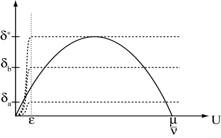
Figure 1. The logistic growth function $U\mapsto U(\mu-\nu U)$ (solid line), and the harvesting function $U\mapsto\delta\rho_{\varepsilon}(U)$ for three values of $\delta$ (dashed lines). The abscissae of the points of intersection of the solid and dashed lines correspond, respectively, to remnant (if smaller than $\varepsilon$) and significant (if strictly larger than $\varepsilon$) stationary solutions of (2.9). We observe that the number of significant solutions is as follows: one if $\delta<k(\varepsilon)$ (case $\delta=\delta_{a}$); two if $k(\varepsilon)\leq\delta<\mu^{2}/(4\nu)$ (case $\delta=\delta_{b}$); one if $\delta=\mu^{2}/(4\nu)$ (case $\delta=\delta^{*}$); zero if $\delta>\mu^{2}/(4\nu)$. The number of nonzero remnant solutions is zero or more if $\delta\leq k(\varepsilon)$ (depending on the shape of $\rho_{\varepsilon}$); one or more if $\delta>k(\varepsilon),$ since, from (2.3), $\rho^{\prime}_{\varepsilon}(0)=0$. We assumed here that $\varepsilon_{0}=\varepsilon$.

Remark 2.1.

The concepts of remnant and significant solutions, as well as the harvesting term $\delta h(x)\rho_{\varepsilon}(u)$, are not classical. In order to clarify these notions, we present in Figure 1 a short graphical study of the nonspatial model

(2.9) $$\frac{dU}{dt}=U(\mu-\nu U)-\delta\rho_{\varepsilon}(U)=:k(U),\quad t\in\mathbb{R}_{+},$$

with constant coefficients $\mu,\nu>0$.

Since $\varepsilon_{0}$ is assumed to be small in our model, the remnant solutions of (2.7) correspond to very low population densities. On the other hand, significant solutions are everywhere above $\varepsilon_{0}$. In particular, a constant yield is ensured in that case. In contrast to the ODE case, stationary solutions which are neither remnant nor significant may exist, as outlined in the next theorems. However, as we will see while studying the long-time behavior of the solutions of the model (2.1), they are of less importance (see Theorem 2.6 and section 3). The threshold $\varepsilon_{0}$ is different from $\varepsilon$ in general. We had to define remnant and significant functions using $\varepsilon_{0}$ for technical reasons (see the proof of Theorem 2.5.ii, equation (2.27)). Since $\varepsilon$ is assumed to be very small, it has no implication on the biological interpretation of our results. Moreover, most of our results still work when $\varepsilon_{0}$ is replaced by $\varepsilon$.

Let us now start our analysis of (2.7). In what follows, we always assume that

(2.10) $$\varepsilon_{0}<\displaystyle{\frac{-\lambda_{1}\underline{\phi}}{4\overline{\nu}}},$$

so that, in particular, from Proposition 2.1, the solution $p_{0}$ of (2.6) is significant.

We begin by proving that there exists a threshold $\delta^{\ast}$ such that, if the amplitude $\delta$ is below $\delta^{\ast}$, (2.7) admits significant solutions, while it does not in the other case.

Theorem 2.3.

Assume that $\lambda_{1}<0;$ then there exists $\delta^{\ast}\geq 0$ such that

(i) if $\delta\leq\delta^{\ast},$ there exists at least a positive significant solution $p_{\delta}\leq p_{0}$ of (2.7);

(ii) if $\delta>\delta^{\ast},$ there is no positive significant solution of (2.7).

Remark 2.2.

There is no positive bounded solution of (2.7) whenever $\lambda_{1}\geq 0$.

Under stronger hypotheses, we are able to prove that (2.7) admits at most two significant solutions. In order to state this result, we need some definitions. Let $G$ be the space defined by

(2.11) $$G:=H^{1}(C)$$

in the bounded case, and by

(2.12) $$G:=H^{1}_{per}=\left\{\psi\ \in\ H^{1}_{loc}(\mathbb{R}^{N})\text{ such that }\psi\text{ is L-periodic}\right\}$$

in the periodic case. Let us define the standard Rayleigh quotient: for all $\psi\in G$, $\psi\not\equiv 0$, and for all $\sigma\in L^{\infty}(C)$,

(2.13) $$\mathcal{R_{\sigma}(\psi)}:=\frac{{\int_{C}}D|\nabla\psi|^{2}-\sigma(x)\psi^{2}}{{\int_{C}}\psi^{2}}.$$

According to the Courant–Fischer theorem (see, e.g., [7]), the second smallest eigenvalue $\lambda_{2}$ of the operator $\mathcal{L}_{\mu}$ can be characterized by

(2.14) $$\lambda_{2}=\min_{E_{k}\subset G,\text{dim}(E_{k})=2}\max_{\psi\in E_{k},\ \psi\not\equiv 0}\mathcal{R_{\mu}}(\psi).$$

This characterization is equivalent to the classical one given in [19].

We are now in position to state the following theorem.

Theorem 2.4.

Assume that $\lambda_{1}<0\leq\lambda_{2};$ then, in the bounded case, (2.7) admits at most two significant solutions. In the periodic case, (2.7) admits at most two L^′-periodic significant solutions for all L${}^{\prime}\in(0,+\infty)^{N}$. Moreover, under these hypotheses, if two solutions $p_{1,\delta}$ and $p_{2,\delta}$ exist, they are ordered in the sense that, for instance, $p_{1,\delta}<p_{2,\delta}$ in $\Omega$.

Remark 2.3.

Similar methods also allow us to assess a result on the number of solutions of (2.8). Indeed, if $\lambda_{1}<0\leq\lambda_{2}$, then we obtain that (2.8) admits at most two nonnegative bounded (and periodic in the periodic case) solutions. If these solutions exist, they are ordered.

In the periodic case, Theorem 2.4 also gives some information on the periodicity of the significant solutions of (2.7), which are actually found to have the same periodicity as the coefficients of (2.7), as seen in the next result.

Corollary 2.1.

Assume that $\lambda_{1}<0\leq\lambda_{2}$. Then, in the periodic case, the significant periodic solutions of (2.7) are L-periodic.

The fact that $\lambda_{1}<0$ is directly related to the instability of the trivial solution in the SKT model. The additional condition $\lambda_{2}\geq 0$ in this theorem is linked to the existence of a stable manifold or center manifold of the steady state 0 of the SKT model, in some appropriate functional spaces (see [40]). Therefore, the assumptions of Theorem 2.4, and the Krein Rutmann theory, allow us to conclude that under these assumptions the unstable manifold of 0 is of dimension equal to one or equivalently the stable manifold is of codimension 1. Such results on multiplicity of solutions of elliptic nonlinear equations with a source or sink term have been investigated in the past and are known nowadays as being of Ambrosetti-problem type. These results also involve manifolds of codimension 1 (in the functional space of forcing) and first and second eigenvalues (for the Laplace operator only) (see [28] for a survey of these results).

In any event, Theorem 2.4 relies on the assumption that $\lambda_{2}\geq 0$. In the next proposition, we give conditions under which $\lambda_{2}$ may become positive.

Proposition 2.2.

(i) In the bounded case, if $C$ is a (smooth) domain with diameter $d:=\max_{x,y\in C}\|x-y\|_{\mathbb{R}^{N}},$ $\lambda_{2}(C)\geq D(\frac{\pi}{d})^{2}-\max_{C}\mu$.

(ii) In the periodic case, $\lambda_{2}(C)\geq D(\frac{\pi}{L_{d}})^{2}-\max_{C}\mu,$ where $L_{d}$ denotes the length of the longest diagonal of the period cell $C$.

For instance, when $C=[0,1]\times[0,1]$, we have $d=L_{d}=\sqrt{2}$; thus, for $D=1$ and $\max_{C}{\mu}=4$, we get $\lambda_{2}>0.9$. However, this lower bound is far from being optimal. Indeed, in all our computations of section 3, and under the same hypothesis on $C$ and $D$, we always had $\lambda_{2}>0$, while $\max_{C}{\mu}=10$. Sharper lower bounds for $\lambda_{2}$ can be found in [12]; however, those bounds are also more sensitive to the geometry of the domain and thus less general. They are therefore not detailed here.

We now introduce a result which is important for more applied ecological questions. Indeed, one of the main drawbacks of Theorem 2.3 is that it gives no computable bound for $\delta^{\ast}$. Obtaining information on the value of $\delta^{\ast}$ is precious for ecological questions such as the study of the relationships between $\delta^{\ast}$ and the environmental heterogeneities. The next theorem states some computable estimates of $\delta^{\ast}$.

Let us define

(2.15) $$\delta_{1}:=\displaystyle{\frac{\lambda_{1}^{2}\underline{\phi}}{\overline{\nu}(1+\underline{\phi})^{2}}}\quad\hbox{and}\quad\delta_{2}:=\displaystyle{\frac{\lambda_{1}^{2}}{4\alpha\underline{\nu}}}.$$

Note that neither $\delta_{1}$ nor $\delta_{2}$ depend on $\delta$ and $\varepsilon$.

Theorem 2.5.

(i) If $\lambda_{1}<0$ and $\delta\leq\delta_{1},$ then there exists a positive significant (and $L$-periodic in the periodic case) solution $p_{\delta}$ of (2.7) such that $p_{\delta}\geq-\frac{\lambda_{1}\phi}{\overline{\nu}(1+\underline{\phi})}$.

(ii) If $\lambda_{1}<0$ and $\delta>\delta_{2},$ the only possible positive bounded solutions of (2.7) are remnant.

The lower bound of part (i), for $p_{\delta}$, does not depend on $\varepsilon$. Thus, there is a clear distinction between the remnant and significant solutions. Note that, of course, $\delta_{1}\leq\delta_{2}$.

The formulae (2.15) allow numerical evaluations. An important quantity to compute is the size of the gap $\delta_{2}-\delta_{1}$ and its fluctuations in terms of environmental configurations. This question is addressed in section 3 through a numerical study.

2.4. Asymptotic behavior

In this section, we prove that the quantity $\delta^{\ast}$ in fact corresponds to a maximum sustainable yield, in the sense that when $\delta$ is smaller than $\delta^{\ast}$, the population density $u(t,x)$ converges to a significant stationary state of (2.1) as $t\to\infty$, whereas when $\delta$ is larger than $\delta^{\ast}$, the population density converges to a stationary state which is not significant. In fact, when $\delta$ is larger than the quantity $\delta_{2}$ defined by (2.15) we even prove that the population converges to a remnant stationary state of (2.1).

We assume here that the harvesting starts on a stabilized population governed by the standard SKT model with $\delta=0$. From Theorem 2.2, this means that we study the behavior of the solutions $u(t,x)$ of our model (2.1), starting with the initial datum $u(0,x)=p_{0}(x)$. Since we have assumed that $\lambda_{1}<0$, it follows from Theorem 2.1, Proposition 2.1, and (2.10) that $p_{0}$ is well defined and significant.

Let us describe, with the next theorem, the long-time behavior of the population density.

Theorem 2.6.

Let $u(t,x)$ be the solution of (2.1) with initial datum $u(0,x)=p_{0}(x)$. Then $u$ is nonincreasing in $t$ and the following hold:

(i) If $\delta\leq\delta^{\ast},$ $u(t,x)\to p_{\delta}(x)$ uniformly in $\Omega$ as $t\to+\infty,$ where $p_{\delta}$ is the maximal significant solution of (2.7). Moreover, $p_{\delta}$ is L-periodic in the periodic case.

(ii) If $\delta>\delta^{\ast},$ then the function $u(t,\cdot)$ converges uniformly in $\Omega$ to a solution of (2.7) which is not significant.

(iii) If $\delta>\delta_{2},$ the function $u(t,\cdot)$ converges uniformly in $\Omega$ to a remnant solution of (2.7).

Remark 2.4.

If, in addition, we assume that $\lambda_{2}\geq 0$, then Theorem 2.4 says that, whenever $\delta\leq\delta^{\ast}$, (2.1) admits at most two significant stationary states (which are periodic stationary states in the periodic case). In that case, the stationary state $p_{\delta}$ selected at large times is the higher one. If we do not assume that $\lambda_{2}\geq 0$, this stationary state can still be defined as “the maximal one” that can be constructed by a sub- and supersolution method (see [4]).

From the above theorem, we observe that, whenever $\delta\leq\delta^{\ast}$, the solution $u(t,x)$ of (2.1), with initial datum $p_{0}$, remains significant for all times $t\geq 0$. This ensures a constant yield in time and justifies the name of the model.

Similar results could be obtained for a wider class of initial data. Indeed, with similar methods, the convergence of $u(t,x)$ to a significant solution of (2.7) can be obtained whenever $\delta\leq\delta^{\ast}$ for all bounded and continuous initial data $u(0,x)$ which are larger than the smallest significant solution of (2.7). In particular, when $u(0,x)$ is larger than the maximal significant solution of (2.7), $u(t,x)$ converges to this maximal significant solution as $t\to+\infty$. A more detailed analysis of the basin of attraction related to the maximal significant solution will be further investigated in the forthcoming paper [14].

Theorem 2.6 shows that the practical determination of $\delta^{*}$ is directly linked to the size of the gap $\delta_{2}-\delta_{1}$. As we will see in section 3, this gap $(\delta_{1},\delta_{2})$ can be very narrow in certain situations. In those cases, the numerical computation of $\delta_{1}$ and $\delta_{2}$ therefore gives a sharp localization of the maximum sustainable quota $\delta^{\ast}\in[\delta_{1},\delta_{2}]$, which can be of nonnegligible ecological interest.

2.5. Proofs of the results of section 2

Proof of Proposition 2.1. Let $\phi$ be defined by (2.5), with the appropriate boundary conditions. Set $\kappa_{0}:=\frac{-\lambda_{1}}{\overline{\nu}}$. Then the function $\kappa_{0}\phi$ satisfies

$$-D\nabla^{2}(\kappa_{0}\phi)-\mu(x)\kappa_{0}\phi+\nu(x)(\kappa_{0}\phi)^{2} = \lambda_{1}\kappa_{0}\phi+\nu(x)(\kappa_{0}\phi)^{2}$$

$$= \kappa_{0}\phi(\lambda_{1}+\nu(x)\kappa_{0}\phi)\leq 0.$$

Thus $\kappa_{0}\phi$ is a subsolution of (2.6) satisfied by $p_{0}$. Since for $M\in\mathbb{R}$ large enough $M$ is a supersolution of (2.6), it follows from the uniqueness of the positive bounded solution $p_{0}$ of (2.6) that $p_{0}\geq\kappa_{0}\phi\geq\frac{-\lambda_{1}\underline{\phi}}{\overline{\nu}}$.   $\Box$

Before proving Theorem 2.3, we begin with the following lemma.

Lemma 2.1.

For all $\delta>0,$ if $p_{\delta}$ is a nonnegative bounded solution of (2.7), then $p_{\delta}\leq p_{0}$.

Proof of Lemma 2.1. Assume that there exists $x_{0}\in\Omega$ such that $p_{\delta}(x_{0})>p_{0}(x_{0})$. The function $p_{\delta}$ satisfies

$$-D\nabla^{2}p_{\delta}-p_{\delta}(\mu(x)-\nu(x)p_{\delta})=-\delta h(x)\rho_{\varepsilon}(p_{\delta})\leq 0,$$

and thus $p_{\delta}$ is a subsolution of (2.6) satisfied by $p_{0}$. Since for $M\in\mathbb{R}$ large enough $M$ is a supersolution of (2.6), we can apply a classic iterative method to infer the existence of a solution $p^{\prime}_{0}$ of (2.6) (with Neumann boundary conditions in the bounded case since both $p_{\delta}$ and $M$ satisfy Neumann boundary conditions) such that $p_{\delta}\leq p^{\prime}_{0}\leq M$. In particular, $p^{\prime}_{0}(x_{0})>p_{0}(x_{0})$, which is in contradiction with the uniqueness of the positive bounded solution of (2.6).   $\Box$

Proof of Theorem 2.3. Let us define

$$\delta^{\ast}:=\sup\{\delta\geq 0,{\rm(\ref{eq_sta_e})}\hbox{ admits a significant solution}\}.$$

For $\delta=0$, we know from Proposition 2.1 that $p_{0}$ is a significant solution of (2.7). Moreover, for $\delta$ large enough, the nonexistence of significant solutions of (2.7) is a direct consequence of the maximum principle (it is also a consequence of the proof of Theorem 2.5.ii). Thus $\delta^{\ast}$ is well defined and bounded.

Assume that $\delta^{\ast}>0$, and let us prove that ($\ref{eq_sta_e},\delta^{\ast}$) admits a significant solution. By definition of $\delta^{\ast}$, there exists a sequence $(p_{\delta_{k}})_{k\in\mathbb{N}}$ of solutions of ($\ref{eq_sta_e},\delta_{k}$) with $0<\delta_{k}\leq\delta^{\ast}$ and $\delta_{k}\to\delta^{\ast}$ as $k\to+\infty$. Moreover, from Lemma 2.1, $\varepsilon_{0}\leq p_{\delta_{k}}\leq p_{0}$ for all $k\geq 0$. Thus, from standard elliptic estimates and Sobolev injections, the sequence $(p_{\delta_{k}})_{k\in\mathbb{N}}$ converges (up to the extraction of some subsequence) in $W^{2,\tau}_{loc}$, for all $1\leq\tau<\infty$, to a significant solution $p_{\delta^{\ast}}$ of ($\ref{eq_sta_e},\delta^{\ast}$).

Now, let $0\leq\delta<\delta^{\ast}$. Then

$$-D\nabla^{2}p_{\delta^{\ast}}-p_{\delta^{\ast}}(\mu(x)-\nu(x)p_{\delta^{\ast}})+\delta h(x)=(\delta-\delta^{\ast})h(x)<0,$$

and thus $p_{\delta^{\ast}}$ is a subsolution of ($\ref{eq_sta_e},\delta$). Since $p_{0}$ is a supersolution of ($\ref{eq_sta_e},\delta$), and $p_{\delta^{*}}\leq p_{0}$, a classical iterative method gives the existence of a significant solution $p_{\delta}$ of ($\ref{eq_sta_e},\delta$) (with Neumann boundary conditions in the bounded case since both $p_{0}$ and $p_{\delta}$ satisfy Neumann boundary conditions). This concludes the proof of Theorem2.3.   $\Box$

Proof of Theorem 2.4. As a preliminary, we prove that if two solutions exist, then they cannot intersect. Let $p_{1,\delta}$ and $p_{2,\delta}$ be two significant solutions of (2.7). In the bounded case, we assume that $p_{1,\delta}$ and $p_{2,\delta}$ satisfy Neumann boundary conditions. In the periodic case, we assume that there exists L${}^{\prime}\in(0,+\infty)^{N}$ such that $p_{1,\delta}$ and $p_{2,\delta}$ are L^′-periodic, and then denote the period cell by $C^{\prime}$. Let us set $q_{\delta}:=p_{2,\delta}-p_{1,\delta}$. Then $q_{\delta}$ verifies

(2.16) $$-D\nabla^{2}q_{\delta}-[\mu(x)-\nu(x)(p_{1,\delta}+p_{2,\delta})]q_{\delta}=0;$$

thus, setting $\rho(x):=\mu(x)-\nu(x)(p_{1,\delta}+p_{2,\delta})$, we obtain

(2.17) $$-D\nabla^{2}q_{\delta}-\rho(x)q_{\delta}=0,$$

with the same boundary conditions that were satisfied by $p_{1,\delta}$ and $p_{2,\delta}$.

Let $\widehat{\lambda_{1}}$ and $\widehat{\lambda_{2}}$ be respectively the first and second eigenvalues of the operator $\mathcal{L}_{\rho}:=-D\nabla^{2}-\rho I$. Let $\mathcal{R}_{\sigma}(\phi)$, be defined by (2.13). Since $\rho(x)<\mu(x)-2\underline{\nu}\varepsilon_{0}$ for all $x\in\Omega$, we get

$$\mathcal{R_{\rho}(\varphi)}\geq\mathcal{R_{\mu}(\varphi)}+2\underline{\nu}\varepsilon_{0}$$

for all $\varphi\in G^{\prime}$, where $G^{\prime}:=H^{1}(C)$ in the bounded case and

$$G^{\prime}:=H^{1}_{per}=\left\{\varphi\ \in\ H^{1}_{loc}(\mathbb{R}^{N})\text{ such that }\varphi\text{ is L}^{\prime}\hbox{-periodic}\right\}$$

in the periodic case. Thus, by the classical min-max formula (2.14), it follows that

(2.18) $$\widehat{\lambda_{2}}\geq\lambda_{2}+2\underline{\nu}\varepsilon_{0}>0.$$

Furthermore, from (2.17), 0 is an eigenvalue of the operator $\mathcal{L}_{\rho}$. Thus, (2.18) implies that $\widehat{\lambda_{1}}=0$. As a consequence, $q_{\delta}$ is a principal eigenfunction of the operator $\mathcal{L}_{\rho}$. The principal eigenfunction characterization thus implies that $q_{\delta}$ has a constant sign. Finally, we get that $p_{1,\delta}$ and $p_{2,\delta}$ do not intersect each other.

Let us now prove that (2.7) admits at most two significant solutions. Arguing by contradiction, we assume that there exist three significant (L^′-periodic in the periodic case, for some L${}^{\prime}\in(0,+\infty)^{N}$) solutions $p_{1,\delta}$, $p_{2,\delta}$, and $p_{3,\delta}$ of (2.7). From the above result, we may assume, without loss of generality, that $p_{3,\delta}>p_{2,\delta}>p_{1,\delta}>\varepsilon_{0}$. Set $q_{2,1}:=p_{2,\delta}-p_{1,\delta}$ and $q_{3,2}:=p_{3,\delta}-p_{2,\delta}$; then these functions satisfy the equations

(2.19) $$-D\nabla^{2}q_{2,1}-\rho_{2,1}(x)q_{2,1}=0$$

and

(2.20) $$-D\nabla^{2}q_{3,2}-\rho_{3,2}(x)q_{3,2}=0,$$

with $\rho_{2,1}:=\mu(x)-\nu(x)(p_{1,\delta}+p_{2,\delta})$ and $\rho_{3,2}:=\mu(x)-\nu(x)(p_{2,\delta}+p_{3,\delta})$. Moreover, $q_{2,1}>0$ and $q_{3,2}>0$. Thus 0 is the first eigenvalue of the operators $\mathcal{L}_{\rho_{2,1}}:=-D\nabla^{2}-\rho_{2,1}I$ and $\mathcal{L}_{\rho_{3,2}}:=-D\nabla^{2}-\rho_{3,2}I$ with either Neumann or L^′-periodic boundary conditions.

From the strong maximum principle (see, e.g., [19]) (together with Hopf’s lemma in the bounded case, and using the L^′-periodicity of $q_{3,2}$ in the periodic case), we obtain the existence of $\theta>0$ such that $q_{3,2}>\theta$. Since the operator $\mathcal{L}_{\rho_{3,2}}$ is self-adjoint, we have the following formula for its first eigenvalue $\widehat{\lambda_{1}}^{3,2}$:

$$\widehat{\lambda_{1}}^{3,2}=\min_{\varphi\in G^{\prime}}\mathcal{R}_{\rho_{3,2}}(\varphi).$$

Thus

$$\widehat{\lambda_{1}}^{3,2}=\min_{\varphi\in G^{\prime}}\left\{\mathcal{R}_{\rho_{2,1}}(\varphi)+\frac{\int_{C}\nu(p_{3,\delta}-p_{1,\delta})\varphi^{2}}{\int_{C}\varphi^{2}}\right\} \geq \min_{\varphi\in G^{\prime}}\left\{\mathcal{R}_{\rho_{2,1}}(\varphi)\right\}+\underline{\nu}\theta$$

$$\geq \widehat{\lambda_{1}}^{2,1}+\underline{\nu}\theta,$$

where $\widehat{\lambda_{1}}^{2,1}$ is the first eigenvalue of the operator $\mathcal{L}_{\rho_{2,1}}$. Since the first eigenvalues of the operators $\mathcal{L}_{\rho_{2,1}}$ and $\mathcal{L}_{\rho_{3,2}}$ are both 0, we deduce that $0\geq 0+\underline{\nu}\theta>0$, hence a contradiction.   $\Box$

Proof of Corollary 2.1. Let $p_{\delta}$ be a significant L^′-periodic solution of (2.7), and let $k\in\prod_{i=1}^{N}L_{i}\mathbb{Z}$. From the L-periodicity of (2.7), $p_{\delta}({\cdot}+k)$ is also a solution of (2.7). By periodicity of $p_{\delta}$, the functions $p_{\delta}$ and $p_{\delta}(\cdot+k)$ intersect each other. Thus, from Theorem 2.4, since $p_{\delta}$ and $p_{\delta}(\cdot+k)$ are both L^′-periodic, $p_{\delta}\equiv p_{\delta}(\cdot+k)$. Therefore, $p_{\delta}$ is an L-periodic function.   $\Box$

Proof of Proposition 2.2. In the bounded case, let $\tilde{C}$ be the convex hull of the set $C$. It was proved in [31] that the second Neumann eigenvalue of the Laplace operator $-D\nabla^{2}$ on $\tilde{C}$ was larger than $D(\frac{\pi}{d})^{2}$. Since $C\subset\tilde{C}$, we have $H^{1}(C)\subset H^{1}(\tilde{C})$. Using formula (2.14), we thus obtain that the second eigenvalue of $\mathcal{L}_{\mu}$ in the bounded case satisfies $\lambda_{2}\geq D(\frac{\pi}{d})^{2}-\max_{C}\mu$. This proves part (i) of Proposition 2.2.

In the periodic case, since $H^{1}_{per}$ can be seen as a subset of $H^{1}(C)$, it follows from (2.14) that

(2.21) $$\lambda_{2}\geq\min_{E_{k}\subset H^{1}(C),\text{dim}(E_{k})=2}\max_{\psi\in E_{k},\ \psi\not\equiv 0}\mathcal{R_{\mu}}(\psi).$$

The period cell $C$ is convex but not smooth enough to assert that the right-hand side of (2.21) is equal to the second eigenvalue in the bounded case. Let $L_{d}$ be the longest diagonal of $C$. Then $C$ is included in a ball $B_{L_{d}}$ of diameter $L_{d}$. Thus, from formula (2.14), the right-hand side of (2.21) is larger than the second eigenvalue of $\mathcal{L}_{\mu}$ on $B_{L_{d}}$. From (i), the conclusion of (ii) follows.   $\Box$

Proof of Theorem 2.5, part (i). Let $\lambda_{1}$ and $\phi$ be defined by (2.5), and let $\kappa$ be a nonnegative real number such that $\kappa>\varepsilon_{0}$. Then we have

(2.22) $$\begin{array}[]{r@{\,}c@{\,}l@{}}-D\nabla^{2}(\kappa\phi)-\kappa\phi(\mu(x)-\kappa\phi\nu(x))+\delta h(x)\rho_{\varepsilon}(\kappa\phi)&\leq&\lambda_{1}\kappa\phi+\kappa^{2}\phi^{2}\nu(x)+\delta\\ &\leq&\kappa\phi(\lambda_{1}+\kappa\phi\nu(x))+\delta\\ &\leq&\displaystyle{\max_{\tau\in I}\{\tau(\lambda_{1}+\tau\overline{\nu})\}+\delta},\end{array}$$

where $I=\{\kappa\phi(x)$, $x\in C\}$. Setting $g(\tau):=\tau(\lambda_{1}+\tau\overline{\nu})$, since $\|\phi\|_{\infty}=1$, and since $g$ is a convex function, it follows from (2.22) that

(2.23) $$-D\nabla^{2}(\kappa\phi)-\kappa\phi(\mu(x)-\kappa\phi\nu(x))+\delta h(x)\rho_{\varepsilon}(\kappa\phi)\leq\max\{g(\kappa),g(\kappa\underline{\phi})\}+\delta.$$

Let us take $\kappa_{0}$ be such that $g(\kappa_{0})=g(\kappa_{0}\underline{\phi})$, namely $\kappa_{0}=-\frac{\lambda_{1}}{\overline{\nu}(1+\underline{\phi})}$ (note that $\kappa_{0}\phi>\varepsilon$). We get

(2.24) $$-D\nabla^{2}(\kappa_{0}\phi)-\kappa_{0}\phi(\mu(x)-\kappa_{0}\phi\nu(x))+\delta h(x)\leq\displaystyle{-\frac{\lambda_{1}^{2}\underline{\phi}}{\underline{\nu}(1+\underline{\phi})^{2}}}+\delta\leq 0,$$

from the hypothesis on $\delta$ of Theorem 2.5.i. Therefore, $\kappa_{0}\phi$ is a subsolution of (2.7) with either L-periodic or Neumann boundary conditions. Moreover, if $M$ is a large enough constant, $M$ is a supersolution of (2.7) with L-periodic or Neumann boundary conditions. Thus, it follows from a classical iterative method that there exists a solution $\underline{p_{\delta}}$ of (2.7), with the required boundary conditions, and which satisfies $\kappa_{0}\phi\leq\underline{p_{\delta}}\leq M$ in $\Omega$. Moreover, in the periodic case, since $\kappa_{0}\phi$ and $M$ are L-periodic and since (2.7) is also L-periodic, it follows that $p_{\delta}$ is L-periodic. Theorem 2.5.i isproved.   $\Box$

Proof of Theorem 2.5, part (ii). Assume that $\lambda_{1}<0$, $\delta>\delta_{2}$, and that there exists a positive bounded solution $p_{\delta}$ of (2.7) which is not remnant; i.e.,

(2.25) $$\exists\ x_{0}\ \text{with}\ p_{\delta}(x_{0})\geq\varepsilon_{0}.$$

Since $\phi$ is bounded from below away from 0 and $p_{\delta}$ is bounded, we can define

(2.26) $$\gamma^{*}=\inf\left\{\gamma>0,\ \gamma\phi>p_{\delta}\text{ in }\Omega\right\}>0.$$

It follows from the definition of $\gamma^{*}$ that $\gamma^{*}\phi\geq p_{\delta}$ in $\Omega$, and in particular, $\gamma^{*}\phi(x_{0})\geq p_{\delta}(x_{0})\geq\varepsilon_{0}$. Since $\|\phi\|_{\infty}=1$, we get $\gamma^{*}\geq\varepsilon_{0}$. Thus,

(2.27) $$\gamma^{*}\phi\geq\varepsilon_{0}\underline{\phi}=\varepsilon,$$

which implies $\rho_{\varepsilon}(\gamma^{*}\phi)=1$. Thus, $h(x)\rho_{\varepsilon}(\gamma^{*}\phi)\geq\alpha$, and we get

$$-D\nabla^{2}(\gamma^{*}\phi)-\gamma^{*}\phi(\mu(x)-\gamma^{*}\phi\nu(x))+\delta h(x)\rho_{\varepsilon}(\gamma^{*}\phi)\geq\gamma^{*}\phi(\lambda_{1}+\gamma^{*}\phi\nu(x))+\delta\alpha$$

on $\Omega$. Moreover, since $\gamma^{*}\phi>0$ and $\nu\geq\underline{\nu}$, we have $\gamma^{*}\phi(\lambda_{1}+\gamma^{*}\phi\nu(x))\geq-\smash{\frac{\lambda_{1}^{2}}{4\underline{\nu}}}$. Using the fact that $\delta>\delta_{2}=\frac{\lambda_{1}^{2}}{4\alpha\underline{\nu}}$, we thus get

(2.28) $$-D\nabla^{2}(\gamma^{*}\phi)-\gamma^{*}\phi(\mu(x)-\gamma^{*}\phi\nu(x))+\delta h(x)\rho_{\varepsilon}(\gamma^{*}\phi)\geq\displaystyle{-\frac{\lambda_{1}^{2}}{4\underline{\nu}}+\delta\alpha}>0$$

on $\Omega$. Therefore, $\gamma^{*}\phi$ is a supersolution of (2.7). Set $z:=\gamma^{*}\phi-p_{\delta}$. From the definition of $\gamma^{*}$, we know that $z\geq 0$ and that there exists a sequence $(x_{n})_{n\in\mathbb{N}}$ in $\Omega$ such that $z(x_{n})\to 0$ as $n\to+\infty$.

In the bounded case, up to the extraction of some subsequence, $x_{n}\to\overline{x}\in\Omega$ as $n\to+\infty$. By continuity, $z(\overline{x})=0$. Moreover, subtracting (2.7) from (2.28), we get

(2.29) $$-D\nabla^{2}z+[\nu(x)(\gamma^{*}\phi+p_{\delta})+\chi(x)-\mu(x)]z>0\quad\text{in }\Omega,$$

where the function $\chi$ is defined by $\chi(x)=\delta h(x)\frac{\rho_{\varepsilon}(\gamma^{*}\phi(x))-\rho_{\varepsilon}(p_{\delta}(x))}{\gamma^{*}\phi(x)-p_{\delta}(x)}$ whenever $\gamma^{*}\phi(x)-p_{\delta}(x)\neq 0$, and $\chi(x)=\rho_{\varepsilon}^{\prime}(p_{\delta}(x))$ otherwise. Since $\rho_{\varepsilon}$ is $C^{1}$, $\chi$ is bounded. Thus $b(x):=\nu(x)(\gamma^{*}\phi+p_{\delta})+\chi(x)-\mu(x)$ is a bounded function. Using the strong elliptic maximum principle, we deduce from (2.29) that $z\equiv 0$. Thus $\gamma^{*}\phi\equiv p_{\delta}$ is a positive solution of (2.7). It is in contradiction with (2.28).

In the periodic case, we must also consider the situation where the sequence $(x_{n})_{n\in\mathbb{N}}$ is not bounded. Let $(\overline{x}_{n})\in\overline{C}$ be such that $x_{n}-\overline{x}_{n}\in\prod_{i=1}^{N}L_{i}\mathbb{Z}$. Up to the extraction of some subsequence, we can assume that there exists $\overline{x}_{\infty}\in\overline{C}$ such that $\overline{x}_{n}\to\overline{x}_{\infty}$ as $n\to+\infty$. Set $\phi_{n}(x)=\phi(x+x_{n})$ and $p_{\delta,n}(x)=p_{\delta}(x+x_{n})$. From standard elliptic estimates and Sobolev injections, it follows that (up to the extraction of some subsequence) $p_{\delta,n}$ converge in $W^{2,\tau}_{loc}$, for all $1\leq\tau<\infty$, to a function $p_{\delta,\infty}$ satisfying

$$-\nabla^{2}(Dp_{\delta,\infty})-p_{\delta,\infty}(\mu(x+\overline{x}_{\infty})-p_{\delta,\infty}\nu(x+\overline{x}_{\infty}))+\delta h(x+\overline{x}_{\infty})\rho_{\varepsilon}(p_{\delta,\infty})=0$$

in $\mathbb{R}^{N}$, while $\gamma^{*}\phi_{n}$ converges to $\gamma^{*}\phi_{\infty}:=\gamma^{*}\phi(\cdot+\overline{x}_{\infty})$, and

$$-\nabla^{2}(D\gamma^{*}\phi_{\infty})-\gamma^{*}\phi_{\infty}(\mu(x+\overline{x}_{\infty})-\gamma^{*}\phi_{\infty}\nu(x+\overline{x}_{\infty}))+\delta h(x+\overline{x}_{\infty})\rho_{\varepsilon}(\gamma^{*}\phi_{\infty})>0$$

in $\mathbb{R}^{N}$. Let us set $z_{\infty}(x):=\gamma^{*}\phi_{\infty}(x)-p_{\delta,\infty}(x)$. Then $z_{\infty}(x)=\lim_{n\to+\infty}z(x+x_{n})$, and therefore $z_{\infty}\geq 0$ and $z_{\infty}(0)=0$. Moreover, there exists a bounded function $b_{\infty}$ such that

(2.30) $$-D\nabla^{2}z_{\infty}+b_{\infty}z_{\infty}>0\quad\hbox{in }\mathbb{R}^{N}.$$

It then follows from the strong maximum principle that $z_{\infty}\equiv 0$, and we again obtain a contradiction. Finally, we necessarily have $p_{\delta}\leq\varepsilon_{0}$, and the proof of Theorem 2.5.ii is complete.   $\Box$

Proof of Theorem 2.6, part (i). Assume that $\delta\leq\delta^{\ast}$. Let $p_{\delta}$ be the unique maximal significant solution defined in the proof of Theorem 2.5.i. Then, from Lemma 2.1,

(2.31) $$p_{\delta}(x)\leq p_{0}(x)=u(0,x)\quad\forall x\in\Omega,$$

which implies

(2.32) $$p_{\delta}(x)\leq u(t,x)\quad\text{in }\mathbb{R}_{+}\times\Omega,$$

since $p_{\delta}$ is a stationary solution of (2.1). Moreover, since $p_{0}$ is a supersolution of (2.7), $u$ is nonincreasing in time $t$, and standard parabolic estimates imply that $u$ converges in $W_{loc}^{2,\tau}\left(\Omega\right)$, for all $1\leq\tau<\infty$, to a bounded stationary solution $u_{\infty}$ of (2.1). Furthermore, from (2.32) we deduce that $p_{\delta}\leq u_{\infty}\leq p_{0}$. Since $p_{\delta}$ is the maximal positive solution of (2.7), it follows that $u_{\infty}\equiv p_{\delta}$. Moreover, in the periodic case, since $p_{0}$ and (2.1) are L-periodic, $u(t,x)$ is also L-periodic in $x$. Therefore the convergence is uniform in $\Omega$. Part (i) of Theorem 2.6 is proved.   $\Box$

Proof of Theorem 2.6, parts (ii) and (iii). Assume that $\delta>\delta^{\ast}$. Since 0 is a stationary solution of (2.1) and $u(0,x)=p_{0}>0$, we obtain that $u(t,x)>0$ in $\mathbb{R}^{+}\times\Omega$, and again, from standard parabolic estimates, we know that $u$ converges in $W_{loc}^{2,\tau}\left(\Omega\right)$ (for all $1\leq\tau<\infty$) to a bounded stationary solution $\underline{u_{\infty}}\geq 0$ of (2.1) as $t\to+\infty$. Moreover, in the periodic case, from the L-periodicity of the initial data and of (2.1), we know that $u(t,\cdot)$ and $\underline{u_{\infty}}$ are L-periodic. Therefore the convergence is uniform in $\Omega$. It follows from Theorem 2.3.ii that $\underline{u_{\infty}}$ cannot be a significant solution of (2.7). Moreover, if $\delta>\delta_{2}$, Theorem 2.5.ii ensures that $\underline{u_{\infty}}$ is a remnant solution of (2.7).    $\Box$

3. Numerical investigation of the effects of environmental fragmentation

We propose here to apply the results of section 2, on the estimation of the maximum sustainable yield, to the study of the effects of environmental fragmentation. A theoretical investigation of the relationships between maximum sustainable yield and fragmentation is difficult to achieve (see Remark 3.1). To overcome this difficulty, we propose a numerical study in the case of stochastic environments. First, we show that the gap $\delta_{2}-\delta_{1}$, obtained from (2.15) and Theorem 2.5, remains small whatever the degree of fragmentation is. This gap corresponds to the numerical values of the harvesting quota $\delta$ for which we do not know whether the population density will converge to a significant or a remnant solution of the stationary equation (2.7). Second, we show that there is a monotone increasing relationship between the maximal sustainable yield $\delta^{\ast}$ and the habitat aggregation.

Remark 3.1.

In a periodic environment, a simple way of changing the degree of fragmentation without changing the relative spatial pattern (favorable area/unfavorable area ratio) is to modify the size of the period cell $C$. Assume that $\mu(x)=\eta(\frac{x}{L})$, for some $1$-periodic function $\eta$ with positive integral and for some $L>0$. This means that the environment consists of square cells of side $L$. Setting $\lambda_{1,L}:=\lambda_{1}$ and $\phi_{L}:=\phi$, we then have $-D\Delta\phi_{L}-\eta\left(\frac{x}{L}\right)\phi_{L}=\lambda_{1,L}\phi_{L}$ on $[0,L]^{N}$. The function $\psi_{L}(x):=\phi_{L}(Lx)$ thus satisfies $-D\Delta\psi_{L}-L^{2}\eta(x)\psi_{L}=L^{2}\lambda_{1,L}\psi_{L}$ in $[0,1]^{N}$, with 1-periodicity. From the Rayleigh formula we thus obtain

$$\lambda_{1,L}=\min_{\psi\in H^{1}_{per}}\frac{D}{L^{2}}\frac{\int_{[0,1]^{N}}|\nabla\psi|^{2}}{\int_{[0,1]^{N}}\psi^{2}}-\frac{\int_{[0,1]^{N}}\eta\psi^{2}}{\int_{[0,1]^{N}}\psi^{2}};$$

therefore $\lambda_{1,L}<0$ (since $\psi\equiv 1\in H^{1}_{per}$), and $\lambda_{1,L}$ decreases with $L$. It implies that $\delta_{2}$ increases with $L$. The relationship between $\delta_{1}$ and $L$ is less clear since $\displaystyle\underline{\phi_{L}}=\min\nolimits_{C}\phi_{L}$ may not always be an increasing function of $L$.

In order to lessen the boundary effects and to focus on fragmentation, we place ourselves in the periodic case. For our numerical computations, we assume that the environment is made of two components, favorable and unfavorable regions. This is expressed in the model (2.1) through the coefficient $\mu(x)$, which takes two values $\mu^{+}$ or $\mu^{-}$, depending on the space variable $x$. We also assume that

$$\mu^{+}>\mu^{-},\quad\nu(x)\equiv 1,\quad h(x)\equiv 1,\hbox{ and }D=1.$$

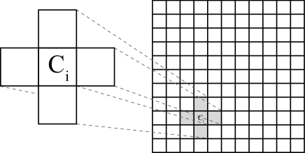
Figure 2. The 4-neighborhood system: an element $C_{i}$ of $C$ and its four neighbors.

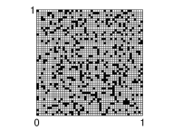
(a) $s=3400$

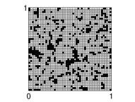
(b) $s=3800$

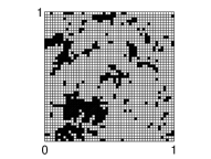
(c) $s=4200$

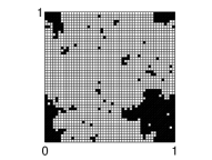
(d) $s=4600$

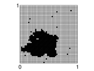
(e) $s=4800$

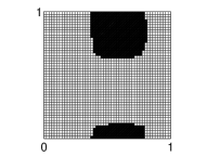
(f) $s=4900$

Figure 3. Some samples of the landscapes used for the computations of $\delta_{1}$ and $\delta_{2},$ with different values of the habitat aggregation index $s$. The black areas correspond to more favorable environment, where $\mu(x)=\mu^{+}$.

Using a stochastic model for landscape generation [35], we built 2000 samples of binary environments, on the two-dimensional period cell $C=[0,1]^{2}$, with different degrees of fragmentation. In all these environments, the favorable region, where $\mu(x)=\mu^{+}$, occupies 20% of the period cell. The environmental fragmentation is defined as follows. We discretize the cell $C$ into $n_{C}=50\times 50$ equal squares $C_{i}$. The lattice made of the cells $C_{i}$ is equipped with a 4-neighborhood system $V(C_{i})$ (see Figure 2), with toric conditions. On each cell $C_{i}$, we assume that the function $\mu$ takes either the value $\mu^{+}$ or $\mu^{-}$, while the number $n_{+}=\hbox{card}\{i$, $\mu\equiv\mu^{+}$ on $C_{i}\}$ is fixed to $n_{C}\times\frac{20}{100}=500$. For each landscape sample $\omega=(\mu(C_{i}))_{i=1,\ldots,n_{C}}$, we set $s(\omega)=\frac{1}{2}\sum_{C_{i}\subset C}\sum_{C_{j}\in V(C_{i})}1\!\!1\{\mu(C_{j})=\mu(C_{i})\}$, the number of pairs of neighbors $(C_{i},C_{j})$ such that $\mu$ takes the same value on $C_{i}$ and $C_{j}$ ($1\!\!1\{\cdot\}$ is the indicator function). The number $s(\omega)$ is directly linked to the environmental fragmentation: a landscape pattern is all the more aggregated as $s(\omega)$ is high, and all the more fragmented as $s(\omega)$ is small (Figure 3). Thus, we shall refer to $s$ as the “habitat aggregation index.”

Remark 3.2.

There exist several ways of obtaining hypothetical landscape distributions. The commonest are neutral landscape models, originally introduced by Gardner et al. [17]. They can include parameters which regulate the fragmentation [21]. We preferred to use a stochastic landscape model presented in [35], since it allows an exact control of the favorable and unfavorable surfaces and is therefore well adapted for analyzing the effects of fragmentation per se. This model is inspired from statistical physics. The number of pairs of similar neighbors $s$ is controlled during the process of landscape generation. This quantity can be measured a posteriori on the landscape samples. Other measures of fragmentation could have been used, such as fractal dimension (see [25]). For a discussion on the different ways of measuring habitat fragmentation in real-world situations, the interested reader can refer to [15].

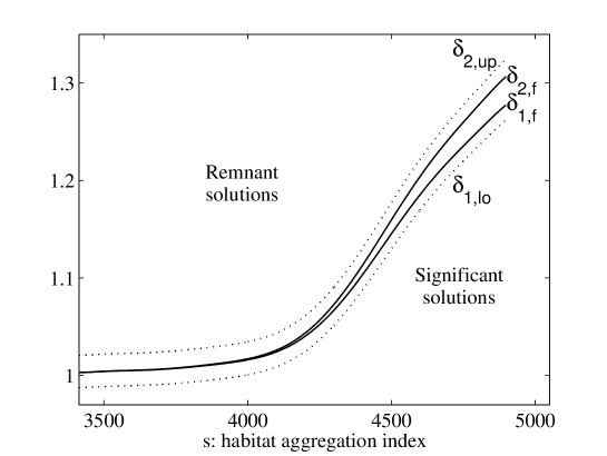
Figure 4. Solid lines: $\delta_{1,f}$ and $\delta_{2,f}$ correspond respectively to the data sets $\{(s^{i},\delta_{1}^{i})\}_{i=1,\ldots,2000}$ and $\{(s^{i},\delta_{2}^{i})\}_{i=1,\ldots,2000},$ fitted with ninth degree polynomials. Dashed lines: $\delta_{1,lo}$ is a lower prediction bound for new observations of $\delta_{1},$ and $\delta_{2,up}$ an upper prediction bound for new observations of $\delta_{2},$ with in both cases a certainty level of 99%.

For our computations, we took $\mu^{+}=10$ and $\mu^{-}=0$, and we computed the corresponding values of $\lambda_{1}^{i}$, $\delta_{1}^{i}$, and $\delta_{2}^{i}$ on each landscape sample $\omega^{i}$ of aggregation index $s^{i}$, for $i=1,\ldots,2000$. The eigenvalues $\lambda_{1}^{i}$ were computed with a finite elements method. We fitted the data sets $\{(s^{i},\delta_{1}^{i})\}_{i=1,\ldots,2000}$ and $\{(s^{i},\delta_{2}^{i})\}_{i=1,\ldots,2000}$ using ninth degree polynomials (it is enough to assess whether the relations between $s$ and $\delta_{1},\delta_{2}$ tend to be monotonic or not). The resulting fitted curves $\delta_{1,f}$ and $\delta_{2,f}$ are presented in Figure 4. Under the assumption of normally distributed values of $\delta_{1}$ and $\delta_{2}$ for fixed $s$ values, we computed a lower prediction bound ($\delta_{1,lo}$) for new observation of $\delta_{1}$ and an upper prediction bound for $\delta_{2}$ ($\delta_{2,up}$), with a level of certainty of 99%. Thus, given a configuration $\omega$, with a fixed value of $s$, when $\delta$ is smaller than $\delta_{1,lo}$ we take a 0.5% chance of being above $\delta_{1}$, while when $\delta$ is larger than $\delta_{2,up}$ we take a 0.5% chance of being below $\delta_{2}$. The small thickness of the intervals $(\delta_{1,lo},\delta_{2,up})$ emphasizes the quality of the relationship between the habitat aggregation index $s$ and the maximum sustainable yield $\delta^{\ast}\in[\delta_{1},\delta_{2}]$. This also indicates that the criteria of Theorems 2.5 and 2.6 are close to being optimal, at least in some situations.

Furthermore, as we can observe, the values of $\delta_{1}$ and $\delta_{2}$ tend to increase as $s$ increases, and thus as the environment aggregates. Since $\delta^{\ast}\in[\delta_{1},\delta_{2}]$, we deduce from the computations presented in Figure 4 that $\delta^{\ast}$ tends to increase with environmental aggregation.

These tests were performed for particular values of $\mu^{+}$ and $\mu^{-}$. However, the thickness of the interval $(\delta_{1},\delta_{2})$ can be determined for all values of $\mu^{+},\mu^{-}$ without further numerical computations, provided that $\mu^{+}-\mu^{-}=10$. Indeed, let us set $B:=\mu^{+}-\mu^{-}$. For a fixed value of $B$, let $\mu_{0}(x)$ be a given L-periodic function in $L^{\infty}(\mathbb{R}^{N})$ taking only the two values $\mu_{0}^{+}=B$ and $\mu_{0}^{-}=0$. Let $\lambda_{1,0}$ be the first eigenvalue of the operator $-\nabla^{2}-\mu_{0}I$ on $C$, with L-periodicity conditions, $\phi_{0}$ the associated eigenfunction with minimal value $\underline{\phi_{0}}$, and

$$\delta_{1,0}:=\displaystyle{\frac{\lambda_{1,0}^{2}\underline{\phi_{0}}}{(1+\underline{\phi_{0}})^{2}}}\quad\hbox{and}\quad\delta_{2,0}:=\displaystyle{\frac{\lambda_{1,0}^{2}}{4}}.$$

We have the following proposition.

Proposition 3.1.

Assume that $\mu(x)=\mu_{0}(x)+\mu^{-},$ with $\mu^{-}>\lambda_{1,0}$. Let $\delta_{1}$ and $\delta_{2}$ be defined by (2.15). Then we have $\delta_{2}-\delta_{1}=(1-\frac{\mu^{-}}{\lambda_{1,0}})^{2}(\delta_{2,0}-\delta_{1,0})$.

This result also indicates that the information on $\delta^{\ast}$ is all the more precise as the growth rate function takes low values. However, the “relative thickness” of the interval $(\delta_{1},\delta_{2})$, compared to $\delta_{1},\frac{\delta_{2}-\delta_{1}}{\delta_{1}}$, does not depend on $\mu^{-}$, as can be easily seen.

Proof of Proposition 3.1. The relation $\lambda_{1}[\mu(x)]=\lambda_{1,0}-\mu^{-}$ is a direct consequence of the uniqueness of the first eigenvalue $\lambda_{1}$. We assume that $\mu^{-}>\lambda_{1,0}$, so that $\lambda_{1}[\mu(x)]<0$. From the uniqueness of the eigenfunction $\phi$ associated with $\lambda_{1}$, $\phi$ does not depend on $\mu^{-}$. Therefore, $\delta_{1}$ and $\delta_{2}$ satisfy $\delta_{1}=\frac{(\lambda_{1,0}-\mu^{-})^{2}\underline{\phi_{0}}}{(1+\underline{\phi_{0}})^{2}}$ and $\delta_{2}=\frac{(\lambda_{1,0}-\mu^{-})^{2}}{4}$. The result immediately follows.   $\Box$

4. A few comments on the proportional harvesting model

In this model, the population density $u$ is governed by the equation

(4.1) $$u_{t}=D\nabla^{2}u+u(\mu(x)-\nu(x)u)-q(x)u,\quad x\in\Omega,$$

with L-periodicity of the functions $\mu(x)$, $\nu(x)$, and $q(x)$ in the periodic case, and with Neumann or Dirichlet boundary conditions in the bounded case. Setting

$$\tau(x):=\mu(x)-q(x),$$

this model becomes equivalent to the SKT model (1.3). Hence, many properties of the solutions of this model are described in the existing literature. In particular the existence, nonexistence, and uniqueness results of Theorems 2.1 and 2.2 apply. The condition $\lambda_{1}[\mu(x)-q(x)]<0$ is therefore necessary and sufficient for species persistence. Furthermore, the theoretical results of [9], [13], [34], [35] on the effects of habitat arrangement on species persistence are also true for this model.

For instance, when the function $\mu(x)$ is constant, with $\mu(x)\equiv\mu_{1}>0$, and if the domain $\Omega$ is convex and symmetric with respect to each axis $\{x_{1}=0\},\ldots,\{x_{N}=0\}$, the next result is a straightforward consequence of the paper [9].

Theorem 4.1.

(i) In the periodic case, $\lambda_{1}[\mu_{1}-q_{k}^{*}(x)]\leq\lambda_{1}[\mu_{1}-q(x)]$.

(ii) In the bounded Dirichlet case, $\lambda_{1}[\mu_{1}-q_{k}^{*}(x)]\leq\lambda_{1}[\mu_{1}-q(x)]$.

(iii) In the bounded Neumann case, if $\Omega$ is a rectangle, $\lambda_{1}[\mu_{1}-q_{k}^{\sharp}(x)]\leq\lambda_{1}[\mu_{1}-q(x)]$.

Here $q_{k}^{*}$ denotes the symmetric decreasing Steiner rearrangement of the function $q$ with respect to the variable $x_{k}$, and $q_{k}^{\sharp}$ denotes the monotone rearrangement of $q$ with respect to $x_{k}$ (see [9] and [11] for the definition of these rearrangements). These rearrangements of a function $q$ preserve not only its mean value, but also its distribution function. This means that if, for instance, $q$ corresponds to a “patch” function taking the values $q_{1}$, $q_{2}$, and $q_{3}$ in some regions $A_{1}$, $A_{2}$, and $A_{3}$, respectively, with $A_{1}+A_{2}+A_{3}=|C|$, then the areas of the regions where the rearranged functions $q^{*}$ and $q^{\sharp}$ take the values $q_{1}$, $q_{2}$, and $q_{3}$ remain equal to $A_{1}$, $A_{2}$, and $A_{3}$, respectively.

Theorem 4.1 combined with Theorem 2.2 says that the spatially rearranged harvesting strategies are better for species survival. This result can be helpful from a resource management point of view. Indeed, the authorities can rearrange the position of the harvested areas in order to improve the chances of population persistence. The result of Theorem 4.1 shows that, in the framework of these models, the creation of a large reserve gives persistence more chances than the creation of several small reserves, and is in accordance with the former results of [24] and [27] in the Dirichlet case. See Figure 5 for some illustrations in the bounded case with Dirichlet and Neumann boundary conditions.

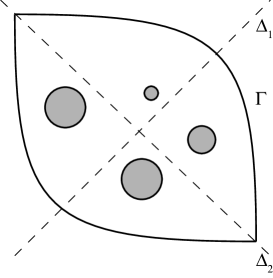
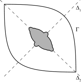
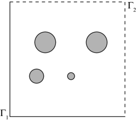
Figure 5. Examples of applications of Theorem 4.1.ii–iii to reserves management. In panels (a) and (b), the boundary $\Gamma$ of $\Omega$ is lethal (Dirichlet boundary conditions). (a) The initial effort function $q(x)$ takes two values, $q^{+}>0$ in the white area, and $q^{-}=0$ in the shadowed regions, which correspond to reserves. (b) Position of the reserves after a symmetric decreasing Steiner rearrangement along the $\Delta_{1}$ and $\Delta_{2}$ axes, successively. The rearranged configuration (b) always give more chances of species persistence. In panels (c) and (d), the boundary $\Gamma$ is divided into two parts: $\Gamma=\Gamma_{1}\cup\Gamma_{2}$. $\Gamma_{1}$ is represented with a solid line and can correspond to a coast, while $\Gamma_{2}$ is represented with a dashed line and can correspond to a nonphysical limit that the species cannot cross (Neumann boundary conditions). (c) The effort function $q(x)$ again takes two values, $q^{+}>0$ in the white area, and $q^{-}=0$ in the reserves. (d) Position of the reserves after monotone rearrangement along the horizontal and vertical axes, successively. The chances of persistence are better in the rearranged configuration (d).

5. Discussion

We have proposed a model for the study of populations in heterogeneous environments, for populations submitted to an external negative forcing term. This forcing term could be regarded as a “quasi-constant-yield” harvesting, depending only on the population density $u$ when $u$ is below a certain small threshold $\varepsilon$. The introduction of such a threshold $\varepsilon$ was necessary for ensuring the nonnegativity of the solutions of our model, and therefore its actuality.

We carried out new mathematical results on the elliptic equation satisfied by the stationary states of the model, and on the associated parabolic equation. Both qualitative and quantitative results were obtained.

From the qualitative point of view, we described the behavior of the model solutions in terms of the harvesting amplitude $\delta$. Two main types of stationary solutions were found: the remnant solutions, always below a small threshold $\varepsilon_{0}$ and therefore close to 0, and the significant solutions, always above this threshold, thus ensuring a time-constant yield. We discussed the maximum number of significant stationary solutions, which we found equal to 2, under a hypothesis of positivity of the second eigenvalue $\lambda_{2}$ of a linear operator. We further investigated the long-time behavior of the solution of our model, starting from a nonharvested population at equilibrium. We found a critical value $\delta^{*}$ of the harvesting term amplitude, below which the population density tends over time to a significant stationary solution, and above which it converges to a stationary solution which is not significant. We also established quantitative formulae for some lower and upper bounds for $\delta^{*}$: $\delta_{1}$ and $\delta_{2}$, respectively. The threshold $\delta_{2}$ has the additional property that, whenever the amplitude $\delta$ is above $\delta_{2}$, the population density decreases to a remnant stationary solution.

The quantitative aspects of our study mainly consisted of discussing the effect of environmental fragmentation on these thresholds $\delta_{1}$ and $\delta_{2}$, and therefore on the interactions between environmental fragmentation and maximum sustainable yield. Namely, when computing the values of $\delta_{1}$ and $\delta_{2}$ on 2000 samples of stochastically obtained patchy environments, with different levels of fragmentation, we found an increasing relationship between these two coefficients and an environmental aggregation index $s$. This indicates that, for given areas of favorable and unfavorable regions, the harvesting quota that a species can sustain, while ensuring a time-constant yield, is higher when the favorable regions are aggregated.

The reader may note that, in our model, the species mobility was not affected by the environmental heterogeneity. Such a dependence could be modeled by using a more general dispersion term, of the form $\nabla\cdot(A(x)\nabla u)$, instead of $D\nabla^{2}u$, where $A(x)$ stands for the diffusion matrix (see [9], [37]). In fact, most of our results still work when the matrix $A$ is of class $C^{1,\alpha}$ (with $\alpha>0$) and uniformly elliptic, i.e., when there exists $\tau>0$ such that $A(x)\geq\tau I_{N}$ for all $x\in\Omega$. Indeed, Theorems 2.1, 2.2, 2.4, 2.5, and 2.6 remain true under this more general assumption. However, the effects of environmental heterogeneity may differ, depending on the way $A(x)$ and $\mu(x)$ are correlated (see [22]). In the proportional harvesting case, the results of section 4 on the effects of the arrangements of the harvested regions may also not be valid with this dispersion term. However, in situations where $A(x)$ takes low values (slow motion) when $q(x)$ is low (“reserves”; see section 4), as underlined in [34], a simultaneous rearrangement of the functions $A(x)$ and $q(x)$ would lead to lower $\lambda_{1}$ values and therefore to higher chances of species survival.

References

- [1]
- [2] R. A. Adams, Sobolev Spaces, Academic Press, New York, 1975.
- [3] H. Amann, Fixed point equations and nonlinear eigenvalue problems in ordered Banach spaces, SIAM Rev., 18 (1976), pp. 620–709.
- [4] H. Amann, Supersolution, monotone iteration and stability, J. Differential Equations, 21 (1976), pp. 367–377.
- [5] J. E. M. Baillie, C. Hilton-Taylor, and S. N. Stuart, eds., 2004 IUCN Red List of Threatened Species. A Global Species Assessment, IUCN, Gland, Switzerland, Cambridge, UK, 2004.
- [6] J. R. Beddington and R. M. May, Harvesting natural populations in a randomly fluctuating environment, Science, 197 (1977), pp. 463–465.
- [7] Z. Belhachmi, D. Bucur, G. Buttazzo, and J.-M. Sac-Epée, Shape optimization problems for eigenvalues of elliptic operators, ZAMM Z. Angew. Math. Mech., 86 (2006), pp. 171–184.
- [8] H. Berestycki and F. Hamel, Front propagation in periodic excitable media, Comm. Pure Appl. Math., 55 (2002), pp. 949–1032.
- [9] H. Berestycki, F. Hamel, and L. Roques, Analysis of the periodically fragmented environment model: I—Species persistence, J. Math. Biol., 51 (2005), pp. 75–113.
- [10] H. Berestycki, F. Hamel, and L. Roques, Analysis of the periodically fragmented environment model: II—Biological invasions and pulsating travelling fronts, J. Math. Pures Appl., 84 (2005), pp. 1101–1146.
- [11] H. Berestycki and T. Lachand-Robert, On the monotone rearrangement in cylinders and applications, Math. Nachr., 266 (2004), pp. 3–19.
- [12] J. H. Bramble and L. E. Payne, Bounds in the Neumann problem for second order uniformly elliptic operators, Pacific J. Math., 12 (1962), pp. 823–833.
- [13] R. S. Cantrell and C. Cosner, Spatial Ecology via Reaction-Diffusion Equations, Ser. Math. Comput. Biol., John Wiley and Sons, Chichester, UK, 2003.
- [14] M. D. Chekroun and L. Roques, Spatially-Explicit Harvesting Models. The Influence of Seasonal Variations, in preparation.
- [15] L. Fahrig, Effects of habitat fragmentation on biodiversity, Ann. Rev. Ecol. Syst., 34 (2003), pp. 487–515.
- [16] R. A. Fisher, The advance of advantageous genes, Ann. Eugenics, 7 (1937), pp. 335–369.
- [17] R. H. Gardner, B. T. Milne, M. G. Turner, and R. V. O’Neill, Neutral models for the analysis of broad-scale landscape pattern, Landscape Ecol., 1 (1987), pp. 19–28.
- [18] W. M. Getz and R. G. Haight, Population Harvesting: Demographic Models of Fish, Forests and Animal Resources, Princeton Monographs in Population Biology, Princeton University Press, Princeton, NJ, 1989.
- [19] D. Gilbarg and N. S. Trudinger, Elliptic Partial Differential Equations of Second Order, Springer-Verlag, Berlin, 1983.
- [20] B. Kawohl, On the isoperimetric nature of a rearrangement inequality and its consequences for some variational problems, Arch. Ration. Mech. Anal., 94 (1986), pp. 227–243.
- [21] T. H. Keitt, Spectral representation of neutral landscapes, Landscape Ecol., 15 (2000), pp. 479–494.
- [22] N. Kinezaki, K. Kawasaki, and N. Shigesada, Spatial dynamics of invasion in sinusoidally varying environments, Population Ecol., 48 (2006), pp. 263–270.
- [23] A. N. Kolmogorov, I. G. Petrovsky, and N. S. Piskunov, Etude de l’équation de la diffusion avec croissance de la quantité de matière et son application à un problème biologique, Bulletin Université d’État à Moscou (Bjul. Moskowskogo Gos. Univ.), Série internationale A, 1 (1937), pp. 1–26.
- [24] K. Kurata and J. Shi, Optimal Spatial Harvesting Strategy and Symmetry-Breaking, preprint.
- [25] B. B. Mandelbrot, The Fractal Geometry of Nature, W. H. Freeman, New York, 1982.
- [26] J. D. Murray and R. P. Sperb, Minimum domains for spatial patterns in a class of reaction-diffusion equations, J. Math. Biol., 18 (1983), pp. 169–184.
- [27] M. G. Neubert, Marine reserves and optimal harvesting, Ecol. Lett., 6 (2003), pp. 843–849.
- [28] L. Nirenberg, Topics in Nonlinear Functional Analysis, Courant Lecture Notes 6, AMS, Providence, RI, 2001.
- [29] A. Okubo and S. A. Levin, Diffusion and Ecological Problems—Modern Perspectives, 2nd ed., Springer-Verlag, New York, 2002.
- [30] S. Oruganti, R. Shivaji, and J. Shi, Diffusive logistic equation with constant effort harvesting, I: Steady states, Trans. Amer. Math. Soc., 354 (2002), pp. 3601–3619.
- [31] L. E. Payne and H. F. Weinberger, An optimal Poincaré inequality for convex domains, Arch. Ration. Mech. Anal., 5 (1960), pp. 286–292.
- [32] J. G. Robinson and R. E. Bodmer, Towards wildlife management in tropical forests, J. Wildlife Management, 63 (1999), pp. 1–13.
- [33] J. G. Robinson and K. H. Redford, Sustainable harvest of neo-tropical mammals, in Neo-Tropical Wildlife Use and Conservation, J. G. Robinson and K. H. Redford, eds., Chicago University Press, Chicago, IL, 1991, pp. 415–429.
- [34] L. Roques and F. Hamel, Mathematical analysis of the optimal habitat configurations for species persistence, Math. Biosci., to appear; DOI 10.1016/j.mbs.2007.05.007.
- [35] L. Roques and R. Stoica, Species persistence decreases with habitat fragmentation: An analysis in periodic stochastic environments, J. Math. Biol., 55 (2007), pp. 189–205.
- [36] M. B. Schaefer, Some considerations of population dynamics and economics in relation to the management of the commercial marine fisheries, J. Fish. Res. Board Can., 14 (1957), pp. 669–681.
- [37] N. Shigesada and K. Kawasaki, Biological Invasions: Theory and Practice, Oxford Series in Ecology and Evolution, Oxford University Press, Oxford, UK, 1997.
- [38] N. Shigesada, K. Kawasaki, and E. Teramoto, Traveling periodic waves in heterogeneous environments, Theoret. Population Biol., 30 (1986), pp. 143–160.
- [39] P. A. Stephens, F. Frey-Roos, W. Arnold, and W. J. Sutherland, Sustainable exploitation of social species: A test and comparison of models, J. Appl. Ecol., 39 (2002), pp. 629–642.
- [40] R. Temam, Infinite-Dimensional Dynamical Systems in Mechanics and Physics, 2nd ed., Appl. Math. Sci., 68, Springer-Verlag, New York, 1997.
- [41] P. Turchin, Quantitative Analysis of Movement: Measuring and Modeling Population Redistribution in Animals and Plants, Sinauer Associates, Sunderland, MA, 1998.