Berry’s Phases for Arbitrary Spins Non-Linearly Coupled to External Fields.
Application to the Entanglement of $N>2$ Non-Correlated One-Half Spins

Abstract

We derive the general formula giving the Berry’s Phase for an arbitrary spin, having both magnetic-dipole and electric-quadrupole couplings with external time-dependent fields. We assume that the “effective” electric and magnetic fields remain orthogonal during the quantum cycles. This mild restriction has many advantages. It provides simple symmetries leading to useful selection rules. Furthermore, the Hamiltonian parameter space coincides with the density matrix space for a spin $S=1$. This implies a mathematical identity between Berry’s phase and the Aharonov-Anandan phase, which is lost for $S>1$. We have found, indeed, that new physical features of Berry’s phases emerge for integer spins $\geq 2$. We provide explicit numerical results of Berry’s phases for $S=2,3,4$. For any spin, one finds easily well-defined regions of the parameter space where instantaneous eigenstates remain widely separated. We have decided to stay within them and not do deal with non-Abelian Berry’s phases. We present a thorough and precise analysis of the non-adiabatic corrections with separate treatment for periodic and non-periodic Hamiltonian parameters. In both cases, the accuracy for satisfying the adiabatic approximation within a definite time interval is considerably improved if one chooses for the time derivatives of the parameters a time-dependence having a Blackman pulse shape. This has the effect of taming the non-adiabatic oscillation corrections which could be generated by a linear ramping. For realistic experimental conditions, the non-adibatic corrections can be kept below the 0.1 % level. For a class of quantum cycles, involving as sole periodic parameter the precession angle of the electric field around the magnetic field, the corrections odd upon the reversal of the associated rotation velocity can be cancelled exactly if the quadrupole to dipole coupling is chosen appropriately (“magic values”). The even ones are eliminated by taking the difference of the Berry Phases generated by two “mirror” cycles. We end by a possible application of the theoretical tools developed in the present paper. We propose a way to perform an holonomic entanglement of $N$ non-correlated one-half spins by performing adiabatic cycles governed by a Hamiltonian given as a non-linear function of the total spin operator ${\mathbf{S}}$, defined as the sum of the $N$ individual spin operators. The basic idea behind this proposal is the mathematical fact that any non-correlated states can be expanded into eigenstates of ${{\mathbf{S}}}^{2}$ and $S_{z}$.The same eigenvalues appear several times in the decomposition when $N>2$ but all these states differ by their symmetry properties under the $N$-spin permutations. The case $N=4$ and $S_{z}=1$ is treated explicitly and a maximum entanglement is achieved.

I Introduction

About twenty five years ago, Geometry made a new entrance in Quantum Mechanics with the discovery of geometric phases [1, 2, 3]. These developments hinge upon the simple fact that all the physical information relative to an isolated system described by a pure quantum state $|\Psi\rangle$ is contained in the density matrix $\rho=|\Psi\rangle\langle\Psi|$. This mathematical object has two important properties: i) it is invariant upon the abelian gauge transformation $|\Psi\rangle\rightarrow\exp(i\,\chi)\,|\Psi\rangle$ where $\chi$ is an arbitrary real number, ii) it satisfies the non-linear relation $\rho^{2}=\rho$. The density matrix space $\mathsf{E}(\rho)$ has clearly a non-trivial topology. A geometric phase is acquired when the quantum system performs a time evolution along a closed circuit on $\mathsf{E}(\rho)$, and satisfies at every instant $t$ the so-called “parallel transport” condition $\langle\Psi|\frac{d}{dt}\Psi\rangle=0$. The above terminology reflects the fact that the set of quantum vector states associated with a given density matrix $\rho$ can be viewed as the “fibre” of a linear “fibre bundle” constructed above the “base space” $\mathsf{E}(\rho)$.

Our work deals mainly with adiabatic quantum cycles performed within a definite time interval $0\leq t\leq T$. They are generated by an Hamiltonian depending on a set of parameters ${\mathbf{X}}(t)$, assumed to be a system of coordinates for a differential manifold $\mathsf{M}$. In this way, an adiabatic quantum cycle generates a mapping of a closed circuit drawn upon the parameter space $\mathsf{M}$ onto a closed loop upon the density matrix space $\mathsf{E}(\rho)$. The Berry phases can then be viewed as the geometric phases associated with this particular class of quantum cycles.

At this point, a question arises naturally: how can one extract the geometric phase since $\rho$ is phase independent? The answer lies within the Superposition Principle of Quantum Mechanics: any linear combination of two quantum states $|\Psi_{1}\rangle$ and $|\Psi_{2}\rangle$ relative to a given quantum system, $|\Psi_{1\,2}\rangle=c_{1}|\Psi_{1}\rangle+c_{2}|\Psi_{2}\rangle$ is an accessible state for the system. In the present context, such a construction will be achieved via the interaction of the system with specific classical radio-frequency fields, using the so-called Ramsey pulses [4]. The density matrix associated with $|\Psi_{1\,2}\rangle$ is $\rho_{1\,2}=|\Psi_{1\,2}\rangle\langle\Psi_{1\,2}|=|c_{1}|^{2}\rho_{1}+|c_{2}|^{2}\rho_{2}+\Delta\rho_{1\,2}$. The crossed contribution: $\Delta\rho_{1\,2}=c_{1}\,c_{2}^{*}|\Psi_{1}\rangle\langle\Psi_{2}|+h.c.$ contains all the information needed to obtain the difference of the geometric phases acquired by the states $|\Psi_{1}\rangle$ and $|\Psi_{2}\rangle$ during an adiabatic quantum cycle. In some experimental schemes considered in a forthcoming paper [5] the geometric phase acquired by $|\Psi_{2}\rangle$ will be a priori zero, and the measurement will yield directly the phase acquired by $|\Psi_{1}\rangle$.

A huge amount of work has been triggered by the publication of M. Berry’s paper [1] on the phase acquired by a quantum state at the end of its adiabatic evolution along a closed cycle. Among the flurry of following papers, two selections have been presented in comprehensive reviews [6, 7] providing guides to the extensive literature on the subject. There also exist pedagogical presentations and a thorough review of manifestations giving many examples drawn from a great variety of physical systems [8, 9, 10]. More recently, Berry’s phase has become a topic of renewed interest, both theoretical and experimental, with regard to improved information processing and more specifically for its potential use in quantum computing [11, 12]. At the same time, its unwanted manifestations in fundamental precision measurements, have to be carefully investigated [13, 14, 15]. Conversely, in other settings, Berry’s phase might be just the right tool to detect still unobserved effects, such as parity violation in atomic hydrogen [16, 17].

This paper presents a detailed study of Berry’s phases resulting from adiabatic quantum cycles performed by an arbitrary spin, interacting non-linearly with external electromagnetic fields. We assume that the Hamiltonian, governing the time evolution, involves both linear and quadratic couplings of the spin operator ${\mathbf{S}}$. The addition of a quadratic spin coupling generates new features which, as we shall see, can show up for $S>1$. The first purpose of this paper is to develop the formalism to calculate them, whatever the value of $S$, integer or half-integer. In addition, we shall give explicit numerical results for several spin values. Throughout this paper, we shall deal with the following set of quadratic spin Hamiltonians:

$$H({\mathbf{B}}(t),{\mathbf{E}}(t))=\gamma_{S}\;{\mathbf{S}}\cdot{\mathbf{B}}(t)+\gamma_{Q}\;({\mathbf{S}}\cdot{\mathbf{E}}(t))^{2}\,.$$ (1)

We have found in the literature only a few papers dealing with the Berrry’s phase for a spin submitted to a time-varying quadrupole interaction [18],[19]. These deal with nuclear quadrupole resonance spectra in a magnetic resonance experiment involving sample rotation. However, the absence of any magnetic interaction is assumed, which leads to level-degeneracy. These papers generalize the Berry’s phase to the adiabatic transport of degenerate states. In this case, the geometric phase is replaced by a unitary matrix given by the Wilson loop integral of a $SU(n)$ non-abelian gauge potential where $n$ is the dimension of the eigenspace associated with a given degenerate quantum level [20, 21, 22]. In contrast, in our work we are interested in situations where the energy levels of the instantaneous Hamiltonian stay widely separated.

We impose on the model the extra constraint ${\mathbf{E}}\cdot{\mathbf{B}}=0$. As shown previously by one of us (C. B.) and G. Gibbons [24, 25], the parameter space of $H({\mathbf{B}},{\mathbf{E}})$ with ${\mathbf{E}}\cdot{\mathbf{B}}=0$ is isomorphic to the space $\mathsf{E}(\rho)$ relative to spin-one states, namely,the complex projective plane ${\mathbf{C}}P^{2}$. In [25], the Berry’s phase generated by the Hamiltonian (1) for $S=1$, is found to be mathematically identical to the Aharonov-Anandan (A.A.) phase, if one uses an appropriate parametrization of ${\mathbf{C}}P^{2}$. However, the physical contents are in general different, since, in contrast to the Berry’s phase, the A.A. phase is not restricted to adiabatic quantum cycles. Hereafter, we derive an expression for Berry’s phase relative to (1) for spins $S>1$. In this case one loses the identity with the A.A. phase, which involves now closed circuits drawn upon the larger projective complex spaces ${\mathbf{C}}P^{2S}$.

It is convenient to introduce the rotation $R(t)$ which brings the $x$ and $z$ axes along the ${\mathbf{E}}$ and ${\mathbf{B}}$ fields and the associated unitary transformation $U(R(t))$. This allows us to rewrite the spin Hamiltonian (1) as $H({\mathbf{E}},{\mathbf{B}})=\gamma_{S}B\;U(R(t)){\cal H}(\lambda)U^{\dagger}(R(t))$, with the dimensionless Hamiltonian ${\cal H}(\lambda)$ given by ${\cal H}(\lambda)=S_{z}\hbar^{-1}+\lambda\,S_{x}^{2}\hbar^{-2}$. The parameter $\lambda=\hbar\gamma_{Q}E^{2}/(\gamma_{S}B)$, combined with the Euler angles $\theta,\varphi,\alpha$ relative to $R(t)$ leads to a convenient set of coordinates for ${\mathbf{C}}P^{2}$. A quantum cycle within the time interval $0\,,T$ satisfies the boundary conditions $\theta(T_{c})=\theta(0),\,\varphi(Tc)=\varphi(0)+2n_{\varphi}\pi,\,\lambda(T_{c})=\lambda(0),\,\alpha(T_{c})=\alpha(0)+n_{\alpha}\pi$, where $n_{\varphi}$ and $n_{\alpha}$ are arbitrary integers. The eigenstates of ${\cal H}(\lambda)$, $\hat{\psi}(\lambda,m)$ are labeled with a magnetic number $m$ by requiring that the analytical continuation of $\hat{\psi}(\lambda,m)$ towards $\lambda=0$ coincides with the angular momentum eigenstates $|S,m\rangle$. Thanks to the constraint ${\mathbf{E}}\cdot{\mathbf{B}}=0$, ${\cal H}(\lambda)$ has several discrete symmetries we shall use throughout this paper. The “$m$” parity $(-1)^{S-m}$, associated with a $\pi$-rotation around $\hat{z}$, is a good quantum number for ${\cal H}(\lambda)$. Therefore ${\cal H}(\lambda)$ can mix states $\hat{\psi}(\lambda,m_{1})$ and $\hat{\psi}(\lambda,m_{2})$ if and only if $|m_{1}-m_{2}|$ is an even integer. This selection rule implies that $\hat{\psi}(\lambda,m)$ can be written as a direct sum of even and odd blocks. This greatly simplifies the construction of the eigenstates of $H({\mathbf{E}},{\mathbf{B}})$, and the Berry-phase determination.

After some manipulations involving Group Theory techniques, Berry’s phase is written as a loop integral in the parameter space ${\mathbf{C}}P^{2}$:

$$\beta(m,\lambda)=\oint p(m,\lambda)(\cos{\theta}d\varphi+d\alpha)-m(d\varphi+d\alpha)$$ (2)

where $\hbar p(m,\lambda)$ is the average value of ${\mathbf{S}}$ along the ${\mathbf{B}}$ field direction. This quantity is obtained by taking the gradient of the eigenenergies of $H({\mathbf{E}},{\mathbf{B}})$ with respect to $\gamma_{S}B$. We have performed an explicit calculation of the eigenvalues of ${\cal H}(\lambda)$ for the spins $S=2,~{}3$ and 4 for values of $\lambda$ running from 0 to 2, 1.4 and 1.2 respectively (Fig.1). A superficial look at the above expression of $\beta(m,\lambda)$ may give the impression that our result is, after all, not so different from the case of a pure dipole coupling. However, there are specific features associated with the quadrupole coupling which appear more easily for special cycles where $\lambda$ and $\alpha$ are the only time varying parameters. The particular case $S=2$, $m=0$ is especially instructive to this respect. We recall that Berry’s phase associated with a pure dipole coupling is vanishing for an arbitrary cycle with $m=0$ state. Performing the above simple cycle with the state $S=2,\,m=0$ and assuming a constant quadrupole coupling, $\lambda(t)=1$, one obtains from a look at curves of Fig. 1 the quite remarkable result $\beta(m=0,\lambda)=\oint p(0,\lambda)d\alpha=\pi\;(mod\;2\pi).$

Our motivation for this paper is to make contact with experiment, having in mind the spectacular progress of atomic interferometry. One has then to face the problem of the practical realization of a quadrupole coupling, having a magnitude comparable to the magnetic dipole one. For alkali atoms this is unrealistic if the Stark shift arises from a static E-field. The ac Stark shift [23] induced by a light beam is much more flexible. However, in most cases, reaching values of $\lambda$ close to 1 requires the tuning of the beam frequency to be so close to an atomic line that the ac Stark effect induces an instability of the “dressed” atomic ground state. In typical cases this implies stringent constraints upon the duration of the Berry’s cycle. As a result, the question of the validity of the adiabatic approximation becomes crucial. This has led us to devote a full section of this paper to the precise evaluation of the non-adiabatic corrections. Our theoretical analysis is illustrated by numerical results for a few relevant cases. It provides guide lines for our forthcoming paper, devoted to experimental proposals.

Our analysis of the non-adiabatic corrections proceeds in two steps. We first deal with the corrections associated with the time derivatives of the Euler angles $\dot{\theta},\dot{\varphi},\dot{\alpha}$. A convenient approach is the study of the Berry’s cycle in the rotating frame attached to the ${\mathbf{B}}$, and ${\mathbf{E}}$ fields, by performing upon the laboratory quantum state $\Phi(t)$ the unitary transformation $\widetilde{\Phi}(t)=U^{-1}(R(t))\Phi(t)$. The corresponding Hamiltonian is obtained by adding to $\gamma_{S}B{\cal H}(\lambda)$ the extra term $\gamma_{S}{\mathbf{S}}\cdot\Delta{\mathbf{B}}(t)$, where $\Delta{\mathbf{B}}(t)$ is the magnetic field generated by the Coriolis effect. The longitudinal component ${\Delta{\mathbf{B}}}_{//}=-\gamma_{S}^{-1}\,(\cos\theta\;\dot{\varphi}+\dot{\alpha})\,\hat{z}$, gives rise to a pure dynamical phase shift at the end of the Berry’s cycle. As expected it incorporates $\beta(m)-m\oint(d\varphi+d\alpha)$ at its lowest order contribution with respect to $\eta=-{\Delta B}_{//}(\gamma_{S}B)$. When $\alpha$ is the sole varying Euler parameter, the higher order terms in $\eta$ gives the complete set of non-adiabatic corrections. In addition, we show that the odd-order ones $\propto\eta^{2n+1}$ vanish exactly if one chooses for $\lambda$ the “magic” value $\lambda^{*}(\eta)$. On the other hand the transverse component ${\Delta{\mathbf{B}}}_{\perp}$, proportional to $\sin\theta\;\dot{\varphi}$, presents risks: it involves a linear combination of the spin operators $S_{x}$ and $S_{y}$ and induces a mixing with opposite $m$-parity states ( $\Delta m=\pm 1$), possibly nearly degenerate unless stringent constraints are imposed upon $\lambda$. As regards the non-adiabatic corrections associated with $\dot{\lambda}$, we concentrate our attention to the ramping process of $\lambda(t)$ from $\lambda(0)=0$ to $\lambda(T)\sim 1$, the Euler angles keeping fixed values. Our method can be viewed as an extension of the rotating frame approach. We introduce the unitary transformation which makes ${\cal H}(\lambda)$ diagonal within the $|S\,m\rangle$ basis. The time evolution equation acquires an extra non-diagonal matrix $\Delta{\cal H}(t)\propto\dot{\lambda}(t)$ which has the same effect as an rf pulse with sharp edges if $\lambda(t)$ increases linearly with $t$. This leads to rather large oscillating non-adiabatic corrections exhibited in our work (see Fig.5). The standard procedure to tame them out is to give to $\dot{\lambda}(t)$ a Blackman pulse shape [27].

In the last section, we propose an “holonomic” procedure for the entanglement of $N$ non-correlated 1/2-spins (or N Qbits.) The basic tools are Berry’s cycles generated by a Hamiltonian, formally identical to $H({\mathbf{B}}(t),{\mathbf{E}}(t))$, except that, now, ${\mathbf{S}}$ is meant to be the total spin operator of the $N$ spins, $\sum_{i=1}^{N}{\mathbf{s}}_{i}.$ The method is based on a known mathematical property: any non-correlated $N$ 1/2-spin state can be expanded into a sum of ${\mathbf{S}}^{2}$ and ${\mathbf{S}}_{z}$ eigenstates. A given eigenvalue of ${\mathbf{S}}^{2}$ will appear several times if $N>2$, but all the angular momentum states $\Psi_{S\,M}^{i}$ have different symmetry properties under permutations of the $N$ spins, which leave $H({\mathbf{B}}(t),{\mathbf{E}}(t))$ invariant by construction. Thus the states $\Psi_{S\,M}^{i}$, organized into an orthogonal basis, behave as if they were associated with isolated spins. An initial non-correlated state, written as the sum $\sum_{i\,,S}a_{S\,M}^{i}\Psi_{S\,M}^{i}$, is transformed at the end of Berry’s cycle into $\sum_{i,\,S}a_{S\,M}^{i}\exp{i\beta(S\,M)}\Psi_{S,\,M}^{i}$. With an appropriate choice of the cycle, we have been able to achieve maximum entanglement for $N=4\,,\,S_{z}=1$.

II The instantaneous eigenfunctions of $H({\mathbf{B}},{\mathbf{E}})$ for a given adiabatic cycle

In this section we construct the instantaneous eigenfunctions of $H({\mathbf{B}},{\mathbf{E}})$ for an arbitrary adiabatic cycle. The result is put under a form well adapted to the calculation of Berry’s phase by group theoretical methods. Our method applies to both integer and half-integer spins.

II.1 Instantaneous spin Hamitonian. Symmetry properties

As a preliminary step, it is convenient to study the particular field configuration where ${\mathbf{E}}$ and ${\mathbf{B}}$ are along the $x$- and $z$-axes respectively, $\hat{n}=\hat{x},~{}\hat{b}=\hat{z}$, and write:

$$\hat{H}(B,E)=\gamma_{S}B\;S_{z}+\gamma_{Q}E^{2}S_{x}^{2}\,,$$ (3)

where the term ${\mathbf{S}}^{2}/3=\hbar^{2}S(S+1)/3$, that plays no role in the calculation of Berry’s phase has been omitted. In other words, $\hat{H}(B,E)$ is the spin Hamiltonian in the frame attached to the fields ${\mathbf{B}}(t)$ and ${\mathbf{E}}(t)$, ignoring their time-dependence. For the explicit calculations to be performed in the cases $S>1$, it is convenient to introduce the dimensionless Hamiltonian ${\cal H}(\lambda)$:

$$\widehat{H}(B,E) = \gamma_{S}B\hbar\;{\cal H}(\lambda);$$

$${\cal H}(\lambda) = S_{z}/\hbar+\lambda\,(S_{x}/\hbar)^{2};$$

$$\lambda = \hbar\gamma_{Q}E^{2}/(\gamma_{S}B).$$ (4)

It is important to note that ${\cal H}(\lambda)$ is invariant under three transformations. The first, ${\cal T}_{1}$, corresponds to the reflexion with respect to the $x,y$ plane, which changes $S_{x},S_{y}$ into $-S_{x}$ and $-S_{y}$, but has no effect on $S_{z}$

$${\cal T}_{1}^{-1}\,S_{x}\,{\cal T}_{1}=-S_{x},\hskip 8.53581pt{\cal T}_{1}^{-1}\,S_{y}\,{\cal T}_{1}=-S_{y},\hskip 8.53581pt{\cal T}_{1}^{-1}\,S_{z}\,{\cal T}_{1}=S_{z}.$$ (5)

The second transformation, ${\cal T}_{2}$, is the product of the reflexion with respect to the $y,z$ plane by the time reversal operation. The transformation of the spin operator under ${\cal T}_{2}$ obeys the relations:

$${\cal T}_{2}^{-1}\,S_{x}\,{\cal T}_{2}=-S_{x},\hskip 8.53581pt{\cal T}_{2}^{-1}\,S_{y}\,{\cal T}_{2}=S_{y},\hskip 8.53581pt{\cal T}_{2}^{-1}\,S_{z}\,{\cal T}_{2}=S_{z}.$$ (6)

The third transformation is a rotation of $\pi$ around the $z$ axis, which changes $S_{x}$ and $S_{y}$ into $-S_{x}$ and $-S_{y}$ respectively, while leaving $S_{z}$ unaltered.

$${\cal T}_{3}^{-1}\,S_{x}\,{\cal T}_{3}=-S_{x},\hskip 8.53581pt{\cal T}_{3}^{-1}\,S_{y}\,{\cal T}_{3}=-S_{y},\hskip 8.53581pt{\cal T}_{3}^{-1}\,S_{z}\,{\cal T}_{3}=S_{z}.$$ (7)

(Note that ${\cal T}_{1}$ and ${\cal T}_{3}$ have the same effect on pseudo-vectors but opposite effects on vectors.)

Let us now discuss some consequences of these invariance properties. To this end, let us introduce the eigenvectors $\hat{\psi}(m,\lambda)$ of the Hamiltonian ${\cal H}(\lambda)$, together with their eigenenergies ${\cal E}(m,\lambda)$:

$${\cal H}(\lambda)\hat{\psi}(m,\lambda)={\cal E}(m,\lambda)\hat{\psi}(m,\lambda).$$ (8)

All along this work the eigenenergies are supposed non-degenerate. In the limit $\lambda\rightarrow 0$, the states $\hat{\psi}(m,\lambda)$ have to coincide with the angular momentum states $|S,m\rangle$: ${\mathbf{S}}^{2}|S,m\rangle=\hbar^{2}S(S+1)|S,m\rangle$ and $S_{z}|S,m\rangle=\hbar m|S,m\rangle$. The relations (5) imply that the quantum average of ${\mathbf{\Sigma}}={\mathbf{S}}/\hbar$ relative to $|\hat{\psi}(m,\lambda\not=0)\rangle$, i.e. the polarization of the quantum state ${\mathbf{p}}(m,\lambda)$, lies along the z-axis:

$$\langle\hat{\psi}(m,\lambda)|{\mathbf{\Sigma}}|\hat{\psi}(m,\lambda)\rangle=\{0,0,\,p(m,\lambda)\}.$$ (9)

The invariance under ${\cal T}_{1}$ and ${\cal T}_{2}$ requires that the off-diagonal elements of the alignement tensor vanish:

$$A_{ij}=\frac{1}{2}\langle\hat{\psi}(m,\lambda)|\{\Sigma_{i},\Sigma_{j}\}|\hat{\psi}(m,\lambda)\rangle=\delta_{i,j}A_{ii}\;.$$

A third important consequence of the above invariance properties is that the eigenvectors $\hat{\psi(}m,\lambda)$ may be taken as real. This can be verified by noting that the matrix associated with ${\cal H}(\lambda)$ in the angular momentum basis $|S,m\rangle$, using the standard phase convention, is real and symmetric, so that its eigenvectors are real.

Equation (7) implies that the operator associated with the rotation of $\pi$ around $\hat{z}$, ${\cal T}_{3}=\exp(-i\pi\,S_{z})$, commutes with the Hamiltonian ${\cal H}(\lambda)$. For convenience, let us introduce the “m-Parity ”, ${\cal P}_{3}=\exp(iS)\,{\cal T}_{3}=\exp(i\,\pi(S-S_{z}))$. The m-Parity of the angular momentum eigenstate state $|S,m\rangle$ is $(-1)^{(S-m)}$. Within the angular momentum basis, the Hamiltonian ${\cal H}(\lambda)$ can then be written as the direct sum of two matrices acting respectively on the states even and odd with respect to the operator ${\cal P}_{3}$:

$${\cal H}(\lambda)={\cal H}_{even}(\lambda)\oplus{\cal H}_{odd}(\lambda).$$ (10)

As a conclusion, we would like to stress that the field orthogonality condition plays an essential role in making the mathematical problem tractable for spins $S>1$. Otherwise, the problem would become rapidly complicated and any insight into Berry’s phase physics gets blurred by the algebra.

II.2 The instantaneous eigenfunctions of $H({\mathbf{B}}(t),{\mathbf{E}}(t))$

Since we are going to use group theory arguments, it is appropriate to recall some basic facts about the rotation group in Quantum Mechanics. One introduces the unitary operator $U({\cal R}(\hat{u},\chi))$ associated with the rotation ${\cal R}(\hat{u},\chi)$ acting on the spin state vectors:

$$U({\cal R}(\hat{u},\chi))=\exp\left(-i\frac{\hat{u}\cdot{\mathbf{S}}}{\hbar}\chi\right)\,,$$ (11)

where ${\cal R}(\hat{u},\chi)$ stands for the rotation $R$ around the unit vector $\hat{u}$ by an angle $\chi$ . This operator provides a unitary representation of the rotation group in the sense that it obeys the multiplication rule: $U(R_{1})\,U(R_{2})=U(R_{1}\cdot R_{2})$, together with the unitarity relation $U^{-1}(R)=U^{{\dagger}}(R)$. Applying the above rule to the case where $R_{2}$ is an infinitesimal rotation, one derives the important relation:

$$U^{-1}({\cal R}(\hat{u},\chi))\;\;{\mathbf{S}}\;\;U({\cal R(}\hat{u},\chi)={\cal R}(\hat{u},\chi)\cdot{\mathbf{S}},$$ (12)

which expresses the fact that the unitary transformation $U({\cal R}(\hat{u},\chi))$ rotates the spin observables.

Let us associate with the orthogonal vectors ${\mathbf{E}}$ and ${\mathbf{B}}$ the trihedron $(\hat{e},\hat{b}\wedge\hat{e},\hat{b})$ which can be constructed by applying the rotation $R_{E}(\theta,\varphi,\alpha)$ to the fixed coordinate trihedron $(\hat{x},\hat{y},\hat{z})$, with $\theta,\varphi,\alpha$ denoting the usual Euler angles:

$$R_{E}(\theta,\varphi,\alpha)={\cal R}(\hat{z},\varphi){\cal R}(\hat{y},\theta){\cal R}(\hat{z},\alpha).$$ (13)

To ensure the validity of the adiabatic approximation for the quantum cycles generated by $H({\mathbf{B}}(t),{\mathbf{E}}(t))$, we shall assume that the Euler angles are slowly varying functions of time. More precisely, we shall require that their time derivatives $\dot{\alpha},\dot{\theta},\dot{\varphi}$, - together with the time derivative of the Stark-Zeeman coupling ratio $\dot{\lambda}$ - are much smaller than the rate $\Delta\,E_{min}/\hbar$, where $\Delta\,E_{min}$ stands for the minimum distance between the energy levels of $\hat{H}(B(t),E(t))$. The adiabatic cycle within the time interval $0\leq t\leq T$ is specified by the boundary conditions involving the two finite integers $n_{\varphi}$ and $n_{\alpha}$ :

$$\varphi(T)=\varphi(0)+2n_{\varphi}\,\pi\,;\;\ \alpha(T)=\alpha(0)+n_{\alpha}\,\pi.\\$$

Note that in contrast to the periodic variables $\varphi(t)$ and $\alpha(t)$, $\lambda(t)$ and $\theta(t)$ recover their initial values at the end of the cycle.

To proceed it is convenient to introduce the unitary operator $U(R(t))$ associated with the rotation $R(t)$, given by:

$$R(t)={\cal R}(\hat{z},\varphi(t)){\cal R}(\hat{y},\theta(t)){\cal R}(\hat{z},\alpha(t)).$$ (14)

Since $U(R(t))$ belongs to a unitary representation of the rotation group, it can be written, using equation (14), as the following operator product:

$$U(R(t))=\exp{-i\frac{S_{z}}{\hbar}\varphi}\,\cdot\,\exp{-i\frac{S_{y}}{\hbar}\theta}\,\cdot\,\exp{-i\frac{S_{z}}{\hbar}\alpha}\,.$$ (15)

Using the relation (12) with ${\cal R(}\hat{u},\chi)=R(t)^{-1}$ and the identity $R(t)^{-1}{\mathbf{a}}\cdot{\mathbf{b}}={\mathbf{a}}\cdot R(t){\mathbf{b}}$, it is straightforward to derive the important relation:

$$U(R(t)){\widehat{H}}(B(t),E(t))U^{{\dagger}}(R)=H({\mathbf{B}}(t),{\mathbf{E}}(t))$$ (16)

As a consequence, the wave functions $\Psi(m,t)$ defined as

$$\Psi(m,t)=U(R(t))\hat{\psi}(m,\lambda(t)),$$ (17)

are instantaneous eigenfunctions of $H({\mathbf{B}}(t),{\mathbf{E}}(t))$ with eigenvalues ${\mathrm{E}}(m,B(t),E(t))$ :

$$H({\mathbf{B}}(t),{\mathbf{E}}(t))\,\Psi(m,t) = U(R(t)){\widehat{H}}(B(t),E(t))\,\hat{\psi}(m,\lambda(t))$$ (18)

$$= {\mathrm{E}}(m,B(t),E(t))\Psi(m,t)$$

$${\mathrm{E}}(m,B(t),E(t)) = \gamma_{S}\hbar B(t){\cal E}(m,\lambda(t)).$$ (19)

We would like to stress that the instantaneous wave functions $\Psi(m,t)$ have, by construction, a well defined phase since, as shown previously, the state vectors $\hat{\psi}(m,\lambda(t))$ can all be taken as real.

III Explicit calculation of the eigenfunction parameters for Berry’s phase evaluation

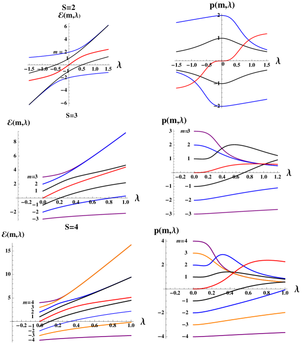
Figure 1: Reduced energies ${\cal E}(m,\lambda)$ and polarizations $p(m,\lambda)$ versus $\lambda$ for $S=2,3$ and 4. Since ${\cal E}(m,\lambda=0)=p(m,\lambda)=m$, intersection of the curves with the vertical axis $\lambda=0$ indicate their $m$ labeling. The $S=2$ curves exibit the symmetry relations ${\cal E}(m,\lambda)=-{\cal E}(-m,-\lambda)$ and $p(m,\lambda)=-p(-m,-\lambda)$, derived in the text. For $m>0$ there is a clear evidence for the degeneracies expected when $\lambda\gg 1$.

We present for $S=2,3$ and 4, explicit calcutations of the eigenenergies ${\cal E}(m,\lambda)$ and the polarization of the eigenstates, which, for symmetry reason, is along the ${\mathbf{B}}$ direction $p(m,\lambda)=\langle\hat{\psi}(m,\lambda)|S_{z}|\hat{\psi}(m,\lambda)\rangle$. (In this section, for the sake of simplicity we use a unit system where $\hbar=1$). We construct the matrix associated with ${\cal H}(S,\lambda)$within the angular momentum basis:$|S\,m\rangle$. It is convenient to rewrite the Hamiltonian in terms of the operators $S_{z},S^{+}=S_{x}+iS_{y}$ and $S^{-}=S_{x}-iS_{y}$

$${\cal H}(S,\lambda) = S_{z}+\lambda S_{x}^{2}\;,$$

$$\equiv S_{z}-\frac{\lambda}{2}S_{z}^{2}+\frac{\lambda}{4}((S^{+})^{2}+(S^{-})^{2})+\frac{\lambda}{2}S(S+1)\,.$$

Using textbook formulae, for the matrix elements of $(S^{\pm})^{2}$ in the $|S\,m\rangle$ basis it is easy to write ${\cal H}(S,\lambda)$ in matrix form. Using the invariance under the symmetry ${\cal T}_{3}$ introduced in subsection II.A, ${\cal H}(S,\lambda)$ can be written as a direct sum of two matrices acting respectively upon the states $|Sm\rangle$ with even and odd values of $S-m$, ${\cal H}(S,\lambda)={\cal H}_{even}(S,\lambda)\oplus{\cal H}_{odd}(S,\lambda),$ one of order $S$ and the other of order $(S+1)$ depending on the parity of S. For $S=1$ and 2 one finds easily:

$${\cal H}_{odd}(1,\lambda) = \left(\begin{array}[]{cc}\lambda/2+1&\lambda/2\\ \lambda/2&\lambda/2-1\end{array}\right),$$ (22)

$${\cal H}_{even}(2,\lambda) = \left(\begin{array}[]{ccc}\lambda+2&\sqrt{3/2}\;\lambda&0\\ \sqrt{3/2}\;\lambda&3\lambda&\sqrt{3/2}\;\lambda\\ 0&\sqrt{3/2}\;\lambda&\lambda-2\end{array}\right),$$ (26)

$${\cal H}_{odd}(2,\lambda) = \left(\begin{array}[]{cc}5\lambda/2+1&3\lambda/2\\ 3\lambda/2&5\lambda/2-1\end{array}\right).$$ (29)

The Hamiltonians ${\cal H}_{even}(3,\lambda)$ and ${\cal H}_{odd}(3,\lambda)$ as well as ${\cal H}_{even}(4,\lambda)$ and ${\cal H}_{odd}(4,\lambda)$ are given in Appendix B.

The eigenvalues are obtained in a standard way by solving the two polynomial equations:

$$\det(x\;\mathbf{l}-{\cal H}_{even}(2,\lambda)) \equiv x^{3}-5x^{2}\lambda+4x\lambda^{2}-4x+12\lambda$$

$$= 0,$$

$$\det(x\;\mathbf{l}-{\cal H}_{odd}(2,\lambda)) \equiv x^{2}-5x\lambda+4\lambda^{2}-1=0.$$ (30)

The eigenvalue equations for $S=3$ and $S=4$ can be found in the appendix. Mathematica codes yield explicit expressions for the eigenenergies ${\cal E}(m,\lambda)$. Although the formulae are rather complex, they lead to very accurate numerical results for all the values of $\lambda$ of interest. The accuracy is better than $10^{-12}$. This result has been checked using numerical Mathematica codes, obtained directly from the matrix expression. To calculate the polarization $p(m,\lambda)$ we have used the fact that it is given by the derivative of the eigenenergy with respect to $\gamma_{S}B$ (Hellmann-Feynman theorem). Writing the eigenvalue of $\hat{H}(B,E)$ as: ${\mathrm{E}}(m,B,E)=\gamma_{S}B\,{\cal E}(m,\lambda)$, with $\lambda=\frac{\hbar\gamma_{Q}E^{2}}{\gamma_{S}B}$, one gets immediately:

$$p(m,\lambda)=\frac{\partial\,{\mathrm{E}}(m,B,E)}{\hbar\gamma_{S}\,\partial\,B}={\cal E}(m,\lambda)-\lambda\frac{\partial{\cal E}(m,\lambda)}{\partial\,\lambda}.$$ (31)

The results are given in Fig.1 for both the energies and the polarizations. The eigenenergies ${\cal E}(m,\lambda)$ can be labelled unambiguously since for small values of $\lambda$ the eigenvalues are equal to $m$, up to corrections of the order of $\lambda^{2}$. In Fig.1 there is evidence for near-degeneracies of opposite-parity level pairs: ${\cal E}(m,\lambda)$ is approaching ${\cal E}(m-1,\lambda)$ when $\lambda\gg 1$ for $m=S-q$, where $q$ is an even integer such that $0\leq q<S$. This was expected since in this limit ${\cal H}(\lambda)$ is dominated by the term $\propto S_{x}^{2}$. The convergence is much slower for $m<0$ since the positive term $\lambda\,S_{x}^{2}$ term has then to fight against a negative Zeeman effect. There are $S$ degenerate doublets with ${\cal E}(m,\lambda)/\lambda\simeq m^{2}$, as expected in the limit $\lambda\gg 1$. In addition, by looking at the even-odd (or odd-even) pairs, one sees clearly that the pair ${\cal E}(S,\lambda),{\cal E}(S-1,\lambda)$ converges, without crossing, to the degenerate doublet ${\cal E}(S,\lambda)\simeq{\cal E}(S-1,\lambda)\simeq\lambda S^{2}.$ The next lower pair ends as the degenerate doublet having the energy $\simeq\lambda\,(S-1)^{2}$ and so on until one reaches the isolated level $m=-S$, which has no possibility other than converging towards the non-degenerate level with energy $\lambda\times 0$. While this behaviour is clearly exhibited in the simple case $S=2$, only its two first steps are clearly apparent for $S=3$ and 4 , but we have verified that the above picture is valid for all values of $m$ by computing the ratios ${\cal E}(m,\lambda)/\lambda$ when $\lambda\gg 1$.

A striking feature of the case $S=2$ in Fig.1 is the symmetry of the plotted curves under the transformation $m\rightarrow-m\,,\,\lambda\rightarrow-\lambda$, involving both the eigenenergies and the polarizations: ${\cal E}(m,\lambda)\rightarrow-{\cal E}(-m,-\lambda)$, $p(m,\lambda)\rightarrow-p(-m,-\lambda).$ To prove these symmetry properties in the general case, it is convenient to perform upon the spin system a rotation of angle $\pi$ around the $x$ axis, $R(\hat{x},\pi)$. By introducing the spin unitary operator $U(R(\hat{x},\pi))=\exp(-i\,S_{x}\,\pi),$ associated with the rotation $R(\hat{x},\pi)$, one can write the transformation law for the Hamiltonian ${\cal H}(\lambda)$:

$$U(R(\hat{x},\pi)){\cal H}(\lambda)U^{-1}(R(\hat{x},\pi))=-S_{z}+\lambda S_{x}^{2}=-{\cal H}(-\lambda).$$

Applying $U(R(\hat{x},\pi))$ to both sides of the eigenvalue equation ${\cal H}(\lambda)\hat{\psi}(m,\lambda)={\cal E}(m,\lambda)\hat{\psi}(m,\lambda)$, one can write:

$$U(R(\hat{x},\pi)){\cal H}(\lambda)\hat{\psi}(m,\lambda) = -{\cal H}(-\lambda)U(R(\hat{x},\pi))\hat{\psi}(m,\lambda)$$ (32)

$$={\cal E}(m,\lambda)U(R(\hat{x},\pi)\hat{\psi}(m,\lambda).$$

The state $U(R(\hat{x},\pi)\hat{\psi}(m,\lambda)$ is an eigenstate of ${\cal H}(-\lambda)$ with the eigenenergy $-{\cal E}(m,\lambda)$. It coincides, up to a phase factor, with the eigenstate $\hat{\psi}(-m,-\lambda)$, since the effect of the rotation $R(\hat{x},\pi)$ is to flip the spin component along the $z$ axis. This completes the proof that:

$${\cal E}(m,\lambda)=-{\cal E}(-m,-\lambda).$$

with the similar relation for $p(m,\lambda)$ as a consequence of Eq. (31).

In addition, the quantum-averaged polarizations $p(m,\lambda)$ satisfy the sum rule

$$\sum_{m}p(m,\lambda)=0,$$ (33)

valid for any value of S and $\lambda$. It is readily derived using the fact that $p(m,\lambda)$ can be evaluated as the partial derivative of the energy with respect to $\gamma_{S}B$ (Eq. (31)) and noting the general structure of the polynomial equation whose solutions provide the eigenenergies.

To end this section we would like to say a few words concerning the state $m=0$ which is of particular interest for integer spins $S\geq 2$. The fact that a second-order Stark effect can induce a polarization in an initially unpolarized state was somewhat unexpected. To gain greater insight we have performed a perturbation computation in powers of $\lambda$. Although one has to go to third order to find a non-zero effect the final result is given by the rather elegant formula:

$$p(0,\lambda)=\frac{1}{8}{\lambda}^{3}S(S+2)\left(S^{2}-1\right)\left(1+{\cal O}(\lambda^{2})\right).$$ (34)

It gives a rather accurate result for $S=2$ if $|\lambda|\leq 0.4$ but the domain of validity gets smaller for S=3: $|\lambda|\leq 0.12$. Finally we would like to point out the smooth behaviour of $p(0,\lambda$) for $S=2$ in the vicinity of $\lambda\simeq 1$ and the remarkably simple exact values taken by the reduced energy and the polarization at $\lambda=1$, namely ${\cal E}(0,1)=2$ and $p(0,1)=1$. At the time of writing, it is unclear whether this is a mere numerical accident or an indication of something more profound.

IV Berry’s phase for adiabatic cycles generated by $H({\mathbf{B}}(t),{\mathbf{E}}(t))$ acting on arbitrary spins

We start this section by a mini-review introducing the basic physical and mathematical features of Berry’s phase concept. In particular we derive the general formula giving the Berry’ phase in terms of the instantaneous eigenfunctions of the time-dependent Hamiltonian generating the adiabatic quantum cycles. Introducing in this formula, the results of the previous section and relying upon Group Theory arguments, we perform an explicit construction of Berry’s phase relative to $H({\mathbf{B}}(t),{\mathbf{E}}(t))$, valid for arbitrary spins. The final result is expressed as a loop integral in the ${\mathbf{C}}P^{2}$ space, using as coordinates the Euler angles and the parameter $\lambda$. We show that for the case $S=2$ a circular loop drawn upon a spherical subspace of ${\mathbf{C}}P^{2}$ lead to a loop integral very different from that of the case $S=1$ which involves a magnetic monopole Bohm-Aharonov phase.

IV.1 The Berry’s phase as a physical observable and topological concept: a mini-review

In this introductory subsection, we are going to follow, in several places, a presentation due to the late Leonard Schiff, in tribute of its memory. He gave in few pages of its venerable textbook [26] a correct and precise treatment of the adiabatic approximation, involving a non-integrable phase. To study the adiabatic quantum cycles generated by the Schrödinger equation

$$i\,\hbar\frac{\partial}{\partial t}\Phi(t)=H(t)\,\Phi(t)\hskip 14.22636pt\text{ where}\hskip 14.22636pt\,H(t)=H({\mathbf{B}}(t),{\mathbf{E}}(t)),$$

it is convenient to expand the solution $\Phi(t)$ in terms of the eigenstates of $H(t)$ :

$$\Phi(t)=\sum_{n}a_{n}(t)\exp\left(\frac{i}{\hbar}\,\chi(n,t)\right)\Psi(n,t),$$ (35)

$${\rm where}\;\;\;\chi(n,t)=\gamma(n,t)-\int_{0}^{t}dt_{1}{\mathrm{E}}(n,B(t_{1}),E(t_{1})).$$ (36)

The first term $\gamma(n,t)$ in (36) is a phase that vanishes for $t=0$, but is otherwise arbitrary. Its value will be determined by the reasoning leading to the adiabatic approximation. The second term,

$$\Phi_{D}(n)=-\frac{1}{\hbar}\int_{0}^{t}dt_{1}{\mathrm{E}}(n,B(t_{1}),E(t_{1})),$$ (37)

known as the “dynamical phase”, produces a contribution which cancels $H(t)\Phi(t)$ in the wave equation. We shall take as the initial condition : $\Phi(0)=\Psi(m,0)$ or, in other words, $a_{n}(0)=\delta_{n,m}$. In this case we can replace the exact Schrödinger equation by the system of differential equations involving the expansion coefficients $a_{n}(t)$:

$$i\,\hbar\,\dot{a}_{n}(t)=a_{n}(t)\,(\dot{\gamma}(n,t)-\langle\Psi(n,t)|i\,\hbar\frac{\partial}{\partial t}\Psi(n,t)\rangle)-$$

$$\sum_{k\neq n}a_{k}(t)\exp{i(\chi(k,t)-\chi(n,t))}\langle\Psi(n,t)|i\,\hbar\frac{\partial}{\partial t}\Psi(k,t)\rangle.$$ (38)

Since the adiabatic condition requires that $a_{n}(t)\approx 1$ whatever $t$, a necessary condition to ensure its validity is to cancel the coefficient of $a_{n}(t)$ in the r.h.s of equation (38). This is achieved if we make the following choice for the “gauge ” $\gamma(n,t)$:

$$\gamma(n,t)=\int_{0}^{t}dt_{1}\langle\Psi(n,t_{1})|\,i\,\hbar\frac{\partial}{\partial t}\Psi(n,t_{1})\rangle.$$ (39)

Later on, we shall see that this non integrable gauge is a basic ingredient in the mathematical expression of Berry’s phase in terms of the instantaneous wave functions $\Psi(m,t)$. The next step to validate the adiabatic approximation is to find appropriate conditions allowing the sum ${\sum_{n\neq m}|a_{n}(t)|}^{2}$ to remain below a predefined level for $t>0$. This task will be performed in details in Sec. V but for the moment, let us assume that it is achieved. Within the adiabatic approximation, the solution of the Schrödinger equation $i\,\hbar\frac{\partial}{\partial t}\Phi(t)=H(t)\,\Phi(t)$, with the initial condition $\Phi(0)=\Psi(m,0)$, is then given by:

$$\Phi_{ADB}(m,t)=$$

$$\exp\frac{i}{\hbar}\left(\gamma(m,t)-\int_{0}^{t}dt_{1}{\mathrm{E}}(m,B(t_{1}),E(t_{1}))\right)\Psi(m,t).$$ (40)

We can now calculate the phase shift of the wave function $\Phi_{ADB}(m,t)$ at the end of the adiabatic cycle:

$$\arg\left(\frac{\Phi_{ADB}(m,T)}{\Phi_{ADB}(m,0)}\right) = \arg\left(\frac{\Psi(m,T)}{\Psi(m,0)}\right)+$$ (41)

$$\frac{1}{\hbar}\left(\gamma(m,T)-\int_{0}^{T}dt\,{\mathrm{E}}(m,B(t),E(t))\right),$$

$$=-\frac{1}{\hbar}\int_{0}^{T}dt\,{\mathrm{E}}(m,B(t),E(t))+\beta(m),$$

where we have made Berry’s phase $\beta(m)$ stand out on the r.h.s of the above equation. Using the equation (39), one gets immediately the basic formula giving $\beta(m)$ in terms of the instantaneous wave functions $\Psi(m,t)$:

$$\beta(m) = \int_{0}^{T}dt\langle\Psi(m,t)|\,i\,\frac{\partial}{\partial t}\Psi(m,t)\rangle+\phi(m),$$

$$\phi(m) = \arg\left(\Psi(m,T)/\Psi(m,0)\right).$$ (42)

It is crucial to note that the “dynamical phase ” $\phi_{D}(m)$ and $\beta(m)$ obey different scaling laws under the transformation, $B\rightarrow\xi B$, involving an arbitrary real parameter $\xi$, while keeping invariant the Euler angles and the dimensionless parameter $\lambda$. If one remembers that ${\mathrm{E}}(m,B(t),E(t))=\gamma_{S}B\,{\cal E}(m,\lambda(t))$, one sees immediately that $\phi_{D}(m)$ is multiplied by $\xi$, while $\beta(m)$, being geometric, is unchanged. In principle, this scaling difference could be used to separate the two phases. However, a more practical way to isolate Berry’s phase consists in measuring the phase for a given adiabatic cyclic evolution and that associated with the “image” circuit obtained by performing on the Hamiltonian parameters the transformations: $\alpha(t)\rightarrow-\alpha(t)\,,\,\varphi(t)\rightarrow-\varphi(t)$, while keeping the other two unchanged. The two competing phases are transformed as $\phi_{D}(m)\rightarrow\phi_{D}(m)\,,\,\beta(m)\rightarrow-\beta(m)$, so that the dynamical phase can be eliminated by subtraction.

To end this mini-review, we would like to give, within the present context, a simplified description of the topological interpretation of the Berry’s Phase, due to Simon [2]. We have just shown that $\Phi_{ADB}(m,t)$ is a physical state obeying the Schrödinger equation within the adiabatic approximation. For our purpose, it is convenient to introduce the $mathematical$ vector state $\Phi_{\parallel}(m,t)=\exp\left(-i\phi_{D}(m,t))\right)\Phi_{ADB}(m,t)$ and to calculate the differential form $\langle\Phi_{\parallel}|d\Phi_{\parallel}\rangle=\langle\Phi_{\parallel}(m,t)|\frac{\partial}{\partial t}\Phi_{\parallel}(m,t)\rangle\,dt$ taken along the adiabatic loop:

$$\langle\Phi_{\parallel}|d\Phi_{\parallel}\rangle = \langle\Phi_{ADB}|-i\frac{\partial}{\partial t}\phi_{D}(m,t)\Phi_{ADB}\rangle\,dt+$$

$$\langle\Phi_{ADB}|\frac{1}{i\hbar}H(t)\Phi_{ADB}\rangle\,dt=0.$$

The evolution of the state vector $\Phi_{\parallel}$ along the closed loop is then said to satisfy the “parallel transport” condition $\langle\Phi_{\parallel}|d\Phi_{\parallel}\rangle=0$. If the state $\Phi_{\parallel}(t)$ is injected into the general formula for the Berry’s phase, one immediately finds that

$$\beta(m)=\arg(\frac{\Phi_{\parallel}(m,T)}{\Phi_{\parallel}(m,0)}),$$ (43)

in the case of parallel transport.

Let us now give a rather elementary introduction to the mathematical concepts behind the above notion of “parallel transport” applied to the evolution of quantum states. This arises rather naturally from a linear fiber bundle interpretation of Quantum Mechanics. The linear fiber bundle associated with the quantum state space is constructed from the “base space” $E(\rho)$ of the “pure ” state density matrix $\rho=|\Psi\rangle\langle\Psi|$. Assuming for simplicity that the states $\Psi$ have unit norms, one finds that $\rho$ satisfies the simple nonlinear relation $\rho^{2}=\rho$. This implies clearly that $E(\rho)$ has a non-trivial topology. The “fiber” is the one-dimensional space associated with a definite $\rho$. The vector states of the fiber are given by $\Phi=\exp(i\phi)\Psi$, where $\phi$ is an arbitrary phase and $\Psi$ a representative state of the fiber. The infinitesimal variation $d\Phi$ during the quantum cycle is said to be “vertical” if it takes place along the fiber: $d\Phi_{V}=d\tau\,\Phi_{V}$, where $d\tau$ is an infinitesimal $c$-number. Conversely, it is called “horizontal” or “parallel” if $\langle\Phi_{\parallel}|d\Phi_{\parallel}\rangle=0$. The fact that the Berry’s phase can be viewed as a displacement respective to the fiber, associated with $\rho(0)=\rho(T)$ - in our case a phase shift resulting from a parallel transport along a closed loop drawn upon the base space $E(\rho)$ - emphasizes its topological character.

IV.2 The Berry’s phase as a loop integral in the Hamiltonian $H({\mathbf{B}}(t),{\mathbf{E}}(t))$ parameter space

Our starting point is the formula (42) giving Berry’s phase for quantum adiabatic cycles associated with the instaneous wave function $\Psi(m,t)$.

The fundamental property of $\beta(m)$ is its invariance under the gauge transformation $\Psi(m,t)\rightarrow\exp\left(\frac{i}{\hbar}f(t)\right)\,\Psi(m,t)$, where $f(t)$ is an arbitrary real function. The density matrix of an isolated quantum system has clearly the same gauge invariance property. The adiabatic approximation allows us to make a mapping of the Hamitonian parameter space onto the density matrix space. As a consequence, $\beta(m)$ could also be viewed as a line integral along a closed path drawn in the density matrix space.

A group theoretical derivation

To evaluate the expression (42), it is convenient to write $\beta(m)$ in terms of $\hat{\psi}(m,\lambda)$:

$$\beta(m)-\phi(m)=\int_{0}^{T}dt\langle\hat{\psi}(m,\lambda(t)|i\,\frac{\partial}{\partial t}\hat{\psi}(m,\lambda(t))\rangle+$$

$$\int_{0}^{T}dt\,\langle\hat{\psi}(m,\lambda(t))|U^{-1}(R(t))i\,\frac{\partial}{\partial t}\,\left(U(R(t))\right)|\hat{\psi}(m,\lambda(t)\rangle.$$ (44)

Since $|\hat{\psi}(m,\lambda(t)\rangle$ is a real vector in the $|S,m\rangle$ basis, the first term of the integral can be written as:

$$\frac{i}{2}\frac{\partial}{\partial t}\{\Sigma_{{}_{\mu=-S}}^{{}^{\mu=S}}\;[\langle S,\mu|\hat{\psi}(m,\lambda(t)\rangle]^{2}\}\;.$$

If the cyclic condition $\lambda(T)=\lambda(0)$ is satisfied, the line integral of this term is zero. If now one uses the explicit form of $U(R(t))$ in terms of the spin operator ${\mathbf{S}}$ (Eq. (15), it is easily seen that the second term of Eq.(44) is a linear combination of time derivatives of the Euler angles:

$$i\hbar U^{-1}(R(t))\frac{\partial}{\partial t}\,(U(R(t))=\dot{\alpha}\;D_{\alpha}+\dot{\theta}\;D_{\theta}+\dot{\varphi}\;D_{\varphi}\,.$$ (45)

Let us consider $D_{\alpha}$:

$$D_{\alpha}=\exp{(\frac{i}{\hbar}S_{z}\alpha(t))}\cdot\exp{(\frac{i}{\hbar}S_{y}\theta(t))}\cdot\exp{(\frac{i}{\hbar}S_{z}\varphi(t))}\times$$

$$\exp{(-\frac{i}{\hbar}S_{z}\varphi(t))}\cdot\exp{(-\frac{i}{\hbar}S_{y}\theta(t))}\cdot S_{z}\cdot\exp{(-\frac{i}{\hbar}S_{z}\alpha(t))}.$$

Since $S_{z}$ commutes with the exponential $\exp{(-\frac{i}{\hbar}S_{z}\alpha(t))}$, $D_{\alpha}$ reduces to:

$$D_{\alpha}=U^{-1}(R(t))U(R(t))S_{z}=S_{z}.$$ (46)

For the two remaining terms such as $D_{\varphi}$ the calculation is not so simple. Using the fact that $S_{z}$ commutes with $\exp{(-\frac{i}{\hbar}S_{z}\varphi(t))}$, one can write

$$D_{\varphi} = \exp{(\frac{i}{\hbar}S_{z}\alpha(t))}\cdot\exp{(\frac{i}{\hbar}S_{y}\theta(t))}\times$$

$$S_{z}\cdot\exp{(-\frac{i}{\hbar}S_{y}\theta(t))}\cdot\exp{(-\frac{i}{\hbar}S_{z}\alpha(t))}.$$

Using equation(12), one can derive the commutation relation:

$$S_{z}\cdot\exp{(-\frac{i}{\hbar}S_{y}\theta(t))}=\exp{(-\frac{i}{\hbar}S_{y}\theta(t))}\cdot(S_{z}\cos{\theta}-S_{x}\sin{\theta})\,.$$

After repeating a similar operation to push $\exp{(-\frac{i}{\hbar}S_{z}\alpha(t))}$ to the left of $(S_{z}\cos{\theta}-S_{x}\sin{\theta})$, one arrives finally at the following expression:

$$D_{\varphi}=S_{z}\cos{\theta}+\sin{\theta}(-S_{x}\cos{\alpha}+S_{y}\sin{\alpha})\,.$$ (47)

In a similar way one obtains

$$D_{\theta}=S_{y}\cos{\alpha}+S_{x}\sin{\alpha},$$ (48)

but this term will not lead to any contribution to $\beta$ because of the boundary condition: $\theta(T)=\theta(0)$. Since the quantum average of ${\mathbf{S}}$ relative to the state $\hat{\psi}(m,\lambda)$ has a single component along $\hat{z}$, we end up with the compact expression:

$$\beta(m)-\phi(m)=\int_{0}^{T}p(m,\lambda(t))(\cos{\theta}\;\dot{\varphi}+\dot{\alpha})dt\,.$$ (49)

We now have to calculate the phase shift $\phi(m)=\arg\left\{\Psi(m,T)/\Psi(m,0)\right\}$ appearing in Eq (42). A preliminary step is to rewrite the unitary transformation $U(R(t))$ under a modified form:

$$U(R(t)) = V(t)\,\exp\left(-\frac{i}{\hbar}\,S_{z}(\varphi(t)+\alpha(t))\right),$$

$$V(t) = \exp\left(-\frac{i}{\hbar}\ S_{z}\,\varphi(t)\right)\times$$ (50)

$$\,\exp\left(-\frac{i}{\hbar}\,S_{y}\,\theta(t)\right)\,\exp\left(\frac{i}{\hbar}\,S_{z}\,\varphi(t)\right).$$

The transformation law given by equation (12) can be extended to any tensor operator $S_{i}\,S_{j}\,S_{k}\,...$ and consequently to any analytical function of $S_{y}$. Using the extended law, one can write $V(t)$ in the compact form:

$$V(t)=\exp\left(-\frac{i}{\hbar}\theta(t)(\cos\varphi(t)\,S_{y}+\sin\varphi(t)\,S_{x})\right).$$ (51)

Using the boundary conditions $\theta(T)=\theta(0),\lambda(T)=\lambda(0),\alpha(T)=\alpha(0)+n_{\alpha}\pi$ and $\varphi(T)=\varphi(0)+2n_{\varphi}\pi,$ one obtains the relation: $V(T)=V(0)$. Introducing for convenience the notation $U(\hat{z},u)=\exp\left(-\frac{i}{\hbar}\,S_{z}\,u\right)$ it is then possible to rearrange $\Psi(m,T)$ as follows:

$$\Psi(m,T) = V(0)\,U(\hat{z},\varphi(T)+\alpha(T))\hat{\psi}(m,\lambda(0)),$$ (52)

$$=V(0)\,U(\hat{z},\varphi(0)+\alpha(0))\,U(\hat{z},\Delta\varphi+\Delta\alpha)\hat{\psi}(m,\lambda(0)),$$

$$\text{with}\;\;\;\Delta\varphi+\Delta\alpha=\varphi(T)+\alpha(T)-\varphi(0)-\alpha(0),$$

$$\hskip 19.91692pt=(2n_{\varphi}+n_{\alpha})\pi.$$

The next step is to prove that $\hat{\psi}(m,\lambda(0))$ is an eigenstate of $U(\hat{z},\Delta\varphi+\Delta\alpha)$ using its expansion in terms of the angular momentum state vectors $|S,q\rangle$, eigenstates of $S_{z}$ of eigenvalue $\hbar q$:

$$\hat{\psi}(m,\lambda(0))=\sum_{|m-2n|\leq S}C_{m,n}(\lambda(0))|S,m-2n\rangle.$$ (53)

Using equations (52), one sees immediately that, as a consequence of the quantum cycle boundary conditions, each state $|S,m-2n\rangle$ appearing in the above sum is an eigenstate of $U(\hat{z},\Delta\varphi+\Delta\alpha)$ with the eigenvalue $\exp\left(-i\,m\,\pi(2\,n_{\varphi}+n_{\alpha})\right)$. This leads to the basic relation connecting $\Psi(m,T)$ and $\Psi(m,0)$:

$$\Psi(m,T) = \exp\left(-i\,m\,\pi(2\,n_{\varphi}+n_{\alpha})\right)\times$$ (54)

$$V(0)\,U(\hat{z},\varphi(0)+\alpha(0))\hat{\psi}(m,\lambda(0))$$

$$= \exp\left(-i\,m\,(\Delta\varphi+\Delta\alpha)\right)\,\Psi(m,0).$$

One immediately obtains the phase shift $\phi(m)$ appearing on the r.h.s of equation (42):

$$\phi(m) = \arg\left\{\Psi(m,T)/\Psi(m,0)\right\}$$ (55)

$$= -m(\varphi(T)-\varphi(0)+\alpha(T)-\alpha(0))$$

$$= -m\int_{0}^{T}(\dot{\varphi}(t)+\dot{\alpha}(t))\;dt\;.$$

By combining the equations (49) and (55), we arrive at the expression of Berry’s phase for an arbitrary quantum adiabatic cycle generated by the Hamiltonian $H({\mathbf{B}}(t),{\mathbf{E}}(t))$ of equation (1) with ${\mathbf{E}}(t)\cdot{\mathbf{B}}(t)=0$

$$\beta(m) = -\int_{0}^{T}[m-p(m,\lambda(t))\cos{\theta(t)}]\,\dot{\varphi}(t)\;dt$$ (56)

$$-\int_{0}^{T}[m-p(m,\lambda(t))]\;\dot{\alpha}(t)\;dt\,.$$

The Berry’s phase as a loop integral of an Abelian Gauge Field

The Berry’s phase $\beta(m)$ given by equation (56) can be written as a loop integral around a closed curve ${\cal C}$ drawn in the parameter space ${\mathbf{C}}P^{2}$, using $\lambda,\theta,\varphi,\alpha$ as coordinates:

$$\beta(m)=-\oint_{{\cal C}}\left((m-p(m,\lambda)\cos\theta)d\varphi+(m-p(m,\lambda))d\alpha\right).$$ (57)

The above formula suggests that $\beta(m)$ could be written as a loop line integral of an Abelian gauge field $A_{i}(x_{j})$, defined in the parameter space. The non-vanishing components of the gauge field candidate, $A_{\varphi}$ and $A_{\alpha}$, are then given by:

$$A_{\varphi}=-m+p(m,\lambda)\cos\theta,\;\;\;\;\;\;A_{\alpha}=-m+p(m,\lambda).$$ (58)

Thus the Berry’s phase looks like the Bohm-Aharonov phase [29], for the Abelian gauge field $(A_{\varphi},A_{\alpha)})$:

$$\beta(m)=\oint_{{\cal C}}(A_{\varphi}\,d\varphi+A_{\alpha}d\alpha).$$ (59)

What remains to be proved is that the above expression is indeed invariant under the gauge transformation of the Abelian field:

$$A_{\varphi}\rightarrow A_{\varphi}+\frac{\partial}{\partial\varphi}g(\varphi,\theta,\alpha,\lambda),\;\;\;A_{\alpha}\rightarrow A_{\alpha}+\frac{\partial}{\partial\alpha}g(\varphi,\theta,\alpha,\lambda).$$ (60)

The crucial point is that $g(\varphi,\theta,\alpha,\lambda)$ must be a single-valued function of ${\mathbf{B}}$ and ${\mathbf{E}}\otimes{\mathbf{E}}$, like the gauge field itself. This implies that $g(\varphi,\theta,\alpha,\lambda)$ must be a periodic function of $\varphi$ and $\alpha$, with periods respectively of $2\pi$ and $\pi$. Remembering the boundary conditions (II.2) for the quantum cycle ${\cal C}$ , one finds immediately that the gauge contributions to $\beta(m)$, $g(\varphi(0)+2n_{\varphi}\,\pi,\theta(0),\alpha(0)+n_{\alpha}\,\pi,\lambda(0))-g(\varphi(0),\theta(0),\alpha(0),\lambda(0))$, do indeed vanish. This completes the identification of $\beta(m)$ as a Bohm-Aharonov phase.

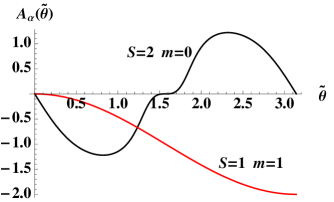
Figure 2: Representation of the gauge field component $A_{\alpha}(\tilde{\theta})$ versus the associated $\tilde{\theta}$ parameter of the non-linear Hamiltonian in the two cases $S=1$ (red curve) and $S=2$ (black curve). The difference between the two graphs illustrates the fact that for $S>1$ there is no longer a one to one correspondence between the Hamiltonian parameter space and the density matrix space upon which is drawn the quantum cycle. The non-linear spin Hamiltonian generates a new geometry revealed only by spins larger than one.

Berry’s phase geometry generated by non-linear spin Hamiltonians for $S>1$

For the sake of simplicity, in the next sections we shall concentrate on Berry’s cycles where $\lambda$ and $\alpha$ are the only time-varying parameters. The question then arises as to whether we shall not lose in this way most of the new features introduced with the non-linearity of $H(t)$. In order to make clear the cause for our concern, let us perform the change of variables upon the two left-over parameters which map the associated 2D manifold onto a 2D sphere: $\lambda=-2\cot(\tilde{\theta})$ with $0<\tilde{\theta}<\pi$ and $\tilde{\varphi}=2\,\alpha$. In ref. [24] we have given an explicit form of the ${\mathbf{C}}P^{2}$ metric obtained with this kind of coordinates. For the sub-manifold associated with $\tilde{\dot{\varphi}}=\tilde{\dot{\theta}}=0$ it turns out that this metric, $ds^{2}=\frac{1}{4}\left(d\tilde{\varphi}^{2}\sin^{2}\,\theta+d\tilde{\theta}^{2}\right)$ is identical to the one associated with a 2D sphere having a radius 1/2 (this factor results from the choice: $\tilde{\varphi}=2\,\alpha$.)

To answer the question, we can now consider the component of the gauge field $A_{\alpha}$ for two different cases. For $S=1,m=1$, the gauge field is given by the same expression as the gauge field associated with a linear Hamiltonian $A_{\alpha}(\tilde{\theta})=\cos\tilde{\theta}-1$. However, the situation is totally different for the case $S=2,m=0$, where $A_{\alpha}(\tilde{\theta})$ exhibits the peculiar shape shown in Fig.2. This implies that the geometry involved in Berry’s phase for the sub-manifold differs from its usual interpretation in terms of the solid angle defined by a closed loop drawn upon a 2D sphere. The origin of this phenomenon lies in the fact that the density matrix space for $S=2$ is not ${\mathbf{C}}P^{2}$ but rather ${\mathbf{C}}P^{4}$. Unlike the case $S=1$, there is no longer a one to one correspondence between the parameter space and the density matrix space. It is thus not surprising that the geometry involved in Berry’s phase for a non-linear Hamiltonian should differ from the linear case, even for the simple cycles involving only the variations of the two parameters $\lambda$ and $\alpha$.

V Non-adiabatic corrections in Berry’s cycles using the rotating frame Hamiltonian

For quantum cycles of finite duration $T$, the time derivatives of the Hamiltonian parameters cannot take arbitrary small values. For instance, in the experiments discussed in a separate paper [5], the quadratic spin coupling generated by an ac Stark effect induces an atomic instability when $\lambda\approx 1$. As a result, the measurement of Berry’s phases studied by interferometry experiments on alkali atoms will require a good control upon the non-adiabatic corrections arising from the time dependent external ${\mathbf{B}},{\mathbf{E}}$ fields.

We shall consider separately the effect coming from the periodic parameters $\alpha$ and $\varphi$ in subsections V.A and V.B, and the non-periodic one $\lambda$ in subsection V.C. Our method involves the time-dependent Schrödinger equation in the rotating frame. We shall use an adiabatic approximation within this frame, the slowly varying parameters being, then, the time derivatives of the periodic parameters $\dot{\alpha}$ and $\dot{\varphi}$.

We set $\Phi(t)=U(R(t))\widetilde{\Phi}(t)$, and we write the wave equation relative to $\widetilde{\Phi}(t)$ in the rotating frame:

$$\left(i\hbar\frac{d}{dt}-\hat{H}(B(t),E(t))\right)\widetilde{\Phi}(t)=$$

$$-U^{-1}(R(t))\,i\hbar\frac{d}{dt}\,U(R(t))\,\widetilde{\Phi}(t)=$$

$$-(D_{\alpha}\,\dot{\alpha}+D_{\varphi}\,\dot{\varphi}+D_{\theta}\,\dot{\theta})\,\widetilde{\Phi}(t)=\gamma_{S}\,{\mathbf{S}}\cdot\Delta{\mathbf{B}}(t)\,\widetilde{\Phi}(t).$$ (61)

The rotating frame Hamiltonian can be written as

$${\widetilde{H}}(t)=\hat{H}(B(t),E(t))+\gamma_{S}{\mathbf{S}}\cdot\Delta{\mathbf{B}}(t),$$ (62)

where $\Delta{\mathbf{B}}(t)$ is an additional effective magnetic field generated by the Coriolis effect. It can be decomposed into a longitudinal component ${\Delta{\mathbf{B}}}_{//}(t)$ and a transverse one ${\Delta{\mathbf{B}}}_{\perp}(t)$. Using the explicit expressions of $D_{\alpha}$ and $D_{\varphi}$ in subsection III.B and assuming here -for the sake of simplicity- that $\dot{\theta}=0$, one arrives at the following expressions for of the effective field:

$${\Delta{\mathbf{B}}}_{//} = -\gamma_{S}^{-1}\,(\cos\theta\;\dot{\varphi}+\dot{\alpha})\,\hat{z}$$

$${\Delta{\mathbf{B}}}_{\perp} = -\gamma_{S}^{-1}\,\sin\theta\;\dot{\varphi}\,(-\cos\alpha\,\hat{x}+\sin\alpha\,\hat{y})$$ (63)

$$= \gamma_{S}^{-1}\,\sin\theta\;\dot{\varphi}\,{\cal R}(\hat{z},-\alpha)\,\hat{x}.$$

The role of those two components are going to be examined separately.

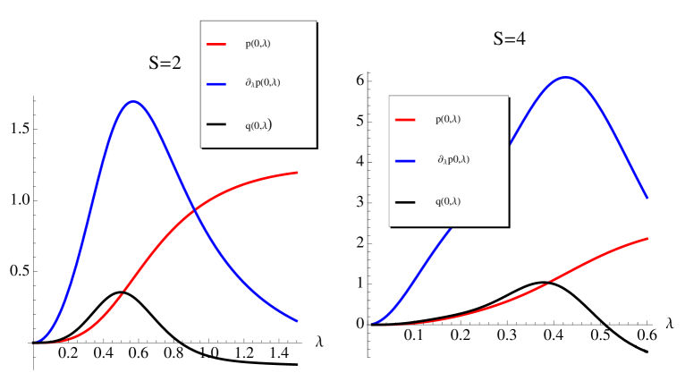
Figure 3: Comparison of Berry’s phase to its lowest-order non-adiabatic corrections, when $\alpha$ is the only time-dependent Euler angle, for a quantum cyle involving the spin configurations $S=2$, or 4 and $m=0$. The Berry’s phase is given by $\beta(0)=\int_{0}^{T}dt\,p(0,\lambda(t))\dot{\alpha}(t)$. Using the results of subsection V.A, one finds that the non-adiabatic correction is given by : $\Delta_{//}^{(2)}\beta(0)=\int_{0}^{T}dt\,q(0,\lambda(t))\dot{\alpha}(t)\,(\frac{\dot{\alpha}(t)}{\gamma_{S}\,B(t)})^{2}$. The explicit expression of $q(m,\lambda)$ in terms of the second- and third-order derivatives of ${\cal E}(m,\lambda)$ with respect to $\lambda$ can be found in Eq. (71). One sees clearly that, for $S=2$, if the parameter $\lambda$ is required to stay within the small interval $0.8\pm 0.2$, then $\Delta_{//}^{(2)}\beta(0)/\beta(0)$ will be $<10^{-3}$ provided $\dot{\alpha}(t)$ is kept smaller than one tenth of the Larmor angular frequency $\gamma_{S}\,B(t)$. Similarly, for $S=4$, there is a value of $\lambda$, for which $q(0,\lambda)$ cancels. The partial derivative $\frac{\partial}{\partial\lambda}p(0,\lambda)$ is governing the response of $\beta(0,\lambda)$, say, to a small variation of the $B$ field, are nearly at their maximum when $q(0,\lambda)$ is close to 0. Note also the fourfold increase of the sensitivity for $S=4$ compared to $S=2$.

V.1 The Berry’s phase and its non-adiabatic corrections involving the longitudinal effective magnetic field $(B(t)+\Delta B_{//}(t))\,\hat{z}$

We consider, first, the part of the Hamiltonian governing the evolution of $\widetilde{\Phi}(t)$ associated with ${\Delta{\mathbf{B}}}_{//}$, which is the sole present if $\dot{\varphi}=0$. This part can be written very simply in terms of $\hat{H}(B,E)$

$$\widetilde{H}_{//}(t)=\hat{H}(B(t)+\Delta B_{//}(t),E(t)).\;\;\\$$ (64)

To proceed it is convenient to introduce the dimensionless parameter $\eta$ :

$$\eta=-\frac{\Delta B_{//}}{B}=\frac{\cos{\theta}\,\dot{\varphi}+\dot{\alpha}}{\gamma_{S}\,B}.$$ (65)

Using $\widetilde{B}=(1-\eta)B$, the eigenvalues of $\widetilde{H}_{//}(t)$ are simply

$${\mathrm{E}}(m,B+\Delta B_{//},E) = \gamma_{S}\widetilde{B}\hbar\,\mathcal{E}(m,\tilde{\lambda})$$ (66)

$$= \gamma_{S}\,B\hbar\,(1-\eta)\,\mathcal{E}(m,\frac{\lambda}{1-\eta})$$

Since the quantum cycles generated by $\widetilde{H}_{//}(t)$ are devoid of any topology, we can expect Berry’s phase relative to the laboratory frame to be buried inside the dynamical phase of $\widetilde{H}(t)$:

$$\tilde{\phi}_{D\,//}(\lambda,\eta,m)=-\int_{0}^{T}dt\,\gamma_{S}\,B(1-\eta)\mathcal{E}(m,\frac{\lambda}{1-\eta}).$$ (67)

Indeed, it is easily seen that Berry’s phase is given by the first-order contribution in the $\eta$-series expansion of the above integral :

$$\tilde{\phi}_{D\,//}^{(1)}(\lambda,\eta,m) = \int_{0}^{T}dt\,\eta\,\gamma_{S}\,B\left(\mathcal{E}(m,\lambda)-\lambda\frac{\partial{\mathcal{E}}(m,\lambda)}{\partial\,\lambda}\right),$$ (68)

$$= \int_{0}^{T}dt\;p(m,\lambda)\,(\cos{\theta}\,\dot{\varphi}+\dot{\alpha}),$$

$$= \,\beta(m)-\phi(m),$$

where we have used equation (31) of sec. III. The phase $\phi(m)$ is recovered by returning to the laboratory frame. The even-order contributions $\propto\eta^{2p}$ are eliminated by subtracting term by term those coming from image circuits associated to opposite signs of the $\eta$-parameter (i. e. $\varphi\rightarrow-\varphi$ and $\alpha\rightarrow-\alpha$).

We now show that it is possible to find a magic value of $\lambda=\lambda^{\star}(\eta)$ that leads to a cancellation of all the contributions of the dynamical phase $\propto\eta^{2p+1}$. More precisely let us define

$$\Delta\beta_{//} = \frac{1}{2}\left(\tilde{\phi}_{D\,//}(\lambda,\eta,m)-\tilde{\phi}_{D\,//}(\lambda,-\eta,m)\right)-\beta(m)+\phi(m)$$ (70)

$$= \int_{0}^{T}dt(\cos{\theta}\,\dot{\varphi}+\dot{\alpha})\,\Delta p(m,\lambda,\eta),$$

$$\text{where}\;\;\;\Delta p(m,\lambda,\eta)=$$

$$\frac{1}{2\eta}\left(\eta+1)\mathcal{E}(m,\frac{\lambda}{1+\eta})-(\eta\rightarrow-\eta)\right)-p(m,\lambda).$$

The above formula seems to suggest that the integrand in the expression giving $\Delta\beta_{//}(m)$ is singular when $\eta=\pm 1$. In fact it is easily seen that this is not the case. Indeed, the ratios $\mathcal{E}(m,\lambda)/\lambda$ converge towards the eigenvalues of $(S_{x}/\hbar)^{2}\,:\,0,1,4...S^{2}$ , as $\lambda\rightarrow\infty$. As a preliminary step, let us consider the lowest-order expansion of the r.h.s of $\Delta p(m,\lambda,\eta)$ with respect to $\eta$

$$\Delta\beta_{//}^{(2)}(m) = \int_{0}^{T}dt\,\left(\cos{\theta}\,\dot{\varphi}+\,\dot{\alpha}\right)q(m,\lambda)\,\eta^{2},$$

$$q(m,\lambda) = \frac{-1}{6}\left(\lambda^{3}\,{\cal E}^{{}^{\prime\prime\prime}}(m,\lambda)+3\,\lambda^{2}\,{\cal E}^{{}^{\prime\prime}}(m,\lambda)\right).$$ (71)

Fig.3 shows the variations of $q(m,\lambda)$ versus $\lambda$ in the cases $S=2$ and 4, for $m=0$. A quite remarkable effect, clearly visible on Fig.3, is the vanishing of $q(0,\lambda$) for a particular value of $\lambda$ , in the vicinity of the maximun of $\frac{\partial}{\partial\lambda}p(0,\lambda)$. This should allow for rather accurate determinations of $\beta(0)$, as explained in the caption of Fig.3.

In the case where $\alpha$ is the sole time-dependent parameter we have found, that a similar property holds in fact to all orders in $\eta$. More precisely, we have shown that there exists for a given value of $\eta$ a “magic” value $\lambda^{\star}(S,\eta)$ such that the non-adiabatic correction to $p(m,\lambda)$ cancels exactly.

$$\Delta p(0,\lambda^{\star}(S,\eta),\eta)=0.$$ (72)

The magic values can be accurately represented by the polynomial fits given below:

$$\lambda^{\star}(2,\eta) = 0.838213-0.0837823\eta^{2}-0.0431478\eta^{4}-$$

$$0.0231887\eta^{6}-0.0207986\eta^{8}$$

$$\lambda^{\star}(4,\eta) = 0.509982-0.0900927\eta^{2}-0.0349985\eta^{4}-$$ (73)

$$0.0436495\eta^{6}+0.0373634\eta^{8}$$

As it is apparent upon the above formulas, the “magic” values $\lambda^{\star}(S,\eta)$ are slowly varying functions of $\eta$ within the interval $0\leq\eta\leq 0.5$. We have verified that they both satisfy the equation (72) with a precision better than $3\times 10^{-7}$. In conlusion, the above results open the road to measurements of the Berry’s Phase $\beta(0)$ for $S=2$ and $S=4$, for quantum cycles where $\alpha$ is the sole varying Euler angle, under conditions where the non-adiabatic corrections can be kept below the one ppm level.

V.2 Non-adiabatic corrections induced by the effective transverse magnetic field ${\Delta{\mathbf{B}}}_{\perp}(t)$

This subsection is divided into two parts. In the first we calculate the corrections to the Berry’s phase of the laboratory frame that are odd under $\eta$-reversal. These arise from the modification of the dynamical phase induced by $\Delta{\mathbf{B}}_{\perp}(t)$. Then we turn to the small Berry’s phase in the rotating frame associated with the non-trivial topology of the quantum cycles. It arises from the time variation of the effective field $B(t)\,{\hat{z}}+\Delta{\mathbf{B}}(t)$ acting in the rotating frame. Let us stress again an important feature of the transverse contribution, $\gamma_{S}{\mathbf{S}}\cdot{\Delta{\mathbf{B}}}_{\perp}(t)$ to ${\widetilde{H}}(t)$. Being proportional to $\cos\alpha S_{x}-\sin\alpha S_{y}$, it mixes states of opposite $m$-parity which can be nearly degenerate, unless severe restrictions are imposed upon the domain of variation of $\lambda$. These constaints are directly read off from Fig.1. For $S=4,m=1,2$ and 3, only negative values of $\lambda$ are allowed, $-2\leq\lambda\leq 0$. For $S=2,m=0$ a larger interval can be used: $|\lambda|\leq 1$.

V.2.1 Correction to the dynamical phase

It is convenient to introduce the dimensionless parameters $\mu$ and $\widetilde{\mu}$ and the dimensionless operator ${\mathbf{\Sigma}}=\hbar^{-1}{\mathbf{S}}$:

$$\mu=-\frac{{\Delta B}_{\perp}}{B}=\frac{\sin\theta\,\dot{\varphi}}{\gamma_{S}\,B},\;\;\;\;\widetilde{\mu}=\frac{\mu}{1-\eta}.$$ (74)

We rewrite $\widetilde{H}(t)$ as follows:

$$\widetilde{H}(t)=\gamma_{S}\widetilde{B}\hbar\,({\cal H}(\tilde{\lambda})-\tilde{\mu}\,(-\cos\alpha\,\Sigma_{x}+\sin\alpha\,\Sigma_{y})).$$ (75)

To proceed, it is convenient to introduce the perturbation expansion of the eigenenergies of $\widetilde{H}(t)$:

$$\widetilde{E}(\tilde{\lambda},\tilde{\mu})=\gamma_{S}\widetilde{B}\hbar\,(\mathcal{E}(m,\tilde{\lambda})+\tilde{\mu}^{2}\,\mathcal{E}_{\perp}^{(2)}(m,\tilde{\lambda})+\mathcal{O}(\tilde{\mu}^{4})).$$ (76)

The second order energy shift caused by the $\widetilde{\mu}$-contribution to $\widetilde{H}(t)$ is given, to all orders in $\eta$, by:

$${\cal E}^{(2)}_{\perp}(m,\tilde{\lambda})=\sum_{|n-m|odd}\frac{|\langle\hat{\psi}(n,\tilde{\lambda})|\cos{\alpha}\,\Sigma_{x}-\sin{\alpha}\,\Sigma_{y}|\hat{\psi}(m,\tilde{\lambda})\rangle|^{2}}{\mathcal{E}(m,\tilde{\lambda})-\mathcal{E}(n,\tilde{\lambda})}.$$ (77)

The symmetry properties of $H(\lambda)$ (Sec.II) have two consequences i) only $|n-m|$-odd terms contribute to the sum and ii) the cross terms involving $\Sigma_{x}\Sigma_{y}$ cancel out. This means that there is no contribution proportional to $\sin{\alpha}\cos{\alpha}$. We are left with the terms prop to ${\cos{\alpha}}^{2}$ and ${\sin{\alpha}}^{2}$. We shall assume that the velocity $\dot{\alpha}$ is a slowly varying function of $t$ during the cycle, so that ${\cos{\alpha}}^{2}$ and ${\sin{\alpha}}^{2}$ can be replaced by their average values of 1/2.

At this point we have found convenient to solve numerically two auxiliary problems, namely the search of the eigenstates of the two Hamiltonians:

$${\cal H}_{i}(\lambda,\mu)={\cal H}(\lambda)-\mu\Sigma_{i}\;\;\;\text{for}\;\;\;i=x\;\;\;\text{and}\;\;\;i=y.$$

Let ${\mathcal{E}}_{x,y}(\lambda,\mu)$ be the individual eigenenergies of ${\mathcal{H}}_{x,y}$ which are even functions of $\mu$. To lowest-order in $\mu$, they take the form:

$$\mathcal{E}_{x,y}(\lambda,\mu)=\mathcal{E}(\lambda)+\mu^{2}\,\mathcal{E}^{(2)}_{x,y}(\lambda)+\mathcal{O}(\mu^{4}),$$ (78)

where ${\cal E}^{(2)}_{x,y}(\lambda)$ are obtained by an interpolation towards $\mu=0$. The overall second order energy shift of Eq.(77) can be expressed as:

$$\mathcal{E}^{(2)}_{\perp}(m,\tilde{\lambda})=\frac{1}{2}({\cal E}^{(2)}_{x}(\tilde{\lambda})+{\cal E}^{(2)}_{y}(\tilde{\lambda})).$$ (79)

We have now all we need to write the contribution to the dynamical phase associated with $\widetilde{H}(t)$ to 2nd-order in $\mu$ and all orders in $\eta$:

$$\phi^{(2)}_{D\perp} = -\int_{0}^{T}dt\,\gamma_{S}\,\widetilde{B}\,\tilde{\mu}^{2}\,\mathcal{E}^{(2)}_{\perp}(m,\tilde{\lambda}),$$ (80)

$$= \int_{0}^{T}dt\,\gamma_{S}\,B\frac{\mu^{2}}{1-\eta}\mathcal{E}^{(2)}_{\perp}(m,\frac{\lambda}{1-\eta}).$$

In practice, we shall concentrate on the contribution to the dynamical phase relative to $\widetilde{H}(t)$ of the order of $\mu^{2}\,\eta$, which is easily derived from the above equation. In order to highlight the close connection with Berry’s phase we replace $\eta$ in the integrand by its explicit expression of Eq.(65):

$$\phi^{(2,1)}_{D\,\perp}(m)=\int_{0}^{T}dt\,\mu^{2}\,(\cos{\theta}\,\dot{\varphi}+\dot{\alpha}){p}^{(2)}(m,\lambda),$$

$$\text{with}\;\;\;{p}^{(2)}(m,\lambda)=(1+\lambda\,\frac{\partial}{\partial\lambda})\,\mathcal{E}^{(2)}_{\perp}(m,\lambda)).$$ (81)

Despite the sign difference in the $\lambda$ derivative, our notation underlines the analogy of the above correction with the Berry’s phase, but the presence of the factor $\mu^{2}\propto{\dot{\varphi}}^{2}$ spoils its geometric character. The quantity ${p}^{(2)}(m,\lambda)$ has been plotted in Figure 4 for the cases $S=2,m=0$ and $m=-1$ over the interval $0.7<\lambda<1.2$. As expected, the non-adiabatic corrections are $\lesssim\mu^{2}\$ for $m=0,-1$. We have performed a similar computation for $m=1$ and found, in constract, that ${p}^{(2)}(m=1,\lambda)$ blows up to values $\gtrsim 100$.

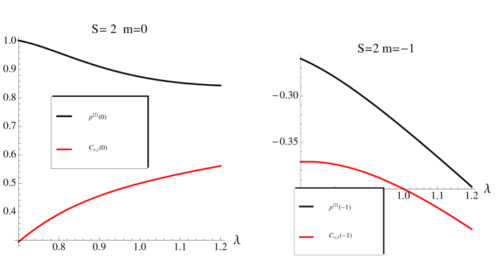
Figure 4: Two non-adiabatic corrections to Berry’s phase associated with the effective transverse magnetic field ${\Delta{\mathbf{B}}}_{\perp}(t)$ acting in the rotating frame. The first, $\phi^{(2)}_{D\perp}=\int_{0}^{T}dt\,\mu^{2}\,(\cos{\theta}\,\dot{\varphi}+\dot{\alpha})p^{(2)}(m,\lambda)$, is the modification of the dynamical phase of $\widetilde{H}(t)$ associated with ${\Delta{\mathbf{B}}}_{\perp}(t)$. The second, $\Delta^{(2)}\beta_{\perp}(\tilde{\lambda},\tilde{\mu})=\int_{0}^{T}dt\,{\tilde{\mu}}^{2}\dot{\alpha}\,{C}_{x,y}(m,\lambda)$, is Berry’s phase in the rotating frame induced by the rotation of the transverse field, ($\mu=\frac{\sin\theta\,\dot{\varphi}}{\gamma_{S}\,B},\,\widetilde{\mu}=\frac{\mu}{1-\eta}$). Note that both corrections are not geometric phases because of the presence of the factor $\mu^{2}$. The results for the cases $S=2,m=0$ and -1 are of the same order of magnitude. They can be used to make Berry’s phase determination precise at the order of $\mu^{4}$.

V.2.2 The Berry’s phase associated with $\Delta{\mathbf{B}}_{\perp}$

The full Hamiltonian $\widetilde{H}(t)=\widetilde{H}_{//}(t)+\gamma_{S}{\mathbf{S}}\cdot{\Delta{\mathbf{B}}}_{\perp}$, generates quantum cycles endowed with a non-trivial geometry since the effective transverse magnetic field ${\Delta{\mathbf{B}}}_{\perp}$ rotates about the $\hat{z}$ axis with the angular velocity $\dot{\alpha}$. As above we shall limit ourselves to the second order contribution with respect to $\mu$. We proceed by writing the eigenfunctions of $\widetilde{\cal H}(t)$ in first order expansion with respect to the parameter $\widetilde{\mu}$:

$$\hat{\psi}(m,\tilde{\lambda})-\tilde{\mu}\,\hat{\psi}^{(1)}(m,\tilde{\lambda})+\mathcal{O}(\tilde{\mu}^{2}).$$ (82)

In a way similar to what we did before, it is convenient to introduce the first order expansion of the eigenfunctions $\hat{\psi}_{x,y}(m,\lambda)$ of ${\cal H}_{x,y}(\lambda,\mu)$.

$$\hat{\psi}^{(1)}_{x,y}(m,\lambda)=\sum_{|n-m|odd}\frac{\langle\hat{\psi}(n,\lambda)|\Sigma_{x,y}|\hat{\psi}(m,\lambda)\rangle}{\mathcal{E}(m,\lambda)-\mathcal{E}(n,\lambda)}\hat{\psi}(n,\lambda).$$

By using Eq.(75), one finds that the first-order contribution to the $\widetilde{H}(t)$ eigenfunction (divided by $\tilde{\mu}$) can be written as:

$$\hat{\psi}^{(1)}(m,\tilde{\lambda})=-\cos\alpha\;\hat{\psi}^{(1)}_{x}(m,\tilde{\lambda})+\sin\alpha\;\hat{\psi}^{(1)}_{y}(m,\tilde{\lambda}).$$ (83)

It is then easily seen that Berry’s phase appears only to second order in $\mu$ and involves the familiar time derivative product: $\int_{0}^{T}dt\langle\hat{\psi}^{(1)}(m,\tilde{\lambda})|i\,\hbar\frac{\partial}{\partial t}{\hat{\psi}}^{(1)}(m,\tilde{\lambda})\rangle$, which is proportional to $\dot{\alpha}$. If the other parameters in the integrand vary slowly during the closed cycle, the only terms surviving are those proportional to $\cos^{2}\alpha$ and $\sin^{2}\alpha$ which can be replaced by their average values of 1/2. This leads to the following correction to the Berry’s phase

$$\Delta^{(2)}\beta_{\perp}(\tilde{\lambda},\tilde{\mu})=\int_{0}^{T}dt\,{\tilde{\mu}}^{2}\dot{\alpha}\,\Im\{\langle\hat{\psi}^{(1)}_{y}(m,\tilde{\lambda})|\hat{\psi}^{(1)}_{x}(m,\tilde{\lambda})\rangle\},$$ (84)

a result valid to all orders in $\eta$. It is important to note that, unlike the case of the dynamical phase (Eq. 72), this correction invoves the product of $\tilde{\mu}^{2}$ by $\dot{\alpha}$. Therefore, it is the contribution odd in $\eta$ that is eliminated by the parameter reversal, so that the dominant contribution corresponds to the limit $\eta\rightarrow 0$ i.e $\tilde{\lambda}\rightarrow\lambda\,,\,\tilde{\mu}\rightarrow\mu$. The quantity ${C}_{x,y}(m,\lambda)=\Im\{\langle\hat{\psi}^{(1)}_{y}(m,\lambda)|\hat{\psi}^{(1)}_{x}(m,\lambda)\rangle\}$ is plotted together with $p^{(2)}(m,\lambda)$ in Fig.5, leading to the same conclusions as those reached at the end of the previous paragraph.

V.3 Non-adiabatic corrections associated with ramping-up the quadratic interaction

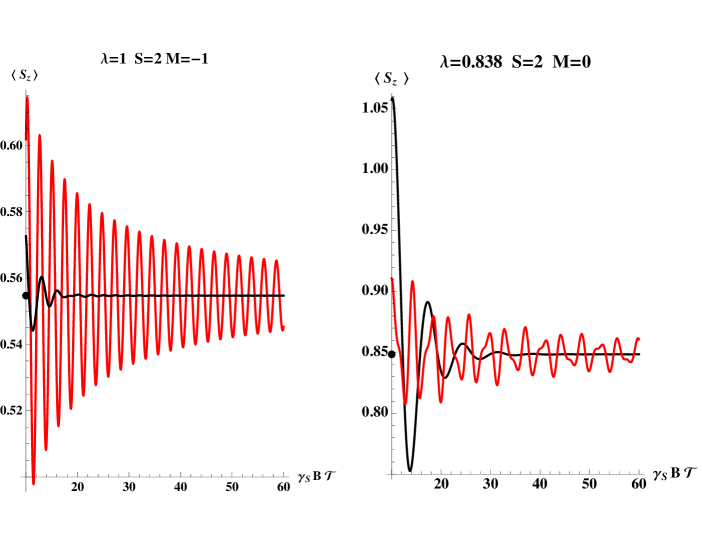
Figure 5: Effect of taming the non-adiabatic oscillations generated by a too abrupt application of the quadratic spin interaction, thanks to the use of a Blackman pulse-shaped time-derivative, oscillation taming (OT) procedure. The diagram shows non-adiabatic corrections to $\langle S_{z}\rangle$ at the end of the transition from $\lambda(0)=0$ to $\lambda(\mathcal{T})=\lambda_{0}$, starting from an initial state which is an angular momentum eigenstate $|S=2,m\rangle$ (left, $\lambda_{0}=1$, $m=-1$; right, $\lambda_{0}=\lambda^{\star}(0)=0.838$, $m=0$). The big black dot stands for the adiabatic prediction for $\langle S_{z}\rangle$. The red curves are for a linear increase of $\lambda(t)$, while the black ones correspond to the OT choice, i.e. $\dot{\lambda}(t)=f(\frac{t}{\mathcal{T}})/f(0)$, where $f(s)$ is a Blackman pulse. The rather strong oscillating non-adiabatic corrections to $\langle S_{z}\rangle$ are clearly swept away by this latter choice, provided $\gamma_{S}\,B\,\mathcal{T}\geq 25$.

In the previous subsections Berry’s phases were induced by cyclic variations of the periodic Euler angles performed in an initial state $\hat{\psi}(Sm;\lambda_{0})$. In fact to prepare this eigenstate one has to start from an eigenstate of ${\mathbf{S}}$ and $S_{z}$ at a certain time t=0. During the time interval $0\leq t\leq{\cal T}$, the evolution of the spin system is governed by ${\cal H}(\lambda(t))=S_{z}/\hbar+i\lambda(t)(S_{x}/\hbar)^{2}$. Writing $\lambda(t)=\lambda_{0}\,g(t/\cal T)$, we assume that $g(s)$ rises “slowly” from 0 to 1. We now ask asks whether, for a given values of the rising time $\cal T$, there might be a better choice for $g(s$) than just $g(s)=s$ when $\lambda_{0}\sim 1$, if one wishes to keep the non-adiabatic corrections below a predetermined level . In the present subsection, we have chosen ${1/(\gamma_{S}\,B)}$ as the time unit: all the time dependent physical quantities and their time derivatives are functions of $\tau=t\,\gamma_{S}\,B.$

V.3.1 The two-level spin system $S=2,m=\pm 1$

To get some insight into this problem, let us first consider the simple case of the adiabatic evolution of the state $S=2,\,m=\pm 1$ governed by the Hamiltonian ${\cal H}_{2}(t)={\cal H}_{odd}(2,\lambda(t))$ defined by the $2\times 2$ matrix of Eq.(29). By performing the change of variables $\zeta=\arctan{(\frac{3}{2}\lambda)}$ with $-\pi/2<\zeta<\pi/2$, one can write ${\cal H}_{2}(t)$ under the convenient form:

$${\cal H}_{2}(t)=\sec{\zeta}(\sigma_{x}\sin{\zeta}+\sigma_{z}\cos{\zeta})+\frac{5}{3}\tan(\zeta)\sigma_{0},$$ (85)

where $\sigma_{0}$ is the $2\times 2$ unit matrix and $\sigma_{x,y,z}$ are the standard Pauli matrices. We define $\Phi(2m;t)$ as the state vector obeying the Schrödinger equation relative to ${\cal H}_{2}(t)$ and satisfying the initial condition $\Phi(2m;0)=|2,m\rangle.$ We introduce the unitary rotation matrix $V_{2}(\zeta)=\exp{-i\zeta\sigma_{y}/2}$. This is the rotating frame Hamiltonian $\widetilde{\cal H}_{2}(t)$ which governs the evolution of $\widetilde{\Phi}(2m;t)=V_{2}^{-1}(\zeta)\,\Phi(2m;t)$. After some simple algebra we arrive at the familiar expressions:

$$\widetilde{\mathcal{H}}_{2}(t) = \widehat{\mathcal{H}}_{2}-i\,V_{2}(-\zeta)\frac{d}{dt}\,V_{2}(\zeta),$$ (86)

$$= \frac{5}{3}\tan(\zeta)\sigma_{0}+\sec(\zeta)\sigma_{z}-\frac{1}{2}\;\dot{\zeta}\,\sigma_{y}.$$

If $\zeta$ is assumed to grow linearly during the time interval $0\leq\tau\leq\gamma_{S}B\,{\cal T}$, $\widetilde{\mathcal{H}}_{2}(t)$ can be identified with the Hamiltonian describing a square Ramsey pulse. The same analysis can be repeated for the $S=1,m=\pm 1$. The result looks very similar : the spin dependent part of the rotating frame Hamiltonian $\widetilde{\mathcal{H}}_{1}(t)$ is formally identical, but with one significant difference, namely $\tan\zeta=/2$.

In section VI, we shall study the time evolution of a four-spin system governed by the direct sum of the two Hamiltonians: ${\widetilde{\mathcal{H}}}_{1}(t)\oplus{\widetilde{\mathcal{H}}}_{2}(t)$ relative to the same value of $\lambda$. So we will have to use the two different expressions of $\dot{\zeta}$, for S=2, $\dot{\zeta_{2}}\rightarrow 6\dot{\lambda}/(9\lambda^{2}+4)$, and for S=1, $\dot{\zeta_{1}}\rightarrow 2\dot{\lambda}/(\lambda^{2}+4)$. If $\lambda[t]$ is rising linearly, the $\dot{\zeta}[t]$ pulses are replaced by trapezoidal Ramsey pulses with sharp edges leading also to non-adiabatic oscillating corrections.

There is a standard way to wash them out which is used in nuclear magnetic resonance and atomic interferometry experiments. This consists in using the so-called Blackman pulse shape [27]. Adapted to the present context, it leads the following choice of $\dot{\lambda}(t)$:

$$\dot{\lambda}_{BM}(t) = \lambda_{0}f(\frac{t}{{\cal T}})/f(0),$$

$$\text{where}\;\;f(s) = 0.42-0.5\cos{(2\pi s)}+0.08\cos{(4\pi s)}.$$ (87)

We have solved numerically the Shrödinger equation for $\lambda_{0}=1$ for the two different choices, Blackman and trapezoidal pulses for $\dot{\lambda}(t)$. The important quantity for our purpose is $\langle S_{z}(\mathcal{T})\rangle$, since it governs the magnitude of Berry’s phase induced by the cyclic variation of the Euler-angles. It is important to note that $\langle S_{z}\rangle$ is affected to first-order in $\dot{\lambda(t)}$ in contrast with the dynamical phase which is modified only to second order.

We have plotted $\langle S_{z}(\mathcal{T})\rangle$ in Fig. 5 (left-hand curves), as function of $\gamma_{S}B\,{\cal T}$. The big (black) dot on the ordinate axis shows the adiabatic prediction. The use of the Blackman pulse for $\dot{\lambda}(t)$ leads to spectacular convergence towards the adiabatic limit: for $\gamma_{s}B\,{\cal T}\geq 25$ the non-adiabatic correction to $\langle S_{z}(\mathcal{T})\rangle$ plunges down below the 0.02 $\%$ level. We have also computed the phase shift, which is purely dynamical in the present case. As expected, the non-adiabatic corrections are much less sensitive to the time dependence of $\lambda(t)$ and we find that in both cases $|\phi_{D}(exact)-\phi_{D}(adiab)|<0.008$ when $\gamma_{S}B\mathcal{T}\geq 25$. Similar calculations for $S=|m|=1$ and the initial value $m=-1$, for $\lambda_{0}=1$ indicate that corrections (not shown) are an order of magnitude smaller.

V.3.2 More than two levels

We now extend the foregoing “rotating” frame method to non-adiabatic processes involving the mixing of more than two levels. As noted in section II.A, the Hamiltonian ${\cal H}(\lambda(t))=S_{z}/\hbar+\lambda(t)(S_{x}/\hbar)^{2}$ is described in the angular momentum basis $|S\,m\rangle$ by a real symmetric matrix. This implies that its eigenstates $\hat{\psi}(Sm;\lambda)$ can be written as real vectors. An evident consequence is the following identity, obtained by taking the derivative of the normalization condition of the real eigenvectors:

$$\langle\hat{\psi}(Sm;\lambda)|\frac{\partial}{\partial\lambda}\hat{\psi}(Sm;\lambda)\rangle=0.$$ (88)

It implies that the adiabatic phase is purely dynamical. Let us introduce now the transformation matrix:

$$V_{S}(\lambda)=\sum_{m}|\hat{\psi}(Sm;\lambda)\rangle\langle Sm|.$$ (89)

One can directly verify that $V_{S}(\lambda)$ transforms ${\cal H}(Sm;\lambda)$ into a diagonal matrix within the basis $|Sm\rangle$, by writing $V_{S}(\lambda)|Sm_{1}\rangle=\sum_{m}\hat{\psi}(Sm;\lambda)\langle Sm|Sm_{1}\rangle=\hat{\psi}(Sm_{1};\lambda).$ The time evolution in the “rotating” frame is then governed by the following Hamiltonian:

$$\widetilde{\mathcal{H}}_{S}(t) = V_{S}^{T}\,{\cal H}(Sm;\lambda)\,V_{S}-i\dot{\lambda}\,V_{S}^{T}\frac{\partial}{\partial\lambda}V_{S},$$ (90)

$$= \widehat{\mathcal{H}}_{S}(\lambda)+\Delta\widetilde{\mathcal{H}}_{S}(t).$$

The expression $\widehat{\mathcal{H}}_{S}(\lambda)=\sum_{m}\mathcal{E}(Sm;\lambda)|Sm\rangle\ \langle Sm|$ follows from eq. (89), while the identity (88) implies that $\Delta\widetilde{\mathcal{H}}_{S}(t)$ is non-diagonal:

$$\Delta\widetilde{\mathcal{H}}_{S}(t)=\sum_{m_{1}\neq m_{2}}|Sm_{2}\rangle\ \langle Sm_{1}|\times$$

$$-i\dot{\lambda}\,\langle\hat{\psi}(Sm_{1};\lambda)|\frac{\partial}{\partial\lambda}\hat{\psi}(Sm_{2};\lambda)\rangle\,.$$

By using an identity obtained from the time derivative of the eigenvalue equation (8), we can rewrite the r.h.s of the above equation as:

$$\Delta\widetilde{\mathcal{H}}_{S}(t) = -i\dot{\lambda}(t)\times\sum_{m_{1}\neq m_{2}}\frac{|Sm_{2}\rangle\ \langle Sm_{1}|}{\mathcal{E}(Sm_{1};\lambda)-\mathcal{E}(Sm_{2};\lambda)}\times$$ (91)

$$\langle\hat{\psi}(Sm_{1};\lambda)|(S_{x}/\hbar)^{2}|\hat{\psi}(Sm_{2};\lambda)\rangle\,.$$

The above formula can be considered as an adaptation of a more general one to be found in [28] and references therein. One must stress that energy denominators ${\mathcal{E}(Sm_{1};\lambda)-\mathcal{E}(Sm_{2};\lambda)}$ involve levels for which $m_{1}-m_{2}$ is even integer. For instance, in the cases $S=2,\,m=0,\pm 2$ the two energy differences involved are varying slowly within the interval $0\leq\lambda\leq\lambda_{0}=0.838.$ It follows that the time dependence of $\Delta\widetilde{\mathcal{H}}_{S}(t)$ is dominated by $-i\,\dot{\lambda}(t)\,$. Let us assume that $\lambda(t)$ is increasing linearly within the time interval $0\leq t\leq\mathcal{T}\,:\,\lambda(t)=\lambda_{0}t/T$. The effect of $\Delta\widetilde{\mathcal{H}}_{S}(t)$, as in the previous cases, is equivalent to a r.f. trapezoidal pulse with sharp edges. In the right-hand curve of Fig.5, we have plotted the average polarization as a function of the rising time $\mathcal{T}$ for $\lambda(t)$, towards the value $\lambda_{0}=\lambda^{*}(0)=0.838$. There is a a very rapid damping of the oscillating non-adabatic corrections, passing below the level of $0.2\%$ for $\gamma_{S}\,\mathcal{T}\geq 25$ when $\dot{\lambda}(t)$ has a Blackman pulse shape. This is in strong contrast with the case of a linearly rising $\lambda(t)$ where, for $\gamma_{S}\,B\mathcal{T}\geq 25$, the non adiabatic oscillating corrections have an amplitude of about $10\%$, decreasing only very slowly for longer rising times. The conspicuous chaotic behaviour in the 3-level case reflects the fact that the two frequencies involved have in general an irrational ratio.

V.4 Concluding remarks

Let us sum up the results of this last section. We have shown that if $\lambda(t)$ is a linear function within the finite time interval $0<t<T$, vanishing elsewhere, oscillating non-adiabatic corrections are generated by the sharp jumps of $\dot{\lambda}(t)$ at $t=0$ and $t=T$. We have found that the remedy is to choose for $\dot{\lambda}(t)$ a Blackman pulse shape. It is clear that one should use the same prescription for $\dot{\alpha}(t),\dot{\varphi}(t)$, for taming analogous unwanted oscillations. By solving exactly the Schrödinger equation governed by the Hamiltonian $\widetilde{H}_{//}(t)$ of Eq. (64), as illustrated in Sec. VI and in a separate paper [5] on two definite examples, we have indeed found that this remedy works beautifully.

It should be stressed that the near-degeneracies of opposite-parity level pairs $({\cal E}(m,\lambda),{\cal E}(m-1,\lambda))$, which occurs when $m>0$ and $\lambda>0$, do not affect the validity of the adiabatic approximation for Berry’s cycles if $\alpha(t)$ and $\lambda(t)$ are the only time-dependent parameters. This simplification is a consequence of the symmetry properties of the Hamiltonian $H({\mathbf{B}}(t),{\mathbf{E}}(t))$ resulting from the ${\mathbf{E}}$ and ${\mathbf{B}}$ orthogonality.

Furthermore, choosing for $\lambda(t)$ the “magic” expression $\lambda^{*}(\frac{\dot{\alpha}(t)}{\gamma_{S}\,B})$ given by Eq.(73) makes the difference of the Berry phases relative to the mirror cycles $(\alpha(t),\lambda(t))$ and $(-\alpha(t),\lambda(t))$ free of non-adiabatic corrections: all the correcting terms $\propto(\dot{\alpha}(t)/\gamma_{S}\,B)^{2q+1}$ vanish whatever $q>0$.

VI Holonomic entanglement of ${\mathbf{N}}$ non-correlated 1/2 spins

VI.1 Introduction

The purpose of this section is to show that Berry’s cycles studied is this paper are able to entangle $N$ non-correlated one-half spin states, while such an effect would not be present with linear spin couplings. Since the analysis presented here is exploratory, we shall concentrate upon the $N=4$ case which involves already the basic features of our entanglement procedure.

It is convenient to classify the set of the four states with respect to the eingenvalues of $S_{z}=\sum_{i}s_{zi}$: $M=\sum_{i=1}^{4}m_{i}$. The case $M=2$ is trivial. The case $M=1$ is the most interesting one for our purpose and will be the main subject of this paper. The case $M=0$ will be discussed briefly at the end of this section. The results for negative values of $M$ are readily obtained from the positive ones by using the reflection laws introduced in section III. The vector space generated by the linear combinations of non-correlated spin states with $M=1$ has a dimension four and the natural choice for a basis is the set of the four orthogonal states:

$$\Phi^{(1)} = |-\frac{1}{2}\rangle\otimes|\frac{1}{2}\rangle\otimes|\frac{1}{2}\rangle\otimes|\frac{1}{2}\rangle,$$

$$\Phi^{(2)} = |\frac{1}{2}\rangle\otimes|-\frac{1}{2}\rangle\otimes|\frac{1}{2}\rangle\otimes|\frac{1}{2}\rangle,$$

$$\Phi^{(3)} = |\frac{1}{2}\rangle\otimes|\frac{1}{2}\rangle\otimes|-\frac{1}{2}\rangle\otimes|\frac{1}{2}\rangle,$$

$$\Phi^{(4)} = |\frac{1}{2}\rangle\otimes|\frac{1}{2}\rangle\otimes|\frac{1}{2}\rangle\otimes|-\frac{1}{2}\rangle.$$ (92)

We shall assume that the time evolution of the four-spin state $\Psi_{4}(t)$ is governed by the time-dependent Hamiltonian $H_{N}(t)=H({\mathbf{B}}(t),{\mathbf{E}}(t))$, which looks formally like the quadratic spin Hamiltonian of Eq.(1) discussed extensively in the present paper:

$$H({\mathbf{B}}(t),{\mathbf{E}}(t)) = U(R(t))\,\hat{H}(B(t),E(t))\,U^{-1}(R(t)),$$

$$\hat{H}(B(t),E(t)) = \gamma_{S}\,B(t)(S_{z}/\hbar+\lambda(t)(S_{x}/\hbar^{)}2).$$

The crucial difference lies in the fact that ${\mathbf{S}}$ is meant to be the total spin operator ${\mathbf{S}}=\sum_{i=1}^{N}{\mathbf{s}}_{i}$.

We shall take as initial state for $\Psi_{4}(t)$, one of the non-corellated states appearing in equation (92), say, $\Psi_{4}(0)=\Phi^{(1)}$. By expanding $H_{N}(t)$ in terms of single-spin operators one gets a sum of spin-spin interactions: $\propto{\mathbf{s}}_{i}\cdot\hat{n}\;\;{\mathbf{s}}_{j}\cdot\hat{n}$. where $\hat{n}$ is given by $\hat{n}=U(R(t))\hat{x}$. This indicates that $H_{N}(t)$ can create spin correlations in the state $\Psi_{4}(t)$. As a final remark, we stress that, by construction, $H_{4}(t)$ is invariant under all permutations of the $N=4$ spins. This invariance property will play an essential role in our entanglement procedure.

VI.2 Expansion of a non-correlated four spin state into a sum of the ${\mathbf{S}}^{2}$ eigenstates

As a first step, we shall construct four angular momentum eigenstates which are linear combinations of the four states $\Phi^{(i)}$. Using the rules of adddition of quantum angular momenta, one finds that the possible eigenvalues of ${{\mathbf{S}}}^{2}$ , $\hbar^{2}S(S+1)$, correspond to $S=2$ and $S=1$. There is a unique way to construct the state $S=2$. It is obtained by applying the operator $S_{-}=S_{x}-iS_{y}$ upon the state $S=2,M=2$ i.e. $\Psi_{2\;2}=|\frac{1}{2}\rangle\otimes|\frac{1}{2}\rangle\otimes|\frac{1}{2}\rangle\otimes|\frac{1}{2}\rangle$. One gets immediately:

$$\Psi_{2\,1}=\frac{1}{2}(\Phi^{(1)}+\Phi^{(2)}+\Phi^{(3)}+\Phi^{(4)}).$$ (93)

The above state is clearly invariant under all permuations of the 4-spin states.

One must now construct three orthogonal states with $S=M=1,\Psi^{i}_{\,1\;1}$ which will have different symmetry under the permutations of the four spins. If one ignores the orthogonal condition, it is easy to get three $S=1$ states which are linearly independent. The method consists in taking a linear combination of 2 states $\Phi^{(i)}$ in such a way as to factor out the two spin singlet state: $(|\frac{1}{2}\rangle\otimes|-\frac{1}{2}\rangle-|-\frac{1}{2}\rangle\otimes|\frac{1}{2}\rangle)/\sqrt{2}$, which is invariant under the rotation group. Let us give a typical example of such a construction:

$$\Phi^{(1,2)} = (\Phi^{(1)}-\Phi^{(2)})/\sqrt{2},$$

$$= \frac{1}{\sqrt{2}}\left(|\frac{1}{2}\rangle\otimes|-\frac{1}{2}\rangle-|-\frac{1}{2}\rangle\otimes|\frac{1}{2}\rangle\right)\otimes|\frac{1}{2}\rangle\otimes|\frac{1}{2}\rangle$$

is a good candidate for a $S=M=1$ state. Two similar $S=M=1$ states $\Phi^{(1,3)},\Phi^{(1,4)}$ are obtained from $\Phi^{(1,2)}$ by performing the cyclic permutation $(234)$. These three states are linearly independent but a basis with orthogonal states would be more convenient. Since symmetry will be the basic tool in this subsection, let us start with the more symmetric $S=M=1$ state : $\frac{1}{2}(\Phi^{(1)}-\Phi^{(2)}+\Phi^{(3)}-\Phi^{(4)})$. The two other states are obtained by applying the cyclic permutation (234). One arrives then to the following basis for the $S=M=1$ subspace, easily seen to be orthogonal:

$$\Psi^{1}_{\,1\;1} = \frac{1}{2}(\Phi^{(1)}-\Phi^{(2)}+\Phi^{(3)}-\Phi^{(4)}),$$

$$\Psi^{2}_{\,1\;1} = \frac{1}{2}(\Phi^{(1)}-\Phi^{(3)}+\Phi^{(4)}-\Phi^{(2)}),$$

$$\Psi^{3}_{\,1\;1} = \frac{1}{2}(\Phi^{(1)}-\Phi^{(4)}+\Phi^{(2)}-\Phi^{(3)}).$$ (95)

The three above states have, different symmetry properties under the three permutations (23), (24), (34), which are listed below:

$$\{(23),(24),(34)\}\Psi^{1}_{\,1\;1} = \{-1,\,1,\,-1\}\Psi^{1}_{\,1\;1},$$

$$\{(23),(24),(34)\}\Psi^{2}_{\,1\;1} = \{\;1,\,-1,\;1\;\}\Psi^{2}_{\,1\;1},$$

$$\{(23),(24),(34)\}\Psi^{3}_{\,1\;1} = \{-1,-1,\,1\,\}\Psi^{3}_{\,1\;1}.$$

The four eigenstates $\Psi^{i}_{\,1\;1}$ and $\Psi_{\,2\;1}$ constitute a complete ortho-normal basis for the four spin one-half states with $M=1$. The expansion of the four non-corrrelated states $\Phi^{(i)}$ are readily obtained from equations (92) and (93)

$$\Phi^{(i)} = \frac{1}{2}\left(\sum_{j=1}^{j=3}a_{i\,j}\,\Psi^{j}_{\,1\;1}+\Psi_{2\,1}\right),\;\;{\rm with}$$ (96)

$$a_{1\,j} = \{1,1,1\},\;\;\;\;\;\;a_{2\,j}=\{-1,-1,1\},$$

$$a_{3\,j} = \{1,-1,-1\},\,a_{4\,j}=\{-1,1,-1\}.$$ (97)

VI.3 The adiabatic evolution of four non-correlated, 1/2 spin states governed by $H({\mathbf{B}}(t),{\mathbf{E}}(t))$

The Hamiltonian $H_{4}(t)=H({\mathbf{B}}(t),{\mathbf{E}}(t))$, as noted before, is invariant under either one of the three “parities” $\epsilon_{(23)},\epsilon_{(24)},\epsilon_{(34)}$, associated with the permutations (23),(24) and (34). As a consequence, the matrix elements: $\langle\Psi^{i}_{\,1\;M}|H_{4}(t)|\Psi^{j}_{\,1\;M^{\prime}}\rangle$ for $M=M^{\prime}=1$ vanish if $i\neq j$ . Moreover, the same result holds if $M=\pm 1$, $M^{\prime}=\pm 1$ and $M\neq M^{\prime}$, since the lowering operator $S_{x}-iS_{y}$ commutes with all the four spin permutations. Using the same symmetry arguments, one sees immediately that the matrix elements $\langle\Psi_{\,2\;M}|H_{4}(t)|\Psi^{i}_{\,1\;M^{\prime}}\rangle$ vanish whatever the values of $i,\,M,\,M^{\prime}$. If $U_{4}(t)$ stands for the unitary operator associated with the quantum evolution governed by $H_{4}(t)$, the four states $U_{4}(t)\Psi_{2\;M}$, and and $U_{4}(t)\Psi^{i}_{1\;M^{\prime}}$ will have the same permutation symmetries as their parent states. In conclusion, the four states $\Psi_{2\,M},\Psi^{i}_{1\,M^{\prime}}$ behave vis à vis the Hamiltonian $H_{4}(t)$, as if they were associated with isolated spins S and we can apply to them the results derived in the previous sections.

Our Berry’s cycle is organized in three steps. At $t$=0, $H_{4}(0)=\gamma_{S}\,B(t)S_{z}$. The first step $0\leq t\leq{\cal T}$ involves the adiabatic ramping of $\lambda(t)$ from 0 to $\lambda_{0}\simeq-1$. In the second step ${\cal T}\leq t\leq 3{\cal T}$, one proceeds to the rotation of ${\mathbf{E}}$ around ${\mathbf{B}}$ by an angle 3$\pi$, while keeping $\lambda(t)=\lambda_{0}$. For the third step, $3{\cal T}\leq t\leq 4{\cal T}$, $\lambda(t)$ makes an adiabatic return to its initial value $\lambda=0$. During the whole cycle the time dependences of $\dot{\lambda}(t)$ and $\dot{\alpha}(t)$ are described by Blackman functions. The effect of this choice is to tame the non-adiabatic oscillating corrections which would be generated, if these parameters had discontinuous time-derivatives.

We have performed an exact theoretical analysis of the cycle by solving the corresponding Schrödinger equation in the rotating frame with $\gamma_{s}B{\cal T}=25$. We have found that the adiabatic approximation is working to better than 0.1$\%$. It turns out that somewhat accidentally the difference of the dynamical phases for $S=2,M=1$ and $S=1,M=1$ is close to 0 modulo 2$\pi$. Slightly tuning the $\lambda$-rising (-lowering) times can improve the cancellation to the 0.1$\%$ level. The cyclic evolution of the four spins, initially non-correlated, appears then as completely governed by the Berry’s phases $\beta(2,1;\lambda_{0})$ and $\beta(1,1;\lambda_{0})$.

VI.4 The final construction of the four-spin holonomic entangled state

At the end of the Berry’s cycle, $\Phi^{(i)}$ is transformed into the following state:

$$\Phi^{(i)}_{BP}(\lambda_{0}) = \frac{1}{2}\{\exp(i\,\beta(2\,1;\lambda_{0}))\,\Psi_{2\,1}+$$ (98)

$$\exp(\,i\,\beta(1\,1;\lambda_{0}))\sum_{j=1}^{j=3}a_{i\,j}\,\Psi^{j}_{\,1\;1}\}.$$

Using Eq.(96) to express the sum $\sum_{j=1}^{j=3}a_{i\,j}\,\Psi^{j}_{\,1\;1}$ in terms of $\Phi^{(i)}$ and $\Psi_{2\,1}$, one obtains the final expression:

$$\Phi^{(1)}_{BP}(\lambda_{0}) = \exp\left(\,i\,\beta(1\,1;\lambda_{0})\right)\left(\Phi^{(1)}-\frac{1}{2}\Psi_{2\,1}\right)+$$ (99)

$$\frac{1}{2}\exp\left(\,i\,\beta(2\,1;\lambda_{0})\right)\Psi_{2\,1}.$$

(We can verify on this expression that if $\Delta\beta(\lambda_{0})=\beta(2\,1;\lambda_{0})-\beta(1\,1;\lambda_{0})=0$, then $\Phi^{(1)}_{BP}$ coincides with $\Phi^{(1)}$ up to a phase, as one expects).

From the energy curves given in Fig.1 one sees that the region $\lambda>0$ should be, in principle avoided, since the nearly crossing levels $S=2,M=2$ and $S=2,M=1$ could spoil the validity of the adiabatic approximation, while the region $\lambda<0$ is much more favourable. However, in the present context where $\lambda$ and $\alpha$ are the only time-dependent parameters, this is only a protection against stray magnetic fields orthogonal to the main field, since $H_{4}(t)$ has no $\Delta M=\pm 1$ matrix elements. The two Berry’s phases are given explicitly by rather simple expressions:

$$\beta(2\,1;\lambda_{0}) = 3\pi\left(\frac{2}{\sqrt{9\lambda_{0}^{2}+4}}-1\right),$$

$$\beta(1\,1;\lambda_{0}) = 3\pi\left(\frac{2}{\sqrt{\lambda_{0}^{2}+4}}-1\right).$$ (100)

In order to obtain the maximum entanglement of $\Phi^{(i)}_{BP}$ after a rotation of $3\pi$, it is interesting to choose $\lambda_{0}=\lambda_{max}=-0.97$ which leads to $\Delta\beta(\lambda_{max})=-\pi$. Replacing $\Psi_{2\,1}$ by its expression in terms of $\Phi^{(i)}$ ( Eq.(93)) we arrive at the final expression of the four quantum entangled states, generated by the Berry’s cycles with $\Delta\beta(\lambda_{0})=-\pi$, from any of the four non-correlated states with M=1 listed in equation ( 92 )

$$\Phi^{i}_{BP}(\lambda_{max})=\exp(i\chi)\left(\Phi^{(i)}-\frac{1}{2}\sum_{j=1}^{4}\,\,\Phi^{(j)}\right),$$ (101)

where $\chi=\beta(1\,1;\lambda_{max})$. In order to make more apparent the holonomic entanglement resulting from the Berry cycle, let us rewrite $\Phi^{1}_{BP}(\lambda_{max})$, using the explicit forms of the non-correlated states $\Phi^{(i)}$ given in Eq. (92):

$$\Phi^{(1)}_{BP}(\lambda_{max}) = \frac{\exp(i\chi)}{2}\,(\,|-\frac{1}{2}\rangle\otimes|\frac{1}{2}\rangle\otimes|\frac{1}{2}\rangle\otimes|\frac{1}{2}\rangle$$ (102)

$$-|\frac{1}{2}\rangle\otimes|-\frac{1}{2}\rangle\otimes|\frac{1}{2}\rangle\otimes|\frac{1}{2}\rangle$$

$$-|\frac{1}{2}\rangle\otimes|\frac{1}{2}\rangle\otimes|-\frac{1}{2}\rangle\otimes|\frac{1}{2}\rangle$$

$$-|\frac{1}{2}\rangle\otimes|\frac{1}{2}\rangle\otimes|\frac{1}{2}\rangle\otimes|-\frac{1}{2}\rangle\,).$$

A similar approach can be used to treat the case of four non-correlated spins with $M=\sum_{i=1}^{4}m_{i}=0$. Among the three angular momentum states $S=2,1,0;M=0$, only the state $S=2,M=0$ has a non-vanishing Berry’s Phase. As a consequence, one gets an entanglement which is weaker than in the above $M=1$ case where it is maximum. The case of 8 one-half spins (or 8 Qbits) with $M=1$ is of particular interest since it involves four non-vanishing Berry’s Phases for $S=1,2,3,4$ but it will require more powerful Group Theory tools, like the Young Operators [30]. However, the basic ideas of the entanglement procedure would remain the same.

The reader might have the impression that the above method of entanglement is constrained by the fact that Berry’s phases depend upon few parameters. However one should keep in mind that $\beta(SM;\lambda)$ is actually given by a Bohm-Aharonov integral involving an Abelian gauge field along a closed loop drawn upon the four-dimension manifold ${\mathbf{C}}P^{2}$, which implies a considerable freedom (see Eq. (57)).

From a practical point of view entanglement methods based on geometric phases are known to present advantages of robustness: they are resilient to certain types of errors in the control of the parameters driving the quantum evolution [11].

We end this section by giving an example where the collective spin-spin interaction between a few spins, similar to that described by $H_{N}(t)$, has been successively implemented. This concerns the case of two or four alkali-like ions, without nuclear spin, in an ion-trap. The idea is to realize illumination of the N ions (N Qbits) with two lasers fields having two different frequencies so that the two-photon process, exciting any pair of ions in the trap is resonant, but neither of the frequencies are resonant with single excitation of an ion [31, 32]. Realization performed for two and four ions in a trap [33], can be generalized to more ions. In the present context it would be necessary to match the magnitude of the dc magnetic field and the radiation fields. According to the analysis given above, rotating the linear polarization of the radiation fields around the ${\mathbf{B}}$-field should make it possible to generate holonomic entanglement of the Qbits.

VII Summary and perspectives

VII.1 Synopsis of the paper

The purpose of this paper is the theoretical study of the Berry’s phases, generated in cyclic evolutions of isolated spins of arbitrary values. The spins are assumed to be non-linearly coupled to time-dependent external electromagnetic fields (possibly effective) via the superposition of a dipole and a quadrupole couplings. Configurations leading to degenerate instantaneous eigenvalues are avoided. In other words non-Abelian Berry’s phases are not considered. We also assume that the two effective fields are orthogonal, a mild restriction but with many advantages. This implies several discrete symmetries of the spin Hamiltonian which simplify considerably the algebra. For instance, two angular momentum states having different quantum numbers $m_{1}$ and $m_{2}$ are coupled if, and only if, $m_{1}-m_{2}$ is an even integer. Furthermore, for $S=1$, the geometric space of the Hamiltonian parameters is isomorphic to the density matrix space ${\mathbf{C}}P^{2}$ which makes the Berry’s and Aharonov-Anandan geometric phases mathematically identical.

Using rotation group theory, and the aforementioned discrete symmetries, we obtain compact expressions for the instantaneous eigenfunctions of the Hamiltonian, labelled by the magnetic quantum number $m$, valid in the limit of small quadrupole coupling.

We derive an explicit compact expression for the Berry’s phase $\beta(m)$ in terms of the usual Euler angles $\varphi,\theta,\alpha$ associated with the trihedron defined by the ${\mathbf{B}},{\mathbf{E}}$ directions, and an extra dimensionless parameter $\lambda$ giving the quadrupole to dipole coupling ratio. The result is given as a loop integral of an Abelian field along a closed circuit drawn upon the parameter space ${\mathbf{C}}P^{2}$,

$$\beta(m)=\oint_{{\cal C}}p(m,\lambda)(\cos\theta\,d\varphi+d\alpha)-m\,(d\varphi+d\alpha).$$

where $\hbar\,p(m,\lambda)$, the average value of the spin angular momentum taken along the ${\mathbf{B}}$ field, is just the gradient of the eigenenergy with respect to ${\mathbf{B}}$. The apparent simplicity of the above formula conceals the geometry contained in $p(m,\lambda)$. This important feature is clearly exhibited in Berry’s cycles where $\lambda$ and $\alpha$ are the sole varying parameters. The case $S=2,m=0$, where the Berry’s Phase is vanishing for a linear spin Hamiltonian, is particularly spectacular: $p(0,\lambda)$ is an odd function of $\lambda$ and takes the value 1 when $\lambda=1$. This peculiar geometry is best illustrated in Fig. 2 where $A_{\alpha}=p(0,\lambda)$ is plotted against the spherical coordinate $\tilde{\theta}$ defined by $\lambda=-2\cot\tilde{\theta}$ with $0<\tilde{\theta}<\pi$.

The non adiabatic corrections associated with the Euler angles derivatives have been analyzed within the rotating frame attached to the time-varying fields. The Coriolis effect generates an extra magnetic field $\Delta{\mathbf{B}}$ which involves a linear combination of the Euler-angle time derivatives. The longitudinal component along the ${\mathbf{B}}$ field is the only one which survives when $\alpha$ is the sole time-dependent Euler angle. The corresponding Hamiltonian $\widetilde{H}_{//}$ is devoid of any geometry. As a consequence, the phase shift acquired at the end of the cycle $\tilde{\phi}({\mathbf{B}}+\Delta{\mathbf{B}})$ is purely dynamical. The Berry’s phase is incorporated into the dynamical phase under the form of its first-order contribution with respect to $\eta=-\Delta B_{//}/B=(\cos{\theta}\;\dot{\varphi}+\dot{\alpha})/(\gamma_{S}B)$. The higher-order terms give all the non-adiabatic corrections associated with $\dot{\alpha}$ when it is the only varying periodic parameter. We have also shown that the subset of these corrections, odd under a reversal of $\eta$, cancel exactly for “magic” values $\lambda=\lambda^{*}(\eta)$. This cancellation is implemented in the experimental project described in reference [5]. The case of the non-adiabatic corrections induced by the transverse magnetic field $\Delta B_{\perp}/B$ is somewhat more involved since it introduces a non-trivial geometry and, as a consequence, a Berry’s phase contribution to be added to the one coming from the transverse dynamical phase. An explicit evaluation of the complete lowest-order total correction $\Delta\beta_{\perp}/\beta$ is found to be $\propto(\dot{\varphi}/\gamma_{S}B)^{2}$ up to a numerical coefficient computed explicitly for $S=2,\,m=0,$ and -1. The results are displayed in Fig. 4.

This discussion hinges upon the implicit assumption that the finite value of $\lambda$ is reached by an adiabatic ramping governed by $\mathcal{H}(\lambda(t))=S_{z}/\hbar+\lambda(t)(S_{x}/\hbar)^{2}$, leading to a pure eigen-state $\hat{\psi}(\lambda)$, free of any non-adiabatic pollution. To analyse this problem, it was convenient to perform the time dependent unitary transformation $V(\lambda(t))$ which transform $\mathcal{H}(\lambda(t))$, into a diagonal matrix within the angular momentum basis. It follows from the symmetry properties of $\mathcal{H}(\lambda(t))$ that $V(\lambda(t))$ can be taken as real and symmetric. The Hamiltonian, which governs the spin evolution in the transformed basis, contains the non-diagonal term $i\dot{\lambda}(t)V^{T}(\lambda(t))\frac{\partial}{\partial\lambda}V(\lambda(t))$. Since its time dependence is dominated by the time derivative $\dot{\lambda}(t)$, a linear increase of $\lambda(t)$ would be equivalent to a rf pulse with sharp edges leading to the oscillating non-adiabatic corrections exhibited in Fig.5. The standard procedure to smooth them out is to use for $\dot{\lambda}(t)$ a Blackman pulse shape [27]. The efficiency of the procedure for taming the non-adiabatic oscillations is clearly exhibited in Fig.5. There is a second assumption implicit in the rotating frame analysis, namely that the adiabatic approximation be valid for the rotating frame Hamiltonian $\widetilde{H}(t)$. By solving numerically the Shrödinger equation describing the whole cycle, we have verified (see ref. [5] for explicit numerical results) that, indeed, the adiabatic approximation works beautifully provided one also uses a Blackman-pulse shape for the angular speed, $\dot{\alpha}(t)$.

In the last section, we propose a procedure to entangle a system of N non-correlated one-half spins (or N Qbits). It involves Berry’s cycles generated by an Hamiltonian formally identical to one given in equation (1), but with an important change: ${\mathbf{S}}$ stands now for the total spin operator ${\mathbf{S}}=\sum_{i=1}^{N}{\mathbf{s}}_{i}$. We have used a method which is well adapted, to the simple configuration of four one-half spins. In view of possible extensions to $N$ spins with $N>4$, we would like to rephrase our approach within a more general framework. A configuration of $N$ non-correlated $\frac{1}{2}$-spins can be described by a factorizable spin tensor of order $N$. It constitutes a reducible representation of the $S(U_{2})$ group. There is a general procedure to decompose this tensor into irreducible tensors, associated with eigenstates of ${\mathbf{S}}^{2}$ and $S_{z}$. With the exception of the trivial case $N=2$, the angular momentum state $\Psi_{S\,M}$ can appear several times in the decomposition. According to a known theorem of Group Theory [30], all the states $\Psi_{S\,M}^{i}$ have different symmetry properties under the permutation of the $N$ spins and they can be organized into an orthogonal basis, $\langle\Psi_{S\,M}^{i}|\Psi_{S^{\prime}\,M^{\prime}}^{j}\rangle=\delta_{S,S^{\prime}}\delta_{M,M^{\prime}}\delta_{i,j}$. Let us now consider the set of Hamiltonians ${\cal{H}}({\mathbf{S}})$ which are given by a non-linear series expansion with respect to the spin components $S_{x,y,z}$. By construction, ${\cal{H}}({\mathbf{S}})$ is invariant upon any permutation of the $N$ spins. As a consequence, ${\cal{H}}({\mathbf{S}})$ is diagonal within the basis $\Psi_{S\,M}^{i}$: $\langle\Psi_{S\,M}^{i}|{\cal{H}}({\mathbf{S}},t)|\Psi_{S^{\prime}\,M^{\prime}}^{j}\rangle=\delta_{S,S^{\prime}}\delta_{i,j}\langle\Psi_{S\,M}^{i}|{\cal{H}}({\mathbf{S}},t)|\Psi_{S,M^{\prime}}^{i}\rangle.$ The above equation expresses the simple fact that ${\cal{H}}({\mathbf{S}})$ is acting upon the states $\Psi_{S\,M}^{i}$ as if they were isolated spins $S$. Any initial state of $N$ non-correlated spins can then be written as $|\Psi_{N}(t=0)\rangle=\sum_{i\,,S}a_{S\,M}^{i}|\Psi_{S\,M}^{i}\rangle.$ One performs now an adiabatic Berry’s cycle along a closed loop in the parameter space such that ${\cal{H}}({\mathbf{S}},0)={\cal{H}}({\mathbf{S}},T)=\gamma_{S}{\mathbf{S}}\cdot{\mathbf{B}}$. At the end of the cycle the $N$ spin system is given by the following state vector: $|\Psi_{N}(T)\rangle=\sum_{i,\,S}a_{S\,M}^{i}\exp{i\beta(S\,M)}|\Psi_{S,\,M}^{i}\rangle.$

With a suitable choice of the Berry’s cycle, we have shown in the particular case $N=4,M=1$ that the final state is endowed with a maximal entanglement. Thus extension to higher values of $N$ is worth pursuing, remembering that according to quantum computing experts: “entanglement, as with most good things, it is best consumed in moderation” [34].

VII.2 Experimental perspectives

In a separate work, we have explored the possibility of cold alkali atoms in their ground state to measure Berry’s phase with atomic interferometers. The spin operator is then identified with the total angular momentum ${\mathbf{F}}={\mathbf{s}}+{\mathbf{I}}$. The ac-Stark shift induced by a linearly polarized light beam tuned off-resonance of one resonance line, can induce the quadratic interaction if one accepts a few experimental compromises. The candidate for our spin system is the ground state hyperfine (hf) level $5S_{1/2},\,F=2$ of ⁸⁷Rb. We have found judicious to tune the laser frequency midway between the two lines $5S_{1/2},\,F=2\rightarrow 5P_{1/2},\,F=1$, and $F=2$ . The effective quadrupole coupling takes then the simple form: $H_{Q}=\frac{\hbar\Omega^{2}}{\Delta{\mathcal{W}}_{P}}({\mathbf{F}}\cdot\hat{e})^{2},$ where $\Delta{\mathcal{W}}_{P}$ is the $5P_{1/2}$ hf splitting, $\Omega$ the Rabi frequency relative to the transition $5S_{1/2}\rightarrow 5P_{1/2}$ and $\hat{e}$ the light polarization. However there is a certain price to be paid arising from the instability of the “dressed” ground state depicted by its decay rate $\Gamma_{dec}=\frac{4\Omega^{2}}{\Delta{\mathcal{W}}_{P}^{2}}\Gamma_{5P_{1/2}}$ (where $\Gamma_{5P_{1/2}}$ is the spontaneous decay rate of the excited state). Although, with our choice of detunings, this effect does not affect the Berry phase value, it can perturb seriously the measurement process. One is clearly facing a difficult optimization problem, if one wants also to keep the non-adiabatic correction below the $0.1\%$ level. We give here some features of the solution described in ref. [5]. With an external magnetic field of 1 mG, one can adjust $\Omega^{2}$ (i.e. the light beam intensity) in order to get a quadrupole to dipole couplings ratio close to 1. The off-diagonal density matrix element holding the Berry Phase, decays to half its initial value. But adjusting the interferometer parameters can compensate for this effect and keep the interference contrast close to its maximum.

On the above example the role of both the hyperfine interaction, and the instability of the atomic excited states is clearly exhibited. This gives a clear illustration of the atomic internal structure contribution to the spin dynamics. Although these effects upon Berry’s cycles can be accounted for by choosing appropriate values of the effective ${\mathbf{B}},{\mathbf{E}}$ fields, they lead to severe experimental constraints. It looks possible to satisfy these constraints with ⁸⁷Rb atoms but with light alkalis this is far from obvious [5]. On the other hand, the external degrees of freedom, i.e. the atomic nuclei coordinates have been supposed fixed physical quantities, an assumption which would obviously fail for ultra cold atoms belonging to a fermionic or bosonic quantum gas. In such a case, these coordinates become truly quantum variables which appear explicitly in the density matrix of the system. The problem of Berry’s phase generated by an adiabatic cycle of the coupled external fields is well beyond the scope of the present paper.

Acknowledgments

The authors thank Dr. M. D. Plimmer for helpful discussions.

Appendix. Some useful formulas and algebraic results for S=3 and S=4.

$${\cal H}_{odd}(3,\lambda)=\left(\begin{array}[]{cccc}\frac{3\lambda}{2}+3&\frac{\sqrt{15}\lambda}{2}&0&0\\ \frac{\sqrt{15}\lambda}{2}&\frac{11\lambda}{2}+1&3\lambda&0\\ 0&3\lambda&\frac{11\lambda}{2}-1&\frac{\sqrt{15}\lambda}{2}\\ 0&0&\frac{\sqrt{15}\lambda}{2}&\frac{3\lambda}{2}-3\end{array}\right)$$ (103)

$${\cal H}_{even}(3,\lambda)=\left(\begin{array}[]{ccc}4\lambda+2&\sqrt{\frac{15}{2}}\lambda&0\\ \sqrt{\frac{15}{2}}\lambda&6\lambda&\sqrt{\frac{15}{2}}\lambda\\ 0&\sqrt{\frac{15}{2}}\lambda&4\lambda-2\end{array}\right)$$ (104)

$$\det({\cal H}_{odd}(3,\lambda)-x\;\mathbf{l})=x^{4}-14x^{3}\lambda+49x^{2}\lambda^{2}-10x^{2}-36x\lambda^{3}+102x\lambda-216\lambda^{2}+9,$$ (105)

$$\det({\cal H}_{even}(3,\lambda)-x\;\mathbf{l})=x^{3}-14x^{2}\lambda+49x\lambda^{2}-4x-36\lambda^{3}+24\lambda.$$ (106)

$${\cal H}_{even}(4,\lambda)=\left(\begin{array}[]{ccccc}2\lambda+4&\sqrt{7}\lambda&0&0&0\\ \sqrt{7}\lambda&8\lambda+2&3\sqrt{\frac{5}{2}}\lambda&0&0\\ 0&3\sqrt{\frac{5}{2}}\lambda&10\lambda&3\sqrt{\frac{5}{2}}\lambda&0\\ 0&0&3\sqrt{\frac{5}{2}}\lambda&8\lambda-2&\sqrt{7}\lambda\\ 0&0&0&\sqrt{7}\lambda&2\lambda-4\end{array}\right)$$ (107)

$${\cal H}_{odd}(4,\lambda)=\left(\begin{array}[]{cccc}\frac{11\lambda}{2}+3&\frac{3\sqrt{7}\lambda}{2}&0&0\\ \frac{3\sqrt{7}\lambda}{2}&\frac{19\lambda}{2}+1&5\lambda&0\\ 0&5\lambda&\frac{19\lambda}{2}-1&\frac{3\sqrt{7}\lambda}{2}\\ 0&0&\frac{3\sqrt{7}\lambda}{2}&\frac{11\lambda}{2}-3\end{array}\right)$$ (108)

$$\det({\cal H}_{even}(4,\lambda)-x\;\mathbf{l}) = x^{5}-30x^{4}\lambda+273x^{3}\lambda^{2}-20x^{3}-820x^{2}\lambda^{3}+472x^{2}\lambda,$$ (109)

$$\det({\cal H}_{odd}(4,\lambda)-x\;\mathbf{l})=x^{4}-30x^{3}\lambda+273x^{2}\lambda^{2}-10x^{2}-820x\lambda^{3}+182x\lambda+576\lambda^{4}-712\lambda^{2}+9.$$ (110)

References

- [1] M.V. Berry, Proc. R. Lond. A392, 45 (1984).
- [2] B. Simon, Phys. Rev. Lett. 51, 2167 (1983).
- [3] Y. Aharonov and J. Anandan, Phys. Rev. Lett. 58, 1593 (1987).
- [4] N. F. Ramsey, Phys. Rev. 76, 996L. and Molecular Beams (Clarendon, Oxford, UK, 1956), pp. 124-133 (1949).
- [5] M.A. Bouchiat and C. Bouchiat, to be published.
- [6] A. Shapere and F. Wilczek, Geometric Berry’s Phases in Physics, Advanced Series in Mathematical Physics, Vol. 5 (World Scientific, Singapore) (1989).
- [7] J. Anandan, J. Christian and K. Wanelik, Resource letter GPP-1 Geometric phases in physics, Am. J. Phys. 65, 180 (1997).
- [8] M. Berry, Sci. Am. 259, 46 (1988).
- [9] Holstein, J. Am. Phys. 57, 1079 (1989).
- [10] J. Zwanziger, M. Koenig and A. Pines, Ann. Rev. Phys. Chem. 41, 601 (1990).
- [11] E. Sjöqvist, Physics1, 35 (2008).
- [12] J. A. Jones, V. Vedral, A. Ekert, and G. Castagnoli, Nature 403, 869 (2000).
- [13] E.D. Commins, Am. J. Phys. 59, 1077 (1991).
- [14] M. Pendlebury et al., Phys. Rev. A 70, 032102 (2004).
- [15] M.R. Tarbutt, J.J. Hudson, B.E. Sauer, E.A. Hinds, Faraday Discuss. 142, 37 (2009).
- [16] T. Bergmann, T. Gasenzer, O. Nachtmann, Eur. Phys. J. D 45, 197 and 211 (2007).
- [17] DeKieviet et al., 2010, e-print arXiv:physics.atom-ph/1003.0622.
- [18] R. Tycko, Phys. Rev. Lett. 58, 2281 (1987).
- [19] J.W. Zwanziger, M. Koenig and A. Pines, Phys. Rev. A 42, 3107 (1990).
- [20] F. Wilczek and A. Zee, Phys. Rev. Lett., 58, 2111 (1984).
- [21] E. Kiritsis, Commun. Math. Phys. 111, 417 (1987).
- [22] A. Zee, Phys. Rev. A 38, 1 (1988).
- [23] C. Cohen Tannoudji and J. Dupont-Roc, Phys. Rev. A 5, 968 (1972).
- [24] C. Bouchiat and G. W. Gibbons, J. Phys. France 49, 187 (1988).
- [25] C. Bouchiat, J. Phys. France 50, 1041 (1989).
- [26] L.I Schiff, Quantum Mechanics, 2nd ed., Sec. 31 (MacGraw-Hill, New-York, 1955).
- [27] F. J. Harris, Proc. IEEE, 66, 51 (1978).
- [28] M.V. Berry, Proc. R. Soc. Lond. A 414, 31 (1987).
- [29] Y. Aharonov and D. Bohm, Phys. Rev. 115, 485 (1959).
- [30] M. Hamermesh, 1962, Group Theory, (Pergamon).
- [31] K. Molmer and A. Sorensen, Phys. Rev. Lett. 82, 1835 (1999).
- [32] A. Sorensen and A. Molmer, Phys. Rev. Lett. 82, 1971 (1999).
- [33] C.A. Sackett et al., Nature 404, 256 (2000).
- [34] D. Gross, S.T. Flammia and J. Eisert, Phys. Rev. Lett. 102, 190501 (2009).