Finite temperature fidelity susceptibility for one-dimensional quantum systems

Abstract

We calculate the fidelity susceptibility $\chi_{f}$ for the Luttinger model and show that there is a universal contribution linear in temperature $T$ (or inverse length $1/L$). Furthermore, we develop an algorithm - based on a lattice path integral approach - to calculate the fidelity $F(T)$ in the thermodynamic limit for one-dimensional quantum systems. We check the Luttinger model predictions by calculating $\chi_{f}(T)$ analytically for free spinless fermions and numerically for the $XXZ$ chain. Finally, we study $\chi_{f}$ at the two phase transitions in this model.

Phase transitions are usually identified by considering suitably defined order parameters. Lately, new concepts originating from quantum information theory have been put forward which allow to detect phase transitions without any prior knowledge of the order parameter Vidal et al. (2003); Venuti and Zanardi (2007); Schwandt et al. (2009); Zhou et al. (2008); Zanardi and Paunkovic (2006); Zanardi et al. (2007a, b); Chen et al. (2007); You et al. (2007); Yang (2007); Dillenschneider (2008); Sarandy (2009). The most widely used measures are the entanglement entropy Vidal et al. (2003) and the fidelity Venuti and Zanardi (2007); Schwandt et al. (2009); Zhou et al. (2008); Zanardi and Paunkovic (2006); Zanardi et al. (2007a, b); Chen et al. (2007); You et al. (2007); Yang (2007). The latter approach is based on the notion that at a quantum phase transition the ground state wave function is expected to change dramatically with respect to a parameter $\lambda$ driving the transition Zanardi and Paunkovic (2006). If the Hamiltonian is given by $\hat{H}_{\lambda}=\hat{H}_{0}+\lambda\hat{O}$, then the fidelity is defined as

$$F_{0}(\lambda)=\sqrt{\langle\Psi_{0}|\Psi_{\lambda}\rangle\langle\Psi_{\lambda}|\Psi_{0}\rangle/\langle\Psi_{0}|\Psi_{0}\rangle\langle\Psi_{\lambda}|\Psi_{\lambda}\rangle}$$ (1)

where $|\Psi_{0}\rangle$ [$|\Psi_{\lambda}\rangle$] is the ground state wave function of $\hat{H}_{0}$ [$\hat{H}_{\lambda}$], respectively. The fidelity has been studied analytically for one-dimensional (1D) models like the transverse Ising or the $XY$ model Zanardi and Paunkovic (2006); Chen et al. (2007); Zanardi et al. (2007b) as well as numerically for a number of other systems Venuti and Zanardi (2007); Chen et al. (2007); Schwandt et al. (2009). Importantly, the fidelity approach connects many different areas of physics and is not restricted to the study of phase transitions. The overlap between wave functions also plays a central role for scattering problems (Anderson’s orthogonality catastrophy) Anderson (1967), as a measure for variational wave functions, for quantum information processing Ryan (2005), the Loschmidt echo Lesovik et al. (2006), and for quench dynamics de Grandi et al. (2010). Apart from calculating the fidelity for specific models it is therefore of great interest to understand possible universal behavior. For critical 1D quantum systems such universality is often related to conformal invariance. Important examples are the scaling of the free energy Affleck (1986) and the entanglement entropy Vidal et al. (2003) with system size $L$ and temperature $T$.

In this letter we will introduce a new finite temperature (mixed state) fidelity and show that it leads to the fidelity susceptibility $\chi_{f}$ used in recent quantum Monte Carlo simulations Schwandt et al. (2009). We then show that $\chi_{f}$ for the Luttinger model has a universal term linear $T$. Similarly, there is a universal term $\sim 1/L$ for a finite system at zero temperature. $\chi_{f}(T=0)$ in the thermodynamic limit, on the other hand, depends on a cutoff, a fact, which has been missed in an earlier work Yang (2007). Furthermore, we express $F(T)$ in the thermodynamic limit for any 1D quantum system as a function of the largest eigenvalues of three transfer matrices. This allows for a very efficient numerical calculation of the fidelity making it an ideal tool for finding phase transitions without any prior knowledge of the order parameters. We apply this method to study $\chi_{f}(T)$ for the $S=1/2$ $XXZ$ chain with respect to a small change in the anisotropy $\Delta$ allowing us to check our results for the Luttinger model directly. A further check is provided by an analytic calculation of $\chi_{f}(T)$ in the free fermion case. Finally, we extract $\chi_{f}(T=0)$ for the $XXZ$ model from the numerical data and discuss its behavior at the two critical points.

We can generalize (1) to finite temperatures so that $F_{T}(0)=1$ and $\lim_{T\to 0}F_{T}(\lambda)=F_{0}(\lambda)$ by

$$F_{T}(\lambda)=\sqrt{\mbox{Tr}\{\text{e}^{-\beta\,\hat{H}_{0}/2}\text{e}^{-\beta\,\hat{H}_{\lambda}/2}\}}/(Z_{0}\,Z_{\lambda})^{1/4}$$ (2)

where $\beta=1/T$, $Z_{0}=\mbox{Tr}\,\text{e}^{-\beta\hat{H}_{0}}$, and $Z_{\lambda}=\mbox{Tr}\,\text{e}^{-\beta\hat{H}_{\lambda}}$. For a many-body system the fidelity is expected to vanish exponentially with the number of particles $N$ no matter how small the driving parameter $\lambda$ is Anderson (1967). The fidelity density $f(\lambda)=-\frac{1}{N}\ln F$, however, stays finite. Since $f(\lambda=0)=0$ is a minimum, the first term in an expansion for small $\lambda$ vanishes giving rise to the definition of the fidelity susceptibility $\chi_{f}=(\partial^{2}f/\partial\lambda^{2})_{\lambda=0}$ You et al. (2007). From Eq. (2) we find that

$$\chi_{f}=\frac{1}{N}\int_{0}^{\beta/2}\tau\,d\tau\left\{\langle\mathcal{T}\hat{O}(\tau)\hat{O}(0)\rangle-\langle\hat{O}\rangle^{2}\right\}$$ (3)

where $\mathcal{T}$ denotes time ordering and $\hat{O}(\tau)=\exp(\tau\hat{H}_{0})\hat{O}\exp(-\tau\hat{H}_{0})$. In the following, we will consider the case $\hat{O}({\tau})=\sum_{r}\hat{o}(r,\tau)$ where $\hat{o}(r,\tau)$ is a local operator. By using a Lehmann representation, Eq. (3) can be shown to be consistent for $T\to 0$ with the ground state fidelity directly obtained from the definition (1) You et al. (2007). Eq. (3) has previously been used to define $\chi_{f}(T)$ Schwandt et al. (2009). Here this expression for $\chi_{f}(T)$ in terms of a correlation function directly follows from Eq. (2). Note, however, that $F(T)$ in (2) is different from the mixed state fidelity as defined in Zanardi et al. (2007b, a) which does not allow to express the corresponding $\chi_{f}$ as a simple correlation function. Importantly, it has been shown that if $\chi_{f}$ as obtained from the mixed state fidelity in Zanardi et al. (2007b, a) diverges then so does $\chi_{f}$ as given in (3) and vice versa Schwandt et al. (2009). Finally, we note that if $[\hat{H}_{0},\hat{O}]=0$ then $\chi_{f}(T)=\chi/8T$ with $\chi=\langle(\sum_{r}\hat{o}_{r})^{2}\rangle/(NT)$ being the regular susceptility.

The generic low-energy effective theory for a gapless 1D quantum system is the Luttinger model Giamarchi (2004)

$$H_{LL}=\frac{v}{2}\int_{-L/2}^{L/2}dx\left[\frac{K}{2}\Pi^{2}+\frac{2}{K}(\partial_{x}\phi)^{2}\right]\;.$$ (4)

Here $v$ is a velocity, $L=Na$ the length with $a$ being the lattice constant, and $K$ the Luttinger parameter. $\phi$ is a bosonic field obeying the standard commutation rule $[\phi(x),\Pi(x^{\prime})]=\text{i}\delta(x-x^{\prime})$ with $\Pi=\text{i}v^{-1}\partial_{\tau}\phi$. In general, both $K$ and $v$ will change as a function of a driving parameter $\lambda$ in the Hamiltonian of the microscopic model.

The operator appearing in (3) is therefore given by $\hat{O}=\hat{O}_{1}+\hat{O}_{2}$ with

$$\hat{O}_{1,2}=\frac{\alpha_{1,2}}{2}\int_{-L/2}^{L/2}\,dx\,\left(\frac{K}{2}\Pi^{2}\pm\frac{2}{K}(\partial_{x}\phi)^{2}\right)$$ (5)

and $\alpha_{1}=\partial v/\partial\lambda$, $\alpha_{2}=v(\partial K/\partial\lambda)/K$. We note that $\hat{O}_{1}$ is proportional to the Hamiltonian itself. By rescaling $\Pi\to\sqrt{2/K}\Pi$, $\phi\to\sqrt{K/2}\phi$ we can express the Hamiltonian and therefore also $\hat{O}_{1}$ as the sum of the holo- and antiholomorphic components of the energy-momentum tensor Lukyanov (1998). The finite temperature correlation function (3) involving $\hat{O}_{1}$ can then be calculated with the help of the operator product expansion for this conformally invariant theory. While the cross term vanishes, the integral (3) for the operator $\hat{O}_{2}$ is divergent and we introduce a cutoff by replacing $\int_{0}^{\beta/2}\to\int_{\tau_{0}}^{\beta/2}$. Combining both contributions we find in the thermodynamic limit at low temperatures

$$\chi_{f}(T)=\frac{\Lambda}{8K^{2}}\left(\frac{\partial K}{\partial\lambda}\right)^{2}+\frac{\pi c}{24v^{3}}\left(\frac{\partial v}{\partial\lambda}\right)^{2}T\;.$$ (6)

with $\Lambda=1/(\pi v\tau_{0})$ and $c=1$ being the central charge of the free bosonic model. The universality found here for the leading linear temperature dependence of $\chi_{f}$ is reminiscent of the universal term in the free energy of 1D critical quantum systems quadratic in temperature Affleck (1986). We also want to remark that a universal subleading term in the zero temperature fidelity has recently been discovered in certain systems Venuti et al. (2009).

$\chi_{f}(T=0)$ as obtained in (6), on the other hand, is cutoff dependent. This seems to be in contrast to an earlier work Yang (2007) where $\chi_{f}$ was directly calculated at zero temperature using the definition (1). This leads to $\chi_{f}=(\partial K/\partial\lambda)^{2}/(4NK^{2})\sum_{k>0}$ and the result in Yang (2007) is obtained if one assumes $N/2$ $k$-values in the sum. The Luttinger model, however, is a continuum model and the sum therefore not restricted. If we introduce a UV cutoff $N\Lambda/2$ then the first term in (6) is reproduced.

Similarly, we can calculate $\chi_{f}$ for the Luttinger model of finite size $L$ at zero temperature using Eq. (3). Due to the unusual imaginary-time integration the result cannot be obtained by simply replacing $v/T\to L$ but rather the second term in (6) gets replaced by $c(\partial v/\partial\lambda)^{2}/(8v^{2}L)$.

By using a lattice path integral representation, a 1D quantum model can be mapped onto a two-dimensional classical model with the additional dimension corresponding to the inverse temperature. For the fidelity (2) this amounts to separate Trotter-Suzuki decompositions for each of the exponentials. We consider a Hamiltonian with nearest-neighbor interaction and decompose the Hamiltonian into $H_{0,\lambda}^{e}=\sum_{r\,\rm{even}}h_{0,\lambda}^{r,r+1}$ and $H_{0,\lambda}^{o}=\sum_{r\,\rm{odd}}h_{0,\lambda}^{r,r+1}$. This allows us to write $\exp(-\beta H_{0})=\lim_{M\to\infty}[\exp(-\epsilon H_{0}^{e})\exp(-\epsilon H_{0}^{o})]^{M}$ and equivalently for the other exponentials in (2). Here $\epsilon=\beta/M$ is the Trotter parameter. Rearranging the local Boltzmann weights we can define the column transfer matrices depicted in Fig. 1.

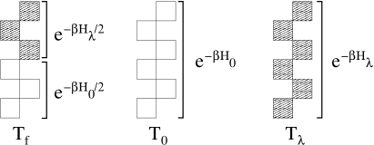
Figure 1: Transfer matrices for calculating $F(T)$. Each open [shaded] plaquette represents a local Boltzmann weight $\exp(-\epsilon h_{0}^{r,r+1})$ [$\exp(-\epsilon h_{\lambda}^{r,r+1})$], respectively, with $\epsilon$ being the Trotter parameter.

The spectra of these transfer matrices have a gap between the largest and the next-leading eigenvalue thus allowing it to perform the thermodynamic limit exactly Sirker and Klümper (2002a). For the fidelity density we find

$$f_{T}(\lambda)=-\frac{1}{N}\ln F=-\frac{1}{4}\ln\left(\frac{\Lambda_{f}}{\sqrt{\Lambda_{0}\Lambda_{\lambda}}}\right)$$ (7)

where $\Lambda_{f}$, $\Lambda_{0}$, and $\Lambda_{\lambda}$ are the largest eigenvalues of the transfer matrices $T_{f}$, $T_{0}$, and $T_{\lambda}$ defined in Fig. 1, respectively. Because $f_{T}(0)=\partial f_{T}/\partial\lambda|_{\lambda=0}=0$ we can calculate the fidelity susceptibility by $\chi_{f}(T)=2\lim_{\lambda\to 0}f_{T}(\lambda)/\lambda^{2}$, i.e., without having to resort to numerical derivatives. The transfer matrices can be efficiently extended in imaginary time direction - corresponding to a successive reduction in temperature - by using a density-matrix renormalization group algorithm applied to transfer matrices (TMRG). If we are mainly interested in $\chi_{f}$ then only small parameters $\lambda$ have to be considered, allowing it to renormalize all three transfer matrices with the same reduced density matrix. Apart from the two different Boltzmann weights necessary to form the three transfer matrices depicted in Fig. 1 the algorithm can therefore proceed in exactly the same way as the TMRG algorithm to calculate thermodynamic quantities. For technical details of the algorithm the reader is therefore referred to Refs. Bursill et al. (1996); Sirker and Klümper (2002a).

In the following, we want to study $\chi_{f}(T)$ for the $XXZ$ model defined by

$$H=J\sum_{r}\left\{S^{x}_{r}S^{x}_{r+1}+S^{y}_{r}S^{y}_{r+1}+\Delta S^{z}_{r}S^{z}_{r+1}\right\}$$ (8)

with respect to a change in anisotropy $\Delta$. Here $\boldsymbol{S}$ is a spin $S=1/2$ operator and $J$ the exchange constant which we set to $1$. We note that $\chi_{f}$ at zero temperature for finite chains has previously been studied in Venuti and Zanardi (2007); Chen et al. (2007). The model is gapless for $-1\leq\Delta\leq 1$ and gapped for $|\Delta|>1$. At $\Delta=0$ the model describes non-interacting spinless fermions and $\chi_{f}$ can be calculated exactly. The various diagrams can be combined into two contributions

$$\chi_{f}^{(1)} \!\!\!\!\!= \!\!\!\!\!\frac{1}{4\pi^{3}}\!\int_{-\pi}^{\pi}\!\!\!\!\!dk_{1}\,dk_{2}\,dk_{3}\frac{1-\text{e}^{-\beta x/2}}{x^{2}}y\bar{n}^{F}_{k_{1}}\bar{n}^{F}_{k_{2}}n^{F}_{k_{3}}n^{F}_{k_{1}+k_{2}-k_{3}}$$

$$\chi_{f}^{(2)} \!\!\!= \!\!\!\frac{1}{16\pi^{3}T^{2}}\left[\int_{-\pi}^{\pi}\!\!\!\!\!dk\,\cos k\,n^{F}_{k}\right]^{2}\int_{-\pi}^{\pi}\!\!\!\!\!dk\,\cos^{2}k\,n^{F}_{k}\,\bar{n}^{F}_{k}$$ (9)

with $x=\cos k_{1}+\cos k_{2}-\cos k_{3}-\cos(k_{1}+k_{2}-k_{3})$, $y=\cos^{2}(k_{1}-k_{3})-\cos(k_{1}-k_{3})\cos(k_{2}-k_{3})$, $n^{F}_{k}=1/[1+\exp(\beta\cos k)]$ and $\bar{n}^{F}_{k}=1-n^{F}_{k}$. The first contribution at low temperatures yields $\chi_{f}^{(1)}=0.19537(\pm 5)+\mathcal{O}(T^{2})$ whereas the second is given by $\chi_{f}^{(2)}=T/(6\pi)$. In the inset of Fig. 2 the exact solution for $\Delta=0$ is compared with the TMRG data obtained from $\chi_{f}=2f(\Delta+\delta\Delta)/(\delta\Delta)^{2}$ with $\delta\Delta=10^{-3}$.

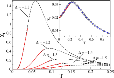
Figure 2: TMRG data (dashed) and fits (solid lines) for $\chi_{f}(T)$ in the ferrmomagnetic Ising regime. Inset: TMRG data for the free fermion case (circles) compared to the exact solution (dashed line) and the low-$T$ asymtotics (solid line).

The relative error without any extrapolation is less than $0.1\%$ for $T>0.1$ and less than $1\%$ for $T>0.04$.

In the gapped regime, $|\Delta|>1$, the fidelity susceptibility will show activated behavior. Following the arguments in Johnson and McCoy (1972) for the magnetic susceptibility we expect $\chi_{f}\sim T^{-3/2}\exp(-\gamma/T)$ with $\gamma=-\Delta-1$ being the spectral gap for $\Delta<-1$ and $\gamma$ being half the spectral gap for $\Delta>1$. Note that in the latter case the spectral gap is exponentially small for $\Delta\gtrsim 1$ making it difficult to detect numerically. As shown in Fig. 2 a fit of the data for $\Delta<-1$ is consistent with this scaling form with fitted $\gamma$ values close to the one theoretically expected.

In the gapless regime, $-1<\Delta\leq 1$, we know from the Bethe ansatz that $K=\pi/(\pi-\arccos\Delta)$ and $v=\pi\sqrt{1-\Delta^{2}}/(2\arccos\Delta)$. This allows us to check the universality of the contribution linear in $T$ in (6) by a direct comparison with the TMRG data (see Fig. 3) and to accurately extract $\chi_{f}(T=0)$.

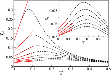
Figure 3: TMRG data (dashed) and low temperature fits (solid lines) for $\chi_{f}$ with the slope fixed by (6). The main figure (inset) shows data for $\Delta=-0.8,-0.7,\cdots,-0.1$ ($\Delta=0.1,0.2,\cdots,0.6$) from top to bottom, respectively.

This method fails, however, close to $\Delta=1$ where corrections due to Umklapp scattering start to become important (as will be discussed in more detail below) as well as very close to $\Delta=-1$ where the Luttinger model fails because the dispersion of the elementary excitations becomes quadratic. The fidelity susceptibility as a function of $\Delta$ for various temperatures as well as the extrapolated $T=0$ curve are shown in Fig. 4(a).

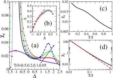
Figure 4: (a) The solid line depicts the extrapolated $T=0$ curve in the critical regime, the symbols the finite temperature curves as indicated on the plot. (b) The momentum cutoff $\Lambda$ as a function of $\Delta$ (symbols). The dashed line shows a fit for $\Delta\gtrsim-1$. (c) $\chi_{f}(T)$ for $\Delta=1$, and (d) for $\Delta=-1$ with the dashed line representing a low-$T$ fit as discussed in the text.

Comparing with the theoretical result (6) we can also extract the momentum cutoff $\Lambda$ (see Fig. 4(b)). There is a clear divergence of $\chi_{f}$ at the first order phase transition $\Delta=-1$. A fit of the extrapolated zero temperature curve shown in Fig. 4(a) gives $\chi_{f}(\Delta\gtrsim-1)\sim 0.017/(\Delta+1)^{1.26}$. This requires that the cutoff $\Lambda$ vanishes for $\Delta\to-1$ because otherwise we would find from (6) a divergence $\sim 1/(\Delta+1)^{2}$ as predicted in Yang (2007). Indeed, a fit of the extracted momentum cutoff as shown in Fig. 4(b) yields $\Lambda\sim 0.43(\Delta+1)^{0.65}$ and therefore $\chi_{f}(\Delta\gtrsim-1)\sim 0.013/(\Delta+1)^{1.35}$ which is consistent with the direct fit.

At the Kosterlitz-Thouless (KT) phase transition, $\Delta=1$, on the other hand, the behavior is different. Here the finite temperature data show that a maximum in $\chi_{f}$ at $\Delta>1$ exists which shifts to smaller $\Delta$ with decreasing temperature. The dependence of the cutoff $\Lambda$ near $\Delta=1$ seems to be consistent with $\Lambda\sim\Lambda_{1}+(1-\Delta)^{\alpha}$ with a constant $\Lambda_{1}$ and an exponent $\alpha$ both greater than zero. If this is indeed the case, we find from (6) that $\chi_{f}(\Delta\lesssim 1)\sim\Lambda_{1}/[16\pi^{2}(1-\Delta)]$.

Finally, we want to discuss the temperature dependence of $\chi_{f}$ right at the phase transitions. For $\Delta=-1$, shown in Fig. 4(d), we find a divergence $\chi_{f}\approx 0.002(\pm 1)T^{-2.5(\pm 1)}$ where the error is determined by a variation of the fit interval. As argued above, we also expect $\chi_{f}(T)$ to diverge for $T\to 0$ and $\Delta=1$. The numerical data, shown in Fig. 4(c), however, do not easily allow to extract the low temperature behavior. If we assume that $\lim_{\Delta\to 1}\Lambda=\Lambda_{1}>0$ then we can calculate the temperature dependence analytically as follows. At the isotropic point, Umklapp scattering is marginally irrelevant and the Luttinger parameter has to be replaced by a running coupling constant $K\to 1+g_{\parallel}(l)/2$ where $l=\ln T_{0}/T$ with a scale $T_{0}$ of order $J$ and $g_{\parallel}(l)=(2K^{*}-2)/\tanh[(2K^{*}-2)l+{\rm atanh}((2K^{*}-2)/g_{\parallel}^{0})]$ Giamarchi (2004). For $T=T_{0}$ we have $l=0$ and $g_{\parallel}(0)=g_{\parallel}^{0}$ while for $T\to 0$ it follows that $l\to\infty$ and $K=1+g_{\parallel}/2\to K^{*}$ where $K^{*}$ is the fix point value. For $l$ large we can neglect the part $\propto g_{\parallel}^{0}$. We therefore obtain

$$\chi_{f}(\Delta=1,T) = \lim_{\Delta\to 1}\frac{\Lambda_{1}}{32(1+g_{\parallel}/2)^{2}}\left(\frac{\partial g_{\parallel}}{\partial\Delta}\right)^{2}$$ (10)

$$\stackrel{{\scriptstyle T\ll T_{0}}}{{\to}} \frac{2\Lambda_{1}}{9\pi^{4}}\ln^{2}(T_{0}/T)\;.$$

While this prediction resolves some confusion about the behavior of $\chi_{f}$ at a KT transition Venuti and Zanardi (2007); You et al. (2007); Chen et al. (2007); Yang (2007) it cannot be reliably tested by comparing with the TMRG data. While the term in (10) should dominate at very low temperatures, subleading corrections might be of equal importance in the temperature range accessible numerically.

To summarize, we have shown that the fidelity susceptibility for the Luttinger model has a universal term linear in temperature or inverse length. Apart from being relevant for quantum phase transitions we believe that this result is also important to analyze sudden quantum quenches. Furthermore, we have introduced a numerical method to calculate the finite temperature fidelity in the thermodynamic limit for any 1D quantum system with short range interactions. Finally, based on a RG treatment, we have predicted a $\ln^{2}T$ divergence of $\chi_{f}$ at the KT transition in the $XXZ$ model.