Deep Near-Infrared Imaging of the $\rho$ Oph Cloud Core:
Clues to the Origin of the Lowest-Mass Brown Dwarfs

Abstract

A search for young substellar objects in the $\rho$ Oph cloud core region has been made with the aid of multiband profile-fitting point-source photometry of the deep-integration Combined Calibration Scan images of the 2MASS extended mission in $J,\,H$ and $K_{s}$ bands, and Spitzer IRAC images at 3.6, 4.5, 5.8 and 8.0 $\mu$m. The field of view of the combined observations was $1^{\circ}\times 9.3^{\prime}$, and the 5 $\sigma$ limiting magnitude at $J$ was 20.5. Comparison of the observed SEDs with the predictions of the COND and DUSTY models, for an assumed age of 1 Myr, supports the identification of many of the sources with brown dwarfs, and enables the estimation of effective temperature, $T_{\rm eff}$. The cluster members are then readily distinguishable from background stars by their locations on a plot of flux density versus $T_{\rm eff}$. The range of estimated $T_{\rm eff}$ values extends down to $\sim 750$ K which, based on the COND model, would suggest the presence of objects of sub-Jupiter mass. The results also suggest that the mass function for the $\rho$ Oph cloud resembles that of the $\sigma$ Orionis cluster based on a recent study, with both rising steadily towards lower masses. The other main result from our study is the apparent presence of a progressive blueward skew in the distribution of $J\!-\!H$ and $H\!-\!K_{s}$ colors, such that the blue end of the range becomes increasingly bluer with increasing magnitude. We suggest that this behavior might be understood in terms of the ‘ejected stellar embryo’ hypothesis, whereby some of the lowest-mass brown dwarfs could escape to locations close to the front edge of the cloud, and thereby be seen with less extinction.

1 Introduction

Although it is widely assumed that brown dwarfs represent the low-mass extension of normal star formation (Boss, 2001), many of the details are not clear. One theoretical problem is to explain the existence of objects much smaller than the typical Jeans mass of a parent cloud ($\sim 1\,M_{\odot}$), especially in light of reports of objects with masses $\stackrel{{\scriptstyle<}}{{{}_{\sim}}}3M_{J}$ (Zapatero Osorio et al., 2002; Marsh et al., 2010). In particular, a possible proto brown dwarf of mass $1\!-\!2\,M_{J}$ has been reported by Barrado et al. (2009), although this finding has been refuted by Luhman & Mamajek (2010). In principle, such objects could be produced by the fragmentation of protostellar cores, which can collapse gravitationally provided there is sufficient radiative cooling to overcome gas pressure. The lower mass limit for this to occur is believed to be $\sim 1$ $M_{J}$, irrespective of the details of the fragmentation process (Whitworth & Stamatellos, 2008). Disks may play a significant role, either by gravitational fragmentation of single disks (Stamatellos & Whitworth, 2009a, b), or by encounters between disks (Shen & Wadsley, 2006). One potential difficulty with any of these models is that even if low mass objects are produced initially, subsequent accretion from the infalling cloud will increase the final mass of the object. This led Reipurth & Clarke (2001) to propose the ‘ejected stellar embryo’ model whereby the lowest-mass members of a multiple system are ejected due to dynamical instability before they can accrete sufficient material to begin hydrogen burning. Hydrodynamic simulations of small stellar clusters suggest that dynamical interactions play a key role in the formation of not only brown dwarfs, but stars in general (Clarke et al., 2004).

Observational estimates of the mass function provide important constraints on the above models. Such information can be gained using data from deep imaging of star formation regions at multiple wavelengths. Because brown dwarfs emit most of their radiation at wavelengths longward of 1 $\mu$m, the near infrared is particularly conducive to their detection (Lucas & Roche (2000), Lucas et al. (2005)). Such data can be compared with the spectral predictions of evolutionary models, enabling preliminary estimation of physical parameters such as mass and temperature. One model of interest is the dust-free “COND” model of Baraffe et al. (2003), which assumes that the dust grains have settled below the photosphere. It thus represents one extreme with respect to the absorption of photospheric radiation by dust, and is applicable to the “methane dwarfs” whose temperatures are $\stackrel{{\scriptstyle<}}{{{}_{\sim}}}1500$ K. At the other extreme is the “DUSTY” model (Chabrier et al., 2000), applicable to brown dwarfs at higher temperatures, in which the photospheric dust stays at its formation site in the atmosphere.

The $\rho$ Oph cloud core is a suitable site for the study of young brown dwarfs due to its youth, high rate of low-mass star formation and its relative proximity; recent estimates of its distance are $120\pm 5$ pc (Loinard et al., 2008) and $135\pm 8$ pc (Mamajek, 2008). We assume a distance of 124 pc, representing a weighted average of these estimates. The main cloud, L1688, is approximately $1\times 2$ pc in extent and contains a substantial number ($\sim 100$) of low-mass stars (Wilking et al., 2005) whose estimated age is $\sim 1$ Myr (Luhman & Rieke, 1999; Prato et al., 2003; Wilking et al., 2005). Here we describe the results of deep imaging of a dense portion of this cloud at multiple wavelengths in the near-infrared and explore the implications for brown dwarf formation models.

2 Observations and Data Processing

Our dataset includes the deep $J,\,H$ and $K_{s}$ images from the $\rho$ Oph calibration field of the Two Micron All-Sky Survey (2MASS) Extended Mission (Cutri et al., 2006) that were produced by combining 1582 observations made between 1997 and 2000 during the course of the main survey (Skrutskie et al., 2006). The result is a set of high dynamic range images in which the sensitivity has been increased by 3.5–4.5 magnitudes over that of the main survey. The 2MASS 90009 field, of size $1^{\circ}\times 9.3^{\prime}$, centered at $\alpha=16^{\rm h}27^{\rm m}15.6^{\rm s}$, $\delta=-24^{\circ}41^{\prime}23^{\prime\prime}$ (J2000), covers part of the $\rho$ Oph cloud core, and has limiting magnitudes (at the 5 $\sigma$ level) of 20.5, 20.0, and 19.0 at $J,\,H$ and $K_{s}$, respectively. Some additional information on the 2MASS Calibration Fields, and on this field in particular, is given by Plavchan et al. (2008a, b).

We supplement these images with archival data at 3.6, 4.5, 5.8, and 8.0 $\mu$m from IRAC (Fazio et al., 2004) on the Spitzer Space Telescope (Werner et al., 2004), based on observations made in 2004 Apr 27–May 7 as part of the c2d legacy project (Evans et al., 2003). The archival BCD images were reprocessed to correct for artifacts (including saturation, column pulldown, muxbleed, “jailbar” effects, instrumental background and pixel-value outliers) and mosaicked using the Spitzer Science Center MOPEX software.

Figure 1 shows the relationship of the observed field to an extinction map of the cloud core. For comparison purposes, the field has been divided into “cloud” and “exterior” regions. The lower boundary of the “cloud” region was chosen to coincide with the $A_{V}=5$ mag contour of Cambrésy (1999), at $\delta=-24.8^{\circ}$. Our “exterior” region was chosen to extend southward from declination $-24.9^{\circ}$, wherein $A_{V}<3$ mag. The two regions are therefore defined as follows:

Cloud:	$16^{\rm h}26^{\rm m}55.0^{\rm s}<\alpha<16^{\rm h}27^{\rm m}35.8^{\rm s};\quad-24^{\circ}48^{\prime}00^{\prime\prime}<\delta<-24^{\circ}11^{\prime}50^{\prime\prime}$
Exterior:	$16^{\rm h}26^{\rm m}55.0^{\rm s}<\alpha<16^{\rm h}27^{\rm m}35.8^{\rm s};\quad-25^{\circ}11^{\prime}22^{\prime\prime}<\delta<-24^{\circ}54^{\prime}00^{\prime\prime}$

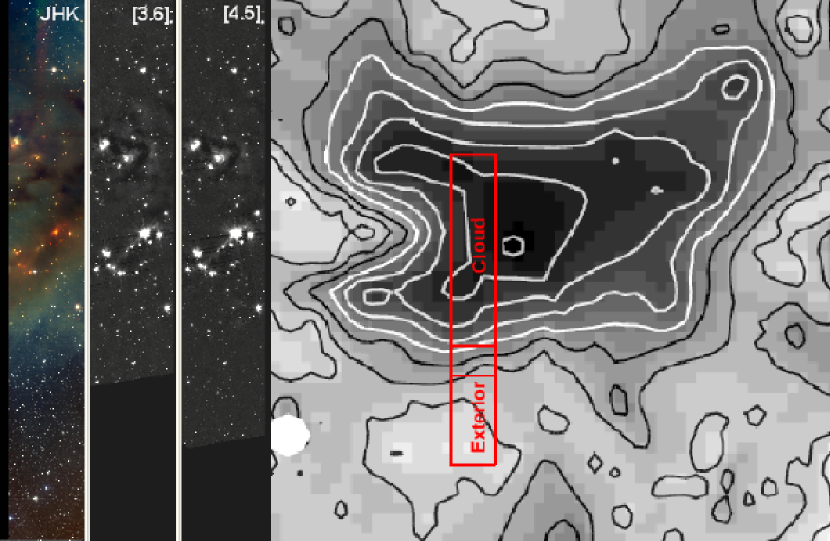
Figure 1: The observed region and its relationship to the $\rho$ Oph cloud core. The leftmost image is a composite of the 2MASS Deep Field $J,\,H$ and $K_{s}$ images (displayed in blue, green and red, respectively) with a field of view of $1^{\circ}\times 9.3^{\prime}$, centered on $\alpha=16^{\rm h}27^{\rm m}15.6^{\rm s}$, $\delta=-24^{\circ}41^{\prime}23^{\prime\prime}$ (J2000). To its right are the corresponding Spitzer IRAC images at 3.6 and 4.5 $\mu$m, respectively, obtained by reprocessing Spitzer archival data. The rightmost section of the figure represents an extinction map from Cambrésy (1999) upon which is superposed an outline of the field being studied (shown in far-left). Also indicated are the two subregions discussed in the text, namely “Cloud” and “Exterior.”

The image data from all seven bands were interpolated onto a common pixel-grid with a sampling interval of $0.5^{\prime\prime}$, spatially coincident with the 2MASS images. During this procedure, the Spitzer images were co-registered with the 2MASS images by matching the positions of bright stars, achieving a band-to-band registration accuracy of $\sim 0.2^{\prime\prime}$. These images were then processed using our MULTIPHOT profile-fitting source extraction procedure (Marsh & Cutri 2010, in preparation), which represents the multiband extension of the algorithm used for profile-fitting photometry in 2MASS. A key aspect is that the detection step and the source parameter estimation step are both done using the data at all bands simultaneously, thereby avoiding the ambiguities involved in bandmerging in crowded fields. The parameter estimation step represents a maximum likelihood solution to the source position ($\alpha,\delta$) and the set of multiband fluxes, taking into account the measurement noise and point spread function (PSF) at each wavelength. It provides a set of reduced chi squared values (for each band individually and an overall value) for testing the hypothesis that the data are consistent with a point source or a blend consisting of a small number of closely-spaced point sources. The noise model itself includes the effects of instrumental noise in the pixel values, PSF uncertainty, and uncertainty due to confusion error. The resulting derived error bars for flux and position are believed to represent a realistic assessment of the uncertainties in those quantities.

Care was taken to minimize any systematic effects in band-to-band flux calibration which would compromise the analysis of SEDs, including an assessment of the effects of confusion. Based on the relatively dilute field (on average, about 50 resolution elements per source) and the accurate band-to-band registration of the images discussed above, we are confident that the flux variations across bands (and, in particular, the 2MASS-Spitzer colors) are well-determined.

3 Results

Figure 2 shows color-magnitude diagrams ($H$ versus $J\!-\!H$ and $K_{s}$ versus $H\!-\!K_{s}$) for the $\rho$ Oph cloud region, and also for the region exterior to the cloud for comparison (see Figure 1). For both band/color combinations, the “cloud” and “exterior” plots are clearly quite different; the plots for the exterior region are consistent with relatively unobscured background stars, whereas the plots for the cloud region are consistent with stars at a wide range of visual obscurations.

For the $H$ versus $J\!-\!H$ plot of the cloud region, it is also evident that for most of the $H$ apparent magnitude range, the leftmost edge of the set of $J\!-\!H$ values is separated from the 1 Myr isochrone of the COND model by about 10 magnitudes of visual extinction, consistent with the star-forming cluster being embedded in the cloud at a depth corresponding to this opacity. However, for $H\stackrel{{\scriptstyle>}}{{{}_{\sim}}}18$ mag, this “minimum extinction” edge turns blueward, reaching zero extinction at $H\simeq 19.2$ mag. A similar blueward skew is apparent for the corresponding $K_{s}$ versus $H\!-\!K_{s}$ plot. We believe this effect is real since it is substantially larger than the observational error bars and is not evident for sources exterior to the cloud, as is apparent from Figure 2. It is also not an artifact of the profile-fitting source extraction process because the same blueward skew is evident when the extraction is repeated using aperture photometry via DAOPHOT (Stetson, 1987). The aperture photometry results are not plotted here, but can be accessed via Cutri et al. (2006).

Figure 2: Color-magnitude diagrams (left: $H$ versus $J\!-\!H$; right: $K_{s}$ versus $H\!-\!K_{s}$) for the $\rho$ Oph cloud (upper plots) and the region exterior to the cloud (lower plots), where the “cloud” and “exterior” regions are as defined in Figure 1. The plots include all detected point sources down to the 5 $\sigma$ level, where the sensitivity cutoffs are indicated by the straight solid lines. Typical error bars are indicated at the lower right on each plot, each at a vertical position corresponding to the applicable magnitude. The arrows represent the reddening vectors corresponding to 10 magnitudes of visual extinction. Also shown for each of the “cloud” plots is the 1 Myr isochrone from the COND model (Baraffe et al., 2003) for the mass values indicated (in units of solar masses), assuming 124 pc for the cloud distance.

If the extracted sources were all members of the star-forming cluster in the $\rho$ Oph cloud at 124 pc, then the faintest sources would correspond to low-mass brown dwarfs according to the COND model. It is likely, however, that many of the sources are external to the cloud and represent other types of object along the line of sight. Possibilities for the latter are more distant background stars, foreground T dwarfs, and extragalactic objects such as AGN. The first of those possibilities is suggested by previous measurements of the $K$-band luminosity function of the cloud core region, which is dominated by background stars for $K>15$ (Luhman & Rieke, 1999). Such objects would be most visible near the less-extincted edges of the cloud. Could they then account for the blueward skew seen in the color-magnitude diagrams of Figure 2? The answer is no, because any low-extinction window in the field would admit background stars over a wide range of magnitudes, and no blueward-turning edge would result.

In order to separate brown dwarfs from background stars we exploit the fact that these two classes of object are characterized by different color temperatures. Accordingly, we have fitted a temperature to each of the extracted sources from our multiband photometry. The technique, described in the next section, does not presume cluster membership a priori.

4 Temperature Estimation

We have estimated the effective temperature, $T_{\rm eff}$, of each extracted source based on a least squares fit of model spectra to the observed SEDs. The following suite of models was considered:

• COND (Baraffe et al., 2003) for an assumed age of 1 Myr.

• DUSTY (Chabrier et al., 2000) for the same assumed age.

• NextGen (Hauschildt et al., 1999) for stars of solar gravity and solar metallicity.

We have restricted these fits to five of our seven wavebands, namely $J,\,H,\,K_{s},\,[3.6]$ and $[4.5]$ because of their close wavelength correspondence with published COND and DUSTY model results at the $J,\,H,\,K,\,L^{\prime}$ and $M$ bands. This restriction does not negatively impact the temperature estimates since the sensitivity of IRAC at 5.8 and 8 $\mu$m is significantly less than for the shorter-wavelength bands. In addition, the photospheric fluxes at 5.8 and 8 $\mu$m are, in some cases, significantly contaminated by dust emission from circumstellar disks (Scholz et al., 2007).

For each hypothesized model, the procedure consisted of minimizing a function $\phi(T_{\rm eff},\alpha,A_{V})$ with respect to $T_{\rm eff}$, a flux scaling factor, $\alpha$, and the visual absorption, $A_{V}$, based on a functional form given by:

$$\phi(T_{\rm eff},\alpha,A_{V})=\sum_{\lambda=1}^{5}\frac{1}{\sigma_{\lambda}^{2}}[f_{\lambda}^{\rm obs}-\alpha 10^{-0.4r_{\lambda}A_{V}}f_{\lambda}^{\rm mod}(T_{\rm eff})]^{2}-\beta A_{V}$$ (1)

where $f_{\lambda}^{\rm obs}$ and $f_{\lambda}^{\rm mod}(T_{\rm eff})$ represent the observed and model fluxes, respectively, at the wavelength band represented by index $\lambda$; $\sigma_{\lambda}$ represents flux uncertainty; $r_{\lambda}$ represents the absorption in band $\lambda$ relative to $A_{V}$, based on the reddening law from Allers et al. (2006). The quantity $\beta$ is a constant whose significance we now discuss.

The 2nd term on the right hand side of (1) is designed to compensate for spurious biases towards low $T_{\rm eff}$ values resulting from the potential presence of long-wavelength excesses due to circumstellar dust. It is necessitated by the increasing degeneracy which exists between $T_{\rm eff}$ and $A_{V}$ as the temperature increases and the Rayleigh-Jeans regime is approached. Because of this degeneracy, the SED of a high-temperature object with large extinction can be reproduced equally well by a model based on a low-temperature object seen though small extinction. For such an object, the presence of even a relatively small long-wavelength excess due to circumstellar dust can favor a spurious low-temperature solution. To compensate for this effect, we have imposed a penalty against low values of $A_{V}$, whose severity is controlled by the value of $\beta$. We have optimized the value of $\beta$ using published photometry for a large number of spectroscopically-confirmed brown dwarfs of a variety of ages, as discussed in Appendix 1; the optimal value was found to be 0.7. This optimization incorporated the results of our own spectroscopic observations of 7 of the objects in our $\rho$ Oph source extraction list (Marsh et al., 2010).

In evaluating $\phi$, the model fluxes were calculated by logarithmic interpolation of the tabulated model fluxes with respect to $T_{\rm eff}$ and wavelength. The wavelength interpolation was necessitated by the mismatch between the observational wavebands (the Spitzer 3.6 $\mu$m and 4.5 $\mu$m bands) and the $L^{\prime}$ and $M$ bands for which the model photometry was tabulated. Although the wavelength mismatches are relatively small, some errors in the interpolation are inevitable. To assess this, we took some individual high resolution spectra from the COND models and smoothed them with the 2MASS and Spitzer bandpasses and found that $K_{s}\!-\![4.5]$ was accurately reproduced (to within 0.1 mag or better) but that $K_{s}\!-\![3.6]$ was less so, particularly at the lowest temperatures. Nevertheless, given the other errors involved in the temperature estimation procedure, we have found that this interpolation error is a relatively minor contributor.

For a given model, $T_{\rm eff}$ was restricted to the nominal range of physical validity, corresponding to $T_{\rm eff}<2000$ K (COND), $1800<T_{\rm eff}<3000$ (DUSTY), or $T_{\rm eff}>2200$ K (NextGen). For each extracted source, the estimates of $T_{\rm eff}$, $\alpha$, and $A_{V}$ were then based on the model which gave the minimum value of $\phi$. Such estimates were made for all sources detected in at least 4 of the 5 bands. Solutions which gave a poor fit, as indicated by a large value of reduced chi squared ($\chi_{\nu}^{2}>20$), were excluded. A total of 1022 successful fits was thereby obtained for the “cloud” region, representing 97% of the extracted sources. In particular it was found that the predicted spectral peculiarities of low temperature brown dwarfs ($T_{\rm eff}\sim 1000$ K) were well fit by the observations. Figure 3 shows some sample model fits to the dereddened fluxes, with estimated $T_{\rm eff}$ values as indicated.

Figure 3: Sample spectral fits, representing the results for two of the hotter objects (#34 and #2974) plus the 11 objects with the lowest estimated $T_{\rm eff}$. The filled circles with error bars represent the dereddened fluxes estimated from the observations, and the solid lines represent the best-fit model spectra. The latter were derived from the NextGen model for object #34, the DUSTY model for object #2974, and the COND model for the remaining 11 objects. Quantities in parentheses represent the formal uncertainties of maximum likelihood estimation of $T_{\rm eff}$ [K]. Note, however, that they do not take into account the effects of model error (see Appendix). The estimated $A_{V}$ values were (in order of decreasing $T_{\rm eff}$): 10.1, 20.2, 8.4, 1.5, 6.9, 9.2, 9.9, 7.2, 8.5, 11.3, 6.0, 7.3, and 1.1 mag. The corresponding values of reduced chi squared were: 1.1, 1.5, 1.3, 1.5, 1.4, 1.1, 1.2, 0.9, 19.7, 1.7, 2.4, 2.9, and 2.1.

The temperature fitting procedure was repeated for the “exterior” region. This region was not covered by the 3.6 $\mu$m observations and was incomplete at 4.5 $\mu$m, as can be seen from Figure 1. Nevertheless, temperature fitting was still possible with relatively little loss of accuracy. A total of 684 successful fits was thereby obtained, representing 100% of the extracted sources. This is comparable to the number of fits obtained for the “cloud” region even though the area of sky was substantially smaller. We verified that the lack of 3.5 $\mu$m data did not cause any systematic effects by repeating the “cloud” analysis without the 3.5 $\mu$m data.

Figure 4 shows plots of dereddened $K_{s}$ flux as a function of estimated temperature for the “cloud” and “exterior” regions. Also shown are the model curves for the COND and DUSTY models (age 1 Myr) and main sequence stars for an assumed distance of 124 pc.

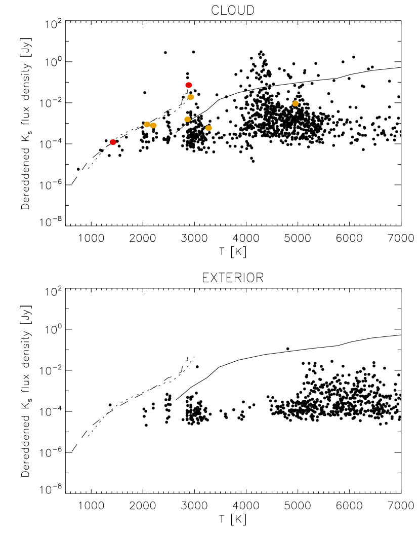
Figure 4: Dereddened $K_{s}$-band flux as a function of estimated temperature, for the $\rho$ Oph cloud (upper) and the cloud-exterior region (lower). The red symbols represent the results for the two spectroscopically-confirmed brown dwarfs in this region (objects #60 and #4450 in Table 1), the yellow symbols represent the six objects observed by Marsh et al. (2010) in addition to #4450, and the black symbols represent all other sources. Also shown are the model curves for the 1 Myr COND (dashed) and DUSTY (dotted) models, and main sequence stars (solid) for an assumed distance of 124 pc.

5 Cluster membership

Comparison of the two plots in Figure 4 shows that the number of points which fall on or close to the COND/DUSTY model curves is much greater on the “cloud” plot than on the “exterior” plot, consistent with the presence of brown dwarfs in the cloud core region. It is also apparent that the majority of points in the “exterior” plot correspond to $T_{\rm eff}\stackrel{{\scriptstyle>}}{{{}_{\sim}}}2800$ K and are below the main sequence line for a distance of 124 pc. They are therefore consistent with normal stars at distances larger than 124 pc. The same population is evident in the “cloud” plot, and hence the points which fall below the main sequence line on that plot can confidently be identified as background stars. They number 882 and 666 in the “cloud” and “exterior” regions, respectively. After exclusion of those objects we are left with $N_{\rm cloud}=139$ cluster member candidates in the “cloud” region and $N_{\rm ext}=18$ in the “exterior” region. This set of candidates may still, however, contain non-cluster contaminants. Possibilities include:

• Foreground L and T dwarfs.

• Extragalactic objects such as AGN.

• Main sequence background stars whose temperatures have been underestimated and which have therefore been incorrectly assigned to the brown dwarf regime in Figure 4.

The likelihood of foreground contamination by L and T dwarfs can be assessed from available number density statistics given that the volume of space in the cone capped by our “cloud” region is 54 pc³. Since the estimated space densities of L and T dwarfs in the solar neighborhood are $\sim 0.01$ pc^-3 in both cases (Burgasser (2007), Metchev et al. (2008)), the corresponding expectation numbers within this region are $\sim 0.5$ for both object types. This is consistent with estimates of the $J<21$ magnitude-limited sky density of T dwarfs (Burgasser et al., 2004) which would suggest $\sim 0.5$-1.0 such objects in a region of this size. We therefore conclude that the number of low-$T_{\rm eff}$ foreground objects in the “cloud” region is relatively small.

We can obtain an upper limit to the number of extragalactic contaminants by assuming that all of the inferred cluster members in the “exterior” region are spurious. We can then predict the number of contaminating sources in the “cloud” region by scaling $N_{\rm ext}$ by the cloud:exterior background source count ratio, equal to 1.32 from the background source counts estimated above. On this basis, an upper limit for the number of non-cluster members included in $N_{\rm cloud}$ is 24, i.e. of our 139 cluster member candidates, the percentage of contaminating sources is between 0 and 17%.

A particularly interesting subset of the cluster member candidates in Figure 4 is the group of low-$T_{\rm eff}$ objects ($T_{\rm eff}<1800$ K), of which there are 11 in the “cloud” region—these are most likely low-mass brown dwarfs. By contrast, there is only 1 such object in the “exterior” region. The fact that the number of low-$T_{\rm eff}$ objects decreases so sharply when going from “cloud” to “exterior” supports their inferred cluster membership and argues strongly against their being extragalactic. Even the 1 low-$T_{\rm eff}$ object in the “exterior” region could be a foreground T dwarf based on the statistics quoted earlier. We therefore consider it unlikely that any of our low-mass brown dwarf candidates are extragalactic background sources. Presumably, the latter are shielded from the observed field by dust in the Galactic disk.

Is it possible that we have underestimated the background contamination due to the fact that background sources in the “cloud” region are much more heavily reddened than those in the “exterior” region? For example, do highly reddened AGN resemble brown dwarfs when viewed through the cloud? To test this, we have simulated the effect of viewing the “exterior” region through a dense dust cloud and have repeated our temperature fits using the artificially reddened data. We found that no value of applied $A_{V}$ could produce a significant population of brown dwarf false-positives, and therefore conclude that the majority of our brown dwarf candidates in the “cloud” region cannot be attributed to reddened background objects.

Having excluded the various classes of possible background objects on the above basis, we are left with a total of 165 candidate cluster members in the entire observed field, of which 92 are brown dwarf candidates. These 165 objects represent the sum of the number of objects in the cloud region (139), exterior region (18), and the gap between those two regions (8). The photometric results for the candidate cluster members are presented in Table 1, and the locations of all detected sources (observed in at least 4 bands) are plotted in Figure 5. In the latter, red and green symbols denote candidate cluster members and background stars, respectively. Also shown for comparison on the plot are our estimated contours of visual absorption, $A_{V}$; these were obtained by dividing the field of view into square cells of size $2^{\prime}\times 2^{\prime}$, finding the maximum value of $A_{V}$ for all stars falling into a given cell, and interpolating using a Gaussian convolution kernel.

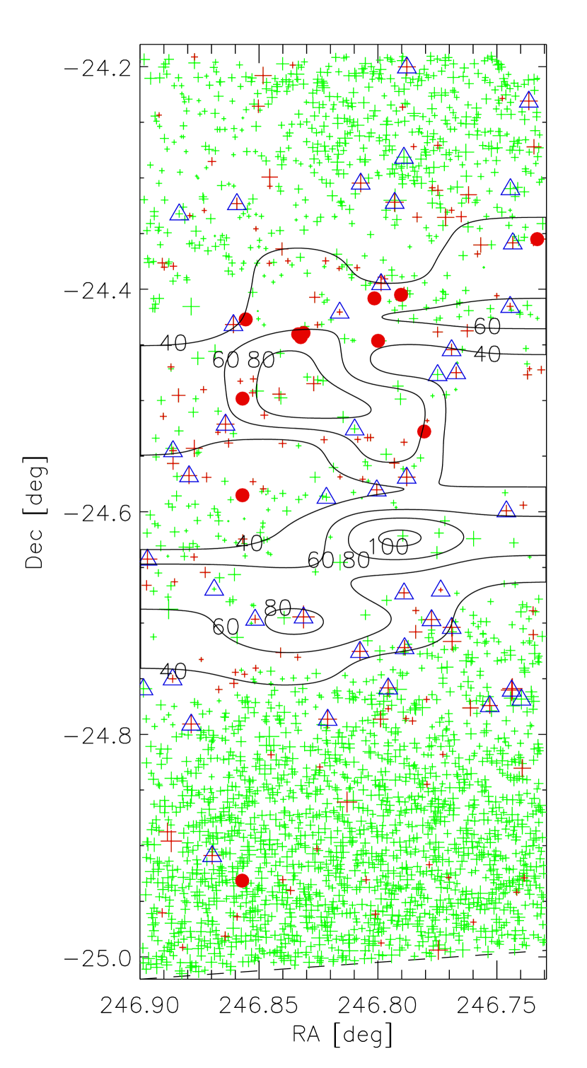
Figure 5: The spatial locations of detected sources in the $\rho$ Oph cloud. Red symbols denote candidate cluster members and green symbols denote inferred background objects. Filled circles represent candidate low-mass ($<5M_{J}$) brown dwarfs, and all other objects are indicated by crosses whose size increases with $K_{s}$ flux. Objects which coincide with known T Tauri stars/YSOs are enclosed by blue triangles. Also shown are contours of $A_{V}$, at levels of 40, 60, 80 & 100 mag. These go to deeper absorption levels than was possible with the optical star count technique used to generate the extinction contours shown in Figure 1, but are nevertheless consistent with the contours in that figure. The dashed line represents the limit of coverage at the IRAC bands. Note that the aspect ratio of this figure differs from that of Figure 1 in that the RA axis has been stretched to reduce the crowding of plotted symbols.

The fact that the background source density in Figure 5 is highest (by far) in the off-cloud region provides validation of our classification criterion for background stars. Likewise, the fact that the low-mass ($<5M_{J}$) brown dwarf candidates (filled red circles) are concentrated mostly in the cloud portion provides some confirmation of their identity as cluster members.

Color-magnitude plots for the candidate cluster members are shown in panels (a)-(c) of Figure 6. Also shown, for comparison, in the $K_{s}$ versus $K_{s}\!-\![3.6]$ plot of panel (c) are the locations of the inferred background stars. Since the $K_{s}\!-\![3.6]$ color is quite temperature-sensitive in the brown dwarf regime, the distributions of brown dwarfs and background stars are distinctly different on this plot. The fact that the blueward skew is still evident in the $JHK_{s}$ plots of (a) and (b) indicates that it is associated with objects in the $\rho$ Oph cloud, most likely brown dwarfs. The well-defined portion of the blueward skew has been delineated by the dashed lines on the plot; the objects which fall within this zone have been plotted as open circles in the $J\!-\!H$ versus $H\!-\!K_{s}$ color-color diagram of panel (d). The fact that the colors are positively correlated on this plot (i.e., blue $J\!-\!H$ corresponds to blue $H\!-\!K_{s}$) confirms that the blueward skew is not a random effect caused by increasing measurement errors. Does the blueward skew then indicate a deficiency in the models? This is unlikely, since the COND model is based on a dust-free photosphere and thus already produces relatively blue colors. A more likely explanation is that the faintest sources are seen with the least extinction. This could occur if the lowest-mass brown dwarfs are preferentially ejected from their formation sites and some are therefore seen closer to the front edge of the cloud along the line of sight. Such behavior would, in fact, be expected on the basis of the ‘ejected stellar embryo’ hypothesis, although models which involve ejection subsequent to the accretion phase would not be excluded.

An additional feature of the color-magnitude diagrams in Figure 6 is the dip in density of points around $H\sim 16$. Similar drops at comparable magnitudes have been found for other young clusters and star-forming regions (Muench et al., 2003; Lucas et al., 2005; Caballero et al., 2007). As discussed by Caballero et al. (2007), this phenomenon is yet to be understood, but it may be related to the deficit in M7 and M8 objects noted by Dobbie et al. (2002).

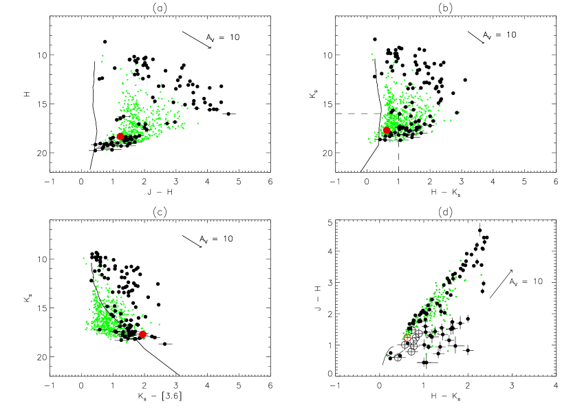
Figure 6: Color-magnitude and color-color diagrams for objects in the $\rho$ Oph cloud, subject to $S/N\geq 5$ at all bands on a given plot. Red symbols represent object #4450 (the spectroscopically confirmed low-mass brown dwarf), and black symbols represent all other cluster members. Green symbols represent inferred background stars. The open circles in the color-color diagram in (d) represent the cluster members within the zone delineated by the dashed lines in (b). Also shown for comparison are the predictions of the COND model for age 1 Myr (solid curves in (a)-(c)), and the loci of main sequence and giant stars (solid curves in (d)), from Bessell & Brett (1988).

6 The Mass Function

The temperature estimates can be used to infer a mass for each object in the “cloud” region, based on the assumed age. For those objects which were fit by the COND or DUSTY model, each temperature then corresponds to a unique model-based mass. For the hotter objects, which were best fit by NextGen, we used a mass-temperature relationship derived from observations by Greene & Meyer (1995) of pre-main sequence objects in the $\rho$ Oph cloud. Figure 7 shows a plot of $A_{V}$ versus mass, $M$, from which it can be seen that for $M\stackrel{{\scriptstyle<}}{{{}_{\sim}}}0.02\,M_{\odot}$, the minimum extinction for a given mass is positively correlated with the mass, reaching zero extinction for $M\sim 0.003\,M_{\odot}$ (3 Jupiter masses). No conclusion can be drawn for masses below about 0.001 $M_{\odot}$, however, since sources with significant extinction would be below the $J,H,K_{s}$ sensitivity limits for that mass range.

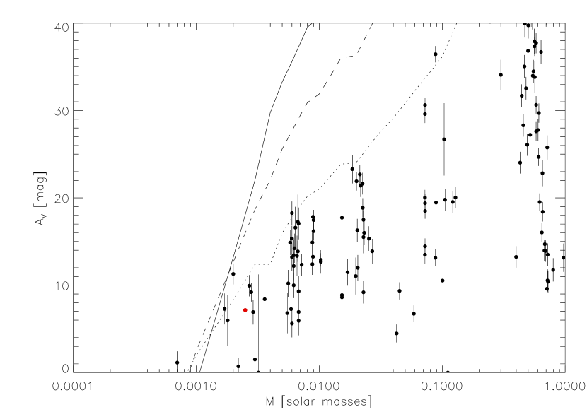
Figure 7: Estimated visual extinction as a function of estimated mass for objects in the $\rho$ Oph cloud. For reference, object #4450 is indicated in red. The 5 $\sigma$ sensitivity cutoffs for $J,\,H$ and $K_{s}$ are indicated by the dotted, dashed and solid lines, respectively.

The estimated mass function itself is plotted as a histogram in Figure 8. Sources of error in this plot include errors in mass estimation and misclassification as discussed in Section 5. The results given in the Appendix suggest that mass values have been estimated to an accuracy of a factor of $\sim 2-3$. The dashed line in the plot represents an estimate of the mass function based on the assumption that all inferred cluster members are genuine. We have corrected this result for likely contamination by foreground and background objects by making use of the results from the “exterior” region, assuming that all inferred cluster members in that region are spurious. Specifically, we constructed a separate mass function for the “exterior” region, scaled it by the cloud:exterior background source count ratio (1.32) estimated in Section 5, and subtracted the scaled histogram from the mass function of the “cloud” region. The result is indicated by the solid line in the figure.

Figure 8: The mass function for objects in the $\rho$ Oph cloud. The solid line (with error bars) represents our best estimate, based on an assumed age of 1 Myr in conjunction with the COND and DUSTY models. It has been corrected for the expected effects of contamination by foreground and background objects. The dashed line represents the estimate prior to applying the correction. Also shown for comparison are the estimated mass functions of $\rho$ Oph (Comeron et al., 1993) (open circles) and $\sigma$ Ori (Caballero et al., 2007) (filled circles) scaled on the vertical axis to match our results in the vicinity of 0.1 $M_{\odot}$.

The mass function, within the limits of uncertainty indicated in Figure 8, is consistent with the relatively flat distribution found previously in $\rho$ Oph for masses in excess of a few hundredths of a solar mass (Comeron et al., 1993), but departs significantly from this behavior for lower masses. Specifically, our results suggest an order of magnitude increase in the number of objects at $\sim 0.003\,M_{\odot}$ with respect to that at $\sim 0.1\,M_{\odot}$. The actual increase may be even larger than this, however; since some parts of the cloud have $A_{V}$ in excess of 100 magnitudes (see Figure 7), we may be missing some low-mass objects more deeply embedded in the cloud. The apparent flattening-out of the distribution below 0.002 $M_{\odot}$ is probably due to the sensitivity cutoff of the observations, as suggested by Figure 7. However, we cannot rule out the possibility of an actual cutoff in the mass distribution.

Our inferred mass function is consistent with that found for $\sigma$ Orionis (Caballero et al., 2007; Bihain et al., 2009) based on broad-band SED information using techniques somewhat similar to those used here. They similarly found an order-of-magnitude increase in the mass function between 0.1 and 0.006 $M_{\odot}$; the Caballero et al. (2007) results have been overplotted on our Figure 8 for comparison. In addition (Bihain et al., 2009) found a possible hint of a turnover at $\sim 0.004$ $M_{\odot}$, also reminiscent of Figure 8.

7 Discussion

We have cross checked our results against previous work by searching published lists of spectroscopically confirmed brown dwarfs in the $\rho$ Oph cloud core region, but could only find one such case within our field. This is GY 204, listed by Natta et al. (2002) as an M6 brown dwarf with a temperature of 2700 K and a mass of 40–80 $M_{J}$. It coincides with object #60 in Table 1 for which we had estimated $T_{\rm eff}=2888\pm 340$ K and a mass of $59^{+89}_{-35}\,M_{J}$, in agreement with the spectroscopic observation. We were able to match the majority of the brighter cluster member candidates to previously-known sources; for the 57 cluster-member candidates brighter than $K_{s}=14$, all but one corresponded to objects listed in the SIMBAD database. Of those 56, all were consistent with being young objects associated with the $\rho$ Oph cloud. This provides some additional confidence in the assigned cluster membership.

Our results suggest that the mass function for the $\rho$ Oph cloud core is similar to that of another young cluster, $\sigma$ Orionis (Bihain et al., 2009). A key feature is the increasing abundance with decreasing mass; this may be a consequence of the fragmentation of larger star-forming cores.

The distributions of $J\!-\!H$ and $H\!-\!K_{s}$ colors for the lowest-mass objects ($\stackrel{{\scriptstyle<}}{{{}_{\sim}}}0.005\,M_{\odot}$) show a progressive blueward skew with decreasing flux, which we interpret in terms of decreasing dust extinction with decreasing mass. That is not to say that all low-mass objects have low extinction, but rather that some of them make it out to the front edge of the cloud where we see them unextincted. Such behavior might be expected based on models in which the lowest-mass members of the cluster have been dynamically ejected from a formation site deep in the cloud. It is consistent with the timescales involved; dynamical simulations suggest brown dwarf ejection velocities of the order of a few km s^-1 (Reipurth & Clarke, 2001), adequate to traverse the $\rho$ Oph main cloud, of size $\sim 1$–2 pc (Wilking et al., 2005), within the assumed 1 Myr age of the cloud.

The spatial distribution of our low-mass ($M<5M_{J}$) brown dwarf candidates is distinctly different from that of the higher-mass T Tauri stars and YSOs, as shown in Figure 5. One of the key differences is that, surprisingly, the low-mass candidates are less dispersed than the T Tauri stars, contrary to the expectations of the ejection model. Another key difference is that most of the low-mass candidates are concentrated in the northernmost of the two dust filaments in this field ($\delta\sim-24.5^{\circ}$) and are absent from the southern filement ($\delta\sim-24.7^{\circ}$), even though the latter contains a somewhat higher concentration of T Tauri stars. This contrasts with the findings of Luhman (2006), whose study of the Taurus star-forming region indicated no significant difference between the distributions of stars and brown dwarfs. The situation is, however, somewhat reminiscent of spatial segregation effects in Taurus found by Guieu et al. (2007), whereby brown dwarfs with disks are preferentially located in one particular filament; no such segregation was evident for the T Tauri stars. Since the presence of a disk suggests youth, the spatial segregation might be interpreted in terms of age differences between different aggregates of objects in the region. Similarly, in the case of $\rho$ Oph, the relatively compact aggregate of low-mass candidates in the northern filament in Figure 5 may have resulted from a star formation event more recent than for some or all of the T Tauri stars. Therefore, the spatial compactness of the low-mass aggregate does not necessarily argue against the ejection model.

Alves de Oliveira et al. (2010) have recently compared our photometry with their own data, obtained in 2006, for the subset of 7 sources observed spectroscopically by Marsh et al. (2010), and found discrepancies in 3 cases. In particular, they found #4450 to be 1.42 magnitudes fainter than our estimate of $K_{s}=17.71$. After further examination of our images, we find the source to be slightly extended, with FWHM $\sim 2^{\prime\prime}-3^{\prime\prime}$. Its estimated flux will therefore depend to some extent on the aperture or beamsize used. We have estimated its $K_{s}$-band aperture magnitude from the 2MASS Deep Field data using apertures of various radii, making appropriate corrections for truncation of the point-source response, and obtain $K_{s}=18.34\pm 0.15$ in a $1.5^{\prime\prime}$ aperture. We have compared this result with that obtained from the $K$-band “peak-up” image during the spectroscopic observations of Marsh et al. (2010), which yield $K=18.57\pm 0.15$ for a $1.5^{\prime\prime}$ aperture; the image was unfortunately too noisy for larger apertures. The two magnitudes are nevertheless consistent within the error bars, and therefore suggest the absence of any significant source variability over the intervening $\sim 10$-year time span. There remains a significant discrepancy with the value $K_{s}=19.14\pm 0.2$ estimated by Alves de Oliveira et al. (2010), but we suspect that the difference can be attributed to the smaller effective beamsize ($0.4^{\prime\prime}-0.8^{\prime\prime}$) in the latter observations, which could lead to flux underestimation for an extended source. Object #4450 is not unique in this regard—we have found a number of other cases in which our sources are slightly extended, and hypothesize that we may be seeing the effects of scattering from remnant infalling dust envelopes surrounding the brown dwarf candidates. It is not clear what, if any, effect such cases would have on our temperature estimates, but we note that our SED fit for #4450 yielded an effective temperature in complete agreement with the spectroscopic value from Marsh et al. (2010).

Our conclusions are based on fits to broad-band SEDs which are subject to the uncertainties that we have discussed. Verification must await spectroscopic observations in order to confirm the nature of individual objects and to better constrain their parameters. Nevertheless, SED fitting can play an important role in gathering statistics over wider areas of the sky, which is important to do because the mass function is known to vary from region to region—between different star-forming clouds (Evans & Lada, 1991) and even within the same cloud (Barsony et al., 1997). Such studies will be aided by upcoming surveys, particularly the Wide-Field Infrared Survey Explorer (WISE) in conjunction with shorter-wavelength data from the UKIRT Infrared Deep Sky Survey (UKIDSS) and the Visible and Infrared Survey Telescope for Astronomy (VISTA). Additional complementary data, consisting of optical and far-red photometry, will soon be available from the Pan-STARRS-1 and Sky-Mapper survey telescopes, and will cover a larger area of sky than UKIDSS and VISTA.

APPENDIX: Validation of model-fitting technique based on spectroscopically-confirmed brown dwarfs

We have evaluated the performance of our model-fitting procedure using photometric data for cases of spectroscopically-confirmed brown dwarfs and young stellar objects taken from the literature. Our selection criteria were:

• The object must have been spectroscopically confirmed.

• The published photometry must include at least four of $J,\,H,\,K_{s}$, [3.6] (or $L$), and [4.5] (or $M$).

Figure 9: Evaluation of our technique for temperature estimation using photometric data for cases of spectroscopically confirmed brown dwarfs and young stellar objects taken from the literature. The plots show the effective temperature estimated from our SED fits as a function of the spectroscopically-determined value, as follows: Top: no constraint on $A_{V}$; Middle: $A_{V}$ constrained with $\beta=0.7$ (see text); Bottom: the effect of artifically applying an additional 50 mag of visual extinction. Open circles represent young (1-10 Myr) brown dwarfs using data from Caballero et al. (2007), Luhman et al. (2005a, b, 2007), Martin et al. (2001), Riaz et al. (2006) and Zapatero Osorio et al. (2000); filled circles represent the 7 young objects in $\rho$ Oph observed by Marsh et al. (2010); crosses represent field brown dwarfs using data compiled by Patten et al. (2006); open triangles represent T Tau stars from Wilking et al. (2005) and Gatti et al. (2006).

Figure 10: Comparison of our estimated $A_{V}$ with previously published values. The symbol convention is the same as for Figure 9.

The selected data then consisted of 4- or 5-band photometric measurements of 84 field brown dwarfs (ages 0.2–10 Gyr), 25 young brown dwarfs (ages $\sim 1$–10 Myr), the 7 young objects in $\rho$ Oph observed by Marsh et al. (2010), and all 8 of the 56 cross-identified SIMBAD objects for which a spectral type was available. Our model fitting procedure was run on these data in a manner identical to that used in Section 4, i.e., a maximum likelihood fit to three unknowns ($T_{\rm eff}$, $\alpha$, $A_{V}$) using the same assumed age (1 Myr) for the COND and DUSTY models. In each case, the SED-estimated temperatures were compared with the published spectroscopic values. In cases for which the latter had not been specified, it was inferred from the published spectral type using Figure 7 of Kirkpatrick (2005). The results are presented in Figure 9, the top panel of which shows the results obtained without the use of the $A_{V}$ constraint discussed in Section 4, i.e., $\beta=0$. The RMS difference between the estimated and spectroscopic values of $\log T_{\rm eff}$ for that case was 0.18, corresponding to a percentage error of 51% in the estimated value of $T_{\rm eff}$.

We have optimized $\beta$ by minimizing the RMS difference in $\log T_{\rm eff}$ as a function of $\beta$. In varying $\beta$ from 0 to 1.5, we find that the RMS difference goes through a well-defined minimum of 41% at $\beta=0.7$, and back up to 51% again; accordingly we select $\beta=0.7$ as the optimum value. The middle panel in Figure 9 shows the result. It is apparent that without the $A_{V}$ constraint, 6 of the 7 Marsh et al. (2010) objects would have been incorrectly assigned temperatures below 2000 K. A corresponding plot of our $A_{V}$ estimates versus the previously published values, where available, is shown in Figure 10.

In order to assess the sensitivity of our temperature estimation technique to the degree of extinction, we have artificially reddened the data by various amounts and repeated the estimation procedure. We find that the applied extinction produces very little perturbation in estimated temperature. As an example, the bottom panel of Figure 9 shows the effect of an applied $A_{V}$ of 50 mag.

For each estimated temperature, the models provide a corresponding mass which can be compared with the spectroscopically-estimated mass. For the young brown dwarfs, the RMS difference in log mass ($\log_{10}M$) between our estimates and previous spectroscopic determinations was 0.41, corresponding to an average error of a factor of $\sim 2-3$ in mass estimation.

Comparison between the uncertainties in $T_{\rm eff}$, $A_{V}$ in Table 1 and the scatter in these corresponding quantities in Figure 9 indicates that the true uncertainties are much larger than the formal errors of maximum likelihood estimation. The reason is that the latter represents the effect of random noise and does not take into account various sources of model error, which includes uncertainties in age, the reddening law, and the photospheric models themselves. The RMS residuals from the above evaluation therefore provide a more realistic assessment of the true uncertainties in the quantities estimated from the SED fits.

Table 1: Photometry and estimated effective temperatures, visual absorption, and masses of candidate cluster members in the $\rho$ Oph cloud core.

Obj#	RA	Dec	$J$	$H$	$K_{s}$	[3.6]	[4.5]	$T_{\rm eff}$	$A_{V}$	$M/M_{\odot}$
10	16 27 19.51	-24 41 40.2	9.401 (0.006)	8.654 (0.006)	8.404 (0.006)	8.569 (0.030)	8.184 (0.022)	5135 (1071)	2.3 (1.6)	1.849
14	16 27 15.13	-24 51 38.7	10.660 (0.006)	9.813 (0.006)	9.465 (0.006)	8.949 (0.027)	8.354 (0.022)	3033 (296)	3.5 (1.3)	0.112
17	16 27 9.10	-24 34 8.0	12.662 (0.006)	10.264 (0.006)	8.927 (0.006)	7.781 (0.046)	6.876 (0.026)	7319 (2872)	24.6 (1.4)	2.530
20	16 27 13.74	-24 18 16.7	12.296 (0.006)	10.258 (0.006)	9.241 (0.006)	8.548 (0.029)	7.632 (0.024)	5874 (1499)	18.1 (1.5)	1.994
21	16 27 32.86	-24 53 45.4	10.066 (0.006)	8.793 (0.006)	8.342 (0.006)	8.425 (0.036)	8.187 (0.023)	4426 (430)	4.7 (1.1)	0.687
22	16 27 17.08	-24 47 11.0	11.847 (0.006)	10.173 (0.006)	9.496 (0.006)	9.156 (0.026)	9.026 (0.023)	4451 (475)	9.6 (1.2)	0.711
23	16 27 5.17	-24 20 7.6	12.716 (0.006)	10.448 (0.006)	9.351 (0.006)	8.877 (0.029)	8.337 (0.023)	4382 (404)	16.0 (1.1)	0.646
24	16 27 27.38	-24 31 16.5	12.364 (0.006)	10.378 (0.006)	9.321 (0.006)	8.653 (0.030)	8.015 (0.023)	5348 (1258)	17.1 (1.5)	1.983
25	16 26 56.77	-24 13 51.4	12.390 (0.006)	10.388 (0.006)	9.323 (0.006)	8.250 (0.041)	7.582 (0.031)	8008 (8032)	20.6 (2.7)	2.814
27	16 27 30.85	-24 47 26.7	12.186 (0.006)	10.395 (0.006)	9.485 (0.006)	8.972 (0.027)	8.661 (0.023)	4643 (803)	13.1 (1.6)	0.971
28	16 27 10.32	-24 19 18.7	11.988 (0.055)	10.456 (0.025)	9.759 (0.021)	9.245 (0.065)	9.007 (0.053)	5127 (1180)	11.2 (1.7)	1.842
30	16 27 22.93	-24 17 57.3	13.314 (0.006)	10.695 (0.006)	9.397 (0.006)	8.771 (0.027)	8.187 (0.022)	4352 (346)	19.5 (1.0)	0.620
32	16 27 5.91	-24 59 37.8	11.526 (0.006)	10.436 (0.006)	10.068 (0.006)	$\cdots$	9.877 (0.022)	4804 (868)	5.2 (1.8)	1.297
34	16 27 4.52	-24 42 59.5	12.016 (0.006)	10.491 (0.006)	9.829 (0.006)	9.389 (0.028)	9.176 (0.022)	4812 (897)	10.1 (1.6)	1.314
35	16 27 1.63	-24 21 36.9	14.303 (0.006)	11.057 (0.006)	9.397 (0.006)	8.546 (0.027)	8.116 (0.023)	4256 (254)	27.2 (1.3)	0.519

Note. — The columns represent the object number, RA and Dec position (J2000), the magnitudes at the five bands indicated, the estimated effective temperature ($T_{\rm eff}$ [K]), visual absorption ($A_{V}$), and mass ($M$). Uncertainties are indicated in parentheses, with the exception of RA and Dec ($0.5^{\prime\prime}$ each) and $M$ (a factor of $\sim 2-3$). Table 1 is published in its entirety (165 objects) in the electronic edition of the Astrophysical Journal. A portion is shown here for guidance regarding its form and content.

References

- Allers et al. (2006) Allers, K. N., Kessler-Silacci, J. E., Cieza, L. A. & Jaffe, D. T. 2006, ApJ, 644, 364