Diameter Bounds for Planar Graphs

Abstract

The inverse degree of a graph is the sum of the reciprocals of the degrees of its vertices. We prove that in any connected planar graph, the diameter is at most $5/2$ times the inverse degree, and that this ratio is tight. To develop a crucial surgery method, we begin by proving the simpler related upper bounds $(4(|V|-1)-|E|)/3$ and $4|V|^{2}/3|E|$ on the diameter (for connected planar graphs), which are also tight.

1 Introduction

In this paper we examine the relation between “inverse degree” and diameter in connected planar simple graphs. The diameter $D(G)$ of a graph $G=(V,E)$ is the maximum distance between any pair of vertices, $D:=\max_{u,v\in V}dist(u,v),$ where as usual the distance between two vertices is the minimum number of edges on any $u$-$v$ path. The inverse degree $r(G)$ is a less well-studied quantity, and is defined equal to the sum of the inverses of the degrees, $r:=\sum_{v\in V}d^{-1}(v)$.

The history of inverse degree stems from the conjecture-generating program Graffiti [2]. Let $n$ denote $|V|$ and $m$ denote $|E|$. Graffiti posited that the mean distance $\tbinom{n}{2}^{-1}\sum_{\{u,v\}\subset V}dist(u,v)$ is always at most the inverse degree $r(G)$. This was disproved by Erdős, Pach & Spencer [1], who also proved the tight bound $D=O\bigl{(}\frac{\log n}{\log\log n}\cdot r\bigr{)}$ in the process. Subsequently, Mukwembi [3] studied the diameter for various kinds of graphs in terms of inverse degrees. Among other things he conjectured that for any planar graph $G$, $D(G)\leq\frac{9}{4}r(G)$.

We disprove Mukwembi’s conjecture and establish just how large $D/r$ can be:

Theorem 1.

For any planar graph $G$, $D(G)<\frac{5}{2}r(G)$. There is an infinite family of graphs with $D(G)=\frac{5}{2}r(G)-O(1)$.

The tight family we construct is very simple, but the bound $D(G)\leq\frac{5}{2}r(G)$ turns out to be quite challenging. A natural approach is to use the arithmetic-harmonic mean inequality to bound $r$ with the simpler quantity $r\geq\frac{n^{2}}{2m}$; to this end we prove the tight bound $D\leq\frac{4n^{2}}{3m}$ using a simple “surgery argument.”

However, the tight examples of graphs with $D=\frac{4n^{2}}{3m}-O(1)$ are non-regular (about $2/3$ of vertices have degree 5, and $1/3$ have degree 2) and so they are not tight for the ratio $D/r$ (since our use of the arithmetic-harmonic mean is tight only for regular graphs). Indeed, the bounds $D\leq\frac{4n^{2}}{3m}$ and $r\geq\frac{n^{2}}{2m}$ do not imply Theorem 1, but rather the weaker bound $D\leq\frac{8}{3}r$. To actually prove Theorem 1 (in Section 3) we carefully engineer a more intricate version of the surgery argument.

2 Initial Bounds from Surgery

In this section we focus on proving the less complex bound $D\leq\frac{4n^{2}}{3m}$, and on proving that the ratio $\frac{4}{3}$ is best possible, for connected planar graphs. We use the following sneaky attack on the problem:

Theorem 2.

For every connected planar graph, $D\leq\frac{4(n-1)-m}{3}$.

We give the proof later in this section, introducing our surgery approach along the way. It gives the desired corollary:

Corollary 3.

For every connected planar graph, $D\leq\frac{4n^{2}}{3m}$.

Proof.

We know $(2(n-1)-m)^{2}\geq 0$; rearranging yields $4(n-1)-m\leq 4\frac{(n-1)^{2}}{m}$, thus Theorem 2 yields $D(G)\leq\frac{4(n-1)-m}{3}\leq\frac{4(n-1)^{2}}{3m}$, which implies the corollary. ∎

We give some examples before proving Theorem 2. One example disproves Mukwembi’s conjecture, and the others demonstrate the tightness of the above theorems. For any even integer $n\geq 4$, let $L_{n}$ denote the graph with vertices $v^{i}_{j}$ for $i\in\{1,2\},1\leq j\leq n/2$, such that distinct nodes $v^{i}_{j},v^{i^{\prime}}_{j^{\prime}}$ are joined by an edge whenever $|j-j^{\prime}|\leq 1$; the left side of Figure 1 illustrates $L_{8}$. Its diameter is $D(L_{n})=n/2-1$, and its inverse degree is $r(L_{n})=\frac{n-4}{5}+\frac{4}{3}$. Hence $D=\frac{5}{2}r-O(1)$ for this family of graphs and the second half of Theorem 1 is proven.

Figure 1: These planar graphs are depicted as if they were drawn on a cylindrical tube, with the dashed edges hidden on the back. Left: the graph $L_{8}$. Right: the graph $T_{12}$.

Here is the tight example for Corollary 3: for any $n$ divisible by 3, take $L_{2n/3}$ and attach a path with $n/3$ additional nodes to $v^{1}_{1}$. The resulting graph has diameter $\frac{2n}{3}-1$ and $m=5\frac{n}{3}-4+\frac{n}{3}$ edges, so $\frac{4n^{2}}{3mD}$ tends to 1 as $n$ tends to infinity.

Finally, Theorem 2 is best possible, up to an additive constant, for all possible values of $m$ and $n$. Euler’s bound says that in planar graphs having $n\geq 3$, we have $m\leq 3n-6$; this maximum is achieved only for triangulations. For $n\geq 6$ divisible by 3, let $T_{n}$ be obtained from gluing a sequence of $\frac{n}{3}-1$ octahedra at opposite faces; we illustrate $T_{12}$ in the right side of Figure 1. To demonstrate tightness of Theorem 2 we start with the extremal values of $m$. For $m=n-1$ we have exact tightness: the path graph $P_{n}$ has $D(P_{n})=n-1=\frac{4(n-1)-m(P_{n})}{3}$. For $m=3n-6$ when 3 divides $n$, the graph $T_{n}$ has $D=\frac{n}{3}-1$ and $3n-6$ edges, which is tight for Theorem 2 up to an additive constant; other $n$ are similar. More generally, for any $n$ and any $n-1\leq m\leq 3n-6$, taking $T_{3\lceil(m+2-n)/6\rceil}$ and adding a path of $n-3\lceil(m+2-n)/6\rceil$ more vertices to one end gives an $n$-node, $m$-edge graph with $D=\frac{4(n-1)-m}{3}-O(1)$.

Now we give the proof of Theorem 2, which has some ingredients used later on: a surgery operation and decomposition into levels. In the proof, we will let $st$ be a diameter of $G$, e.g. $dist_{G}(s,t)=D(G)$. We let $V_{i}$, the $i$th level, denote all vertices at distance $i$ from $s$, hence $\biguplus_{i=0}^{D}V_{i}$ is a partition of $V$. We use the shorthand $V_{[i,j]}$ to mean $\uplus_{i\leq x\leq j}V_{x}$ and $V_{\geq i}$ is analogous. Additionally, $G[X]$ denotes an induced subgraph and we will extend the subscript notation on $V$ to mean induced subgraphs of $G$, for example $G_{\geq i}=G[V_{\geq i}]$.

Proof of Theorem 2.

Assume for the sake of contradiction that $G$ is a graph with $D(G)>\frac{4(n-1)-m}{3}$, assume that $n$ is minimal over all such graphs; we may clearly also assume $E$ is maximal in the sense that for any $e\not\in E$, either $G\cup\{e\}$ is non-planar or $D(G\cup\{e\})<D(G)$.

Our first step is to show that $G$ is 2-vertex-connected. Otherwise, pick an articulation vertex $v$, then we can decompose $G$ into graphs $G_{1},G_{2}$ with $V(G_{1})\cap V(G_{2})=\{v\},V(G_{1})\cup V(G_{1})=V(G),E(G_{1})\cup E(G_{2})=E(G)$, and $n(G_{1}),n(G_{2})<n(G)$ (a 1-sum). By our choice of $G$, both $G_{i}$’s satisfy the conclusion of Theorem 2. Moreover it is easy to see $m(G)=m(G_{1})+m(G_{2})$ and $D(G)\leq D(G_{1})+D(G_{2})$. Hence

$$D(G)\leq D(G_{1})+D(G_{2})\leq\tfrac{4(n(G_{1})-1)-m(G_{1})}{3}+\tfrac{4(n(G_{2})-1)-m(G_{2})}{3}=\tfrac{4(n(G)-1)-m(G)}{3},$$

contradicting the fact that $G$ was chosen to be a counterexample. Thus $G$ is indeed 2-vertex-connected.

We now consider the diameter $st$ and the level decomposition mentioned previously. Note that there are no edges between any pair of vertices in $V_{i}$ and $V_{j}$ if $|i-j|>1$. It is easy to see that if $|V_{i}|=1$ for some $0<i<D$ then $V_{i}$ is an articulation point, so we have (by 2-vertex-connectivity) that $|V_{i}|\geq 2$ for all $0<i<D$.

To begin, suppose $|V_{i}|\leq 2$ for all $i\neq 0$. Since each vertex can only connect to neighbours in $V_{i-1},V_{i},V_{i+1}$ the maximum degree is 5 (and 2 for $s$, 3 for $t$, 4 in $V_{1}$). Thus (assuming $n\geq 4$ which is easy to justify) we have $D=\lfloor\frac{n}{2}\rfloor$ and $m\leq\lfloor\frac{5n-7}{2}\rfloor$, whence it is easy to verify $D\leq(4(n-1)-m)/3$ as needed.

Hence, there exists a level of size $\geq 3$. We need one well-known fact and a technical claim.

Fact 4.

Let $G_{1},G_{2}$ be planar graphs with $V(G_{1})\cap V(G_{2})=\{u,v\}$ and $uv\in E(G_{1}),E(G_{2})$. Define their 2-sum $G$ by $V(G)=V(G_{1})\cup V(G_{2})$, $E(G)=E(G_{1})\cup E(G_{2})$. Then $G$ is planar.

Claim 5.

If $|V_{i}|=2$, $i<D$, then there is an edge joining the two vertices of $V_{i}$.

Proof.

Suppose otherwise. Let $V_{i}=\{u,v\}.$ We will show $uv$ can be added to $G$ without violating planarity, which will complete the proof, since $G$ was chosen edge-maximal (and adding $uv$ does not change $D$).

Since $G$ is 2-vertex-connected, $u$ is not an articulation vertex, so $G[\{v\}\cup V_{>i}]$ is connected, and similarly for $G[\{u\}\cup V_{>i}]$. Thus there is a path $P_{R}$ from $u$ to $v$ all of whose internal vertices lie in $V_{>i}$. Likewise there is a $u$-$v$ path $P_{L}$ all of whose internal vertices lie in $V_{<i}$ (e.g. concatenate shortest $u$-$s$ and $s$-$v$ paths).

Consider a drawing of $G$. The sub-drawing of $G_{\leq i}$ must have $u$, $v$ on the same face due to $P_{R}$, so $G_{\leq i}\cup\{uv\}$ is planar. Likewise $G_{\geq i}\cup\{uv\}$ is planar and using Fact 4, $G\cup\{uv\}$ is planar as needed. ∎

Recall there exists a level of size at least 3, let $L$ be chosen minimal with $|V_{L+1}|\geq 3$. Let $R$ be chosen maximal such that $R>L$, and all of the levels $V_{L+1},V_{L+2},\dotsc,V_{R-1}$ have size 3. Thus either $R=D+1$, or $R\leq D$ and $|V_{R}|<3$. We break into several similar cases now.

Case $L>0,R<D$. Thus $|V_{L}|=|V_{R}|=2$. Consider the graph $G^{\prime}$ obtained by “surgery” from $G$ by deleting all edges in $G_{[L,R]}$, deleting the isolated vertices $V_{[L+1,R-1]}$, then adding a clique on $V_{L}\cup V_{R}$. This is a planar graph by Fact 4 and Claim 5: it is obtained by two 2-sums from $G_{\leq L}$, $K_{4}$, and $G_{\geq R}$. We illustrate in Figure 2. Now $G^{\prime}$ is smaller than $G$; write $\Delta D=D(G)-D(G^{\prime}),\Delta m=m(G)-m(G^{\prime}),\Delta n=n(G)-n(G^{\prime})$. We have $\Delta n\geq 3\Delta D$ since all deleted levels had size at least 3. Moreover, since $G_{[L,R]}$ is a planar graph Euler’s bound gives that we deleted at most $3(\Delta n+4)-6$ edges and added 6 to the new clique, so $\Delta m\leq 3\Delta n$. Thus $\frac{4(\Delta n)-\Delta m}{3}\geq\frac{\Delta n}{3}\geq\Delta D$ and from this it is easy to verify that $G^{\prime}$ is a smaller counterexample to Theorem 2, contradicting our choice of $G$.

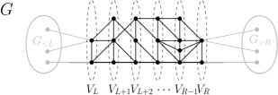
Figure 2: Depiction of how surgery changes a graph $G$ (left) into $G^{\prime}$ (right). Note the $V_{i},G_{i}$ labels are with respect to the original graph. Gray parts are unaltered.

Case $L>0,R\in\{D,D+1\}$. Let $X=V_{>L}\backslash\{t\}$. We delete all edges in $G_{\geq L}$, then the isolated vertices $X$, then we join the three vertices $V_{L}\cup\{t\}$ by a clique. Thus $\Delta m\leq 3(\Delta n+3)-6-3=3\Delta n$ and we proceed as before.

Case $L=0,R<D$ is the mirror image of the previous case (e.g. the clique is added to $V_{R}\cup\{s\}$).

Case $L=0,R\in\{D,D+1\}$. We have $n\geq 3D-1$ since all levels in $V_{[1,D-1]}$ have size at least 3. Using Euler’s bound, $4(n-1)-m\geq n+2>3D$ and $D<\frac{4(n-1)-m}{3}$ as needed. ∎

3 Proof that $r(G)\geq\frac{2}{5}D(G)$ for Planar Graphs

The general idea in the proof of Theorem 1 is similar to what we did in the previous section, but the devil is in the details, because the terms $1/d(v)$ change in quite complex ways when we perform surgery on the graph. For example, it is no longer possible to easily argue that the selected counterexample $G$ is 2-vertex-connected. Here is the sketch of how we prove $r(G)\geq\frac{2}{5}D(G)$.

• Define the fitness of a planar connected graph $G$ to be $\mathcal{F}(G):=\frac{2}{5}D(G)-r(G)$. So we want to show no graph has positive fitness.

• Let $n$ be minimal such that some $n$-vertex planar connected graph has positive fitness. Subject to this minimal $n$, take such a graph $G$ having maximal fitness. If another graph $G^{\prime}$ exists such that $|V(G^{\prime})|\leq|V(G)|$ and $\mathcal{F}(G^{\prime})\geq\mathcal{F}(G)$ and at least one of the these two inequalities is strict, this contradicts our choice of $G$. Therefore, the proof strategy uses several parts, and in each part we either find such a $G^{\prime}$, or impose additional structure on $G$.

• Let $st$ be any diameter of $G$. We show that except for $s$ and $t$, every vertex has degree at least 3, and that $s$ and $t$ have degree 2 or more.

• We lay out the graph $G$ in levels, as in the previous proof: level $V_{i}$ consists of all vertices at distance $i$ from $s$, hence $\uplus_{i=0}^{D}V_{i}$ is a partition of $V$.

• We arrive at a general “cornerstone” theorem (Theorem 20) showing that in many cases, a surgery like in Section 2 finds the desired $G^{\prime}$.

• We clean up some additional cases, and thereby prove that $G$ has at most 3 nodes per level, that no size-3 levels are adjacent, that for every size-2 level the contained nodes share an edge, and that the last level $V_{D}$ has size 1.

• We use a computation (Section 3.7) to prove that this structured graph has $\mathcal{F}(G)<0$, completing the proof.

3.1 Preliminaries

We reiterate the main tool in the proof.

Claim 6.

If $G^{\prime}$ is another graph obtained from $G$, with $n(G^{\prime})<n(G)$, such that $D(G^{\prime})\geq D(G)-\Delta D$, $r(G^{\prime})\leq r(G)-\Delta r$, and $\Delta r\geq\frac{2}{5}\Delta D$, then $G^{\prime}$ is smaller but at least as fit as $G$, contradicting our choice of $G$.

Since adding an edge decreases $r$ and increases fitness, we also have the following.

Claim 7 (Maximality).

If $uv\not\in E$ then either $G\cup\{uv\}$ is non-planar or $D(G\cup\{uv\})<D(G)$. In particular, when $u$ and $v$ are in the same levels or adjacent levels, since adding $uv$ would not change the diameter, we have that $G\cup\{uv\}$ is non-planar.

We will repeatedly make use of the arithmetic-harmonic mean in the following way.

Proposition 8.

For any set $S$ of vertices, $\sum_{v\in S}1/d(v)\geq|S|^{2}/(\sum_{v\in S}d(v))$.

Thus, the contribution to $r$ by any set is at least as big as what it would give “on average” by counting all endpoints incident on $S$. Later, we will count $\sum_{v\in S}d(v)$ as twice the number of edges of $G[S]$, plus the number of edges with exactly one endpoint in $S$.

Suppose that every level of $G$, except possibly the first and last ($V_{0}$ and $V_{D}$) have size 3. Then $n\geq 3(D-1)+2$ and the following proposition shows such graphs are not problematic.

Proposition 9.

If $n\geq 3(D-1)+2$, then $r(G)\geq\frac{2}{5}D$.

Proof.

The case that $|n|<3$ is easy to verify, so assume $|E|\leq 3n-6$. Proposition 8 applied to $S=V$ implies that $r\geq n^{2}/(6n-12)$, and by hypothesis $D\leq(n+1)/3$. Therefore it is enough to prove $n^{2}/(6n-12)\geq\frac{2}{5}(n+1)/3$, which is easy to verify by cross-multiplying and solving the resulting quadratic. ∎

3.2 Small-Degree Vertices and Articulation Points

Proposition 10.

$G$ does not have a degree-1 vertex.

Proof.

Let $v$ be a degree-1 vertex with neighbour $z$. We may assume $|V|\geq 3$ so $d(z)\geq 2$. How do $r$ and $D$ change if we get another graph $G^{\prime}$ by deleting $v$? Clearly $D$ decreases by at most 1; and $r(G^{\prime})=r(G)-\frac{1}{1}-\frac{1}{d(z)}+\frac{1}{d(z)-1}\leq r(G)-1/2$. In Claim 6 take $\Delta D=1$ and $\Delta r=1/2$, we are done. ∎

A repeated issue is that $r$ is not monotonic, i.e. sometimes we can decrease $r$ in a graph by adding extra vertices (e.g. consider the complete bipartite graphs, where $r(K_{2,10}<r(K_{1,10})$). The following proposition is a first attack against this issue and shows that adding extra blocks (2-vertex-connected components) cannot decrease $r$.

Proposition 11.

If $v$ is an articulation vertex of $G$, then $G\backslash v$ has exactly two connected components, one containing $s$ and one containing $t$.

Proof.

If the proposition is false, there is an articulation vertex $v$ such that a connected component $H$ of $G\backslash\{v\}$ contains neither $s$ nor $t$. Thus $G\backslash H$ contains $s$ and $t$, moreover $D(G\backslash H)=D(G)$ since any simple $s$-$t$ path goes through $v$ at most once and hence does not use any vertex of $H$.

We want to argue that $r(G\backslash H)\leq r(G)$, which will complete the proof using Claim 6 with $\Delta D=\Delta r=0$. It is enough to use very crude degree estimates. Let $|V(H)|=k$. Each vertex of $H$ has degree at most $k$ in $G$ since each $u\in V(H)$ can only have neighbours in $V(H)\cup\{v\}\backslash\{u\}$. Moreover, the difference between $r(G\backslash H)$ and $r(G)$ is due only to vertices in $\{v\}\cup V(H)$. Clearly $v$ has at least one neighbour not in $H$. Then

$$r(G)=r(G\backslash H)+\sum_{u\in H}\frac{1}{d_{G}(u)}+\frac{1}{d_{G}(v)}-\frac{1}{d_{G\backslash H}(v)}\geq r(G\backslash H)+\frac{k}{k}+0-1=r(G\backslash H),$$

as needed. ∎

Proposition 12.

Except possibly $s$ and $t$, $G$ does not have a degree-2 vertex.

Proof.

Let $v\not\in\{s,t\}$ be a degree-2 vertex, with neighbours $a,b$. If $a$ and $b$ are non-adjacent, we can remove $v$ and directly connect them, which decreases $r$ by 1/2 and decreases $D$ by at most 1, which yields a contradiction by Claim 6.

Therefore assume $a$ and $b$ are adjacent. If both $a$ and $b$ have degree 2 then $G=K_{3}$ and $\mathcal{F}(G)<0$, so we are done. If both $a$ and $b$ have degree at least 3, since $v\not\in\{s,t\}$, $G\backslash\{v\}$ is a connected planar graph with diameter at least as large as $G$ and $r(G^{\prime})\geq r(G)-1/2+1/6+1/6\geq r(G)$, so we are done by using Claim 6 with $\Delta D=\Delta r=0$.

The final case is that $a$ has degree 2 (w.l.o.g.) and $b$ has degree at least 3. Then $b$ is an articulation vertex, implying by Proposition 11 that $a\in\{s,t\}$, say w.l.o.g. $a=s$, and $t\not\in\{v,a,b\}$. But this contradicts edge-maximality in the following way: let $by$ for $y\not\in\{a,v\}$ be an edge on a common face with $bv$ (see Figure 3), then adding $vy$ to $G$ does not change the diameter. ∎

Figure 3: Dashed edges are added without violating planarity. (a) The edge $vy$ contradicting the edge-maximality. (b) The distance 2 neighbourhood of $s$ after $\omega$-$\mu$ surgery and the added edges.

3.3 Basic Surgery: Case Analysis and Bonuses

The central idea for surgery comes from the first case of Theorem 2’s proof.

Definition 13.

Given two levels $V_{L}$ and $V_{R}$, to apply surgery at $V_{L}$ and $V_{R}$ means to delete all nodes in $V_{[L+1,R-1]}$ (and their incident edges) and then to connect each $u\in V_{L}$ to each $v\in V_{R}$ (we “add a biclique”).

We say a level of size 2 is connected if its vertices share an edge, and that a level of size 1 is always connected. Assuming the levels are connected and of size at most 2, Definition 13 is indeed the same surgery as in Section 2. As before we get:

Proposition 14.

Suppose $|V_{L}|,|V_{R}|\leq 2$ are connected levels with $L<R$. Surgery at $V_{L}$ and $V_{R}$ yields a connected planar graph $G^{\prime}$ with $D(G^{\prime})=D(G)-(R-L-1)$.

We need a collection of types (cases) for our analysis. There are 7 types and $V_{L}$ may satisfy one or none of them (i.e. the cases are not exhaustive; nonetheless they form the core of our arguments). Analogous cases for $V_{R}$ are explained afterwards. Here are the 7 types for $V_{L}$:

• $L=0$, i.e. the level contains one end of the diameter $st$; for all other cases, $L>0$.

• $|V_{L}|=1$ and the node in $V_{L}$ has 1 neighbour in $V_{L-1}$

• $|V_{L}|=1$ and the node in $V_{L}$ has 2 neighbours in $V_{L-1}$

• $|V_{L}|=1$ and the node in $V_{L}$ has $\geq 2$ neighbours in $V_{L-1}$ and $\geq 2$ neighbours in $V_{L+1}$

• $|V_{L}|=2$, $V_{L}$ is connected, and each node of $V_{L}$ has 1 neighbour in $V_{L-1}$, in fact the same one

• $|V_{L}|=2$, $V_{L}$ is connected, and each node of $V_{L}$ has 2 neighbours in $V_{L-1}$

• $|V_{L}|=2$, $V_{L}$ is connected, and each node of $V_{L}$ has $\geq 2$ neighbours in $V_{L-1}$ and $\geq 2$ neighbours in $V_{L+1}$

The analogous cases for the right-hand side are the same with $L=0,L>0$ replaced by $R=D,R<D$, $V_{L}$ replaced by $V_{R}$, $V_{L-1}$ replaced by $V_{R+1}$, and $V_{L+1}$ replaced by $V_{R-1}$ (note the sign changes).

Fix $V_{L},V_{R}$ each of size $\leq 2$ with $L<R$, such that all levels in between have size at least 3. Our proof’s cornerstone, which we complete at the end of Section 3.5, is to show that when $L$ and $R$ are each of one of the 7 types, provided there are at least 4 nodes between $V_{L}$ and $V_{R}$, we can get a smaller $G^{\prime}$ which is at least as fit as $G$, by using surgery and some other “bonus” operations, contradicting our choice of $G$. After this cornerstone we deal with cases outside the 7 types.

First note that if both $L$ and $R$ are of type $\omega$, Proposition 9 already ensures $r(G)\geq\frac{2}{5}D(G)$. If $V_{L}$ is of type $\lambda$ and $V_{R}$ is of type $\xi$, we call the surgery type $\lambda$-$\xi$; we call $\omega$-$\omega$ the unneeded type of surgery since we don’t need to analyze it. It is essential to increase post-surgery fitness when possible. We now establish some values $bonus(\{\lambda,\xi\})$ (which are symmetric in $\lambda$ and $\xi$) such that, after a $\lambda$-$\xi$ surgery, we can increase the fitness by at least $bonus(\{\lambda,\xi\})$.

• We may take $bonus(\{\alpha,\beta\})=bonus(\{\alpha,\beta^{\prime}\})=\frac{1}{10}$ because this surgery results in a degree-2 vertex, which may be shortcutted to decrease $D$ by 1 and decrease $r$ by 1/2, giving a $\frac{1}{2}-\frac{2}{5}$ increase in fitness.

• Similarly we may take $bonus(\{\alpha,\alpha\})=\frac{2}{10}$.

• We may take $bonus(\{\omega,\beta\})=bonus(\{\omega,\beta^{\prime}\})=\frac{13}{30}$ as follows. Consider a $\omega$-$\beta$ (or $\beta^{\prime}$) surgery, so $V_{R}$ is a singleton $\{v\}$. After surgery $s$ has only one neighbour, $v$, and $v$ has degree at least 3. Then deleting $s$ decreases the diameter by 1 and decreases $r$ by at least $1-1/6$. Therefore there is a bonus of at least $1-1/6-2/5=\frac{13}{30}$.

• Similarly we can get $bonus(\{\omega,\alpha\})=13/30+1/10=8/15$ because (w.l.o.g. in a $\omega$-$\alpha$ surgery) the $\alpha$ vertex’s right neighbour has degree at least 3 in the original and post-operation graphs, using Proposition 12.

• Finally we can get $bonus(\{\omega,\mu\})=1/12$ as follows. Consider a (w.l.o.g.) $\mu$-$\omega$ surgery, where $V_{L}=\{u,v\}$ and the common neighbour of $u,v$ in $V_{L-1}$ is $w$. Post-surgery, the distance-2 neighbourhood of $s$ is as shown in Figure 3. Add a new vertex and connect it to $u,v,w,s$; it is not hard to argue this preserves planarity. Not counting the increased degree at $w$, we decreased $r$ by $\frac{1}{2}+\frac{2}{3}-\frac{1}{3}-\frac{3}{4}=\frac{1}{12}$ and preserved $D$. (Although this adds a vertex, the surgery theorems later on always delete at least 2 vertices, so overall the total number of vertices always decreases.)

3.4 First Analysis of Surgery

Now we give a lower bound on fitness increase due to surgery. It is convenient to assume when $V_{L}$ is in cases $\beta^{\prime},\nu^{\prime}$ that each node in $V_{L}$ has exactly two neighbours in $V_{L-1}$ — call the rest ghost neighbours. Why is this ok? Keep in mind we want to lower bound the fitness increase from surgery. Due to the “$\geq 2$ neighbours in $V_{L+1}$” condition in these cases, surgery does not increase the degree of nodes in $V_{L}$. Further, by the convexity of $d(v)\mapsto\frac{1}{d(v)}$, the actual $r$ increase including ghost neighbours will be no more than the “virtual $r$ increase” ignoring ghost neighbours made by our analysis.

Here are the details. Let $n_{L}$ denote $|V_{L}|$ and similarly for $n_{R}$. Let $o_{L}$ denote, for each node in $V_{L}$, the number of “outside” neighbours such nodes have in $V_{L-1}$; define $o_{R}$ similarly with $V_{R+1}$ in place of $V_{L-1}$. Thus $n_{L}$ and $o_{L}$ depend only on the type of $L$, and abusing notation, we write $n_{\omega}=n_{\alpha}=n_{\beta}=n_{\beta^{\prime}}=1,n_{\mu}=2,n_{\nu}=n_{\nu^{\prime}}=2$ and $o_{\omega}=0,o_{\alpha}=1,o_{\beta}=o_{\beta^{\prime}}=2,o_{\mu}=1,o_{\nu}=o_{\nu^{\prime}}=2$. Let $\overline{o}$ denote the number of neighbours each vertex of $V_{L}$ has in $V_{L}\cup V_{L-1}$, so $\overline{o}=o+(n-1)$. Let $w=R-L-1$ denote the number of levels in between, and recall that each of these $w$ levels has at least 3 nodes. Let $x$ denote the number of nodes in the deleted levels, hence we have $x\geq 3w$.

Before surgery, the sum of the degrees of the nodes in $V_{[L,R]}$ is at most $n_{L}o_{L}+2(3(n_{L}+x+n_{R})-6)+n_{R}o_{R}$ — the terms count edges from $V_{L-1}$ to $V_{L}$, in $G_{[L,R]}$, and from $V_{R}$ to $V_{R+1}$ respectively. We thereby use Proposition 8 to lower-bound the initial sum of the inverse degrees in $V_{[L,R]}$. Post-surgery, we know the degrees of the nodes in $V_{L}$ are $\overline{o}_{L}+n_{R}$ and similarly for $V_{R}$. Therefore, if $G^{\prime}$ indicates the result of applying surgery and bonus operations, we have $\mathcal{F}(G^{\prime})-\mathcal{F}(G)\geq\eqref{eq:mega}$ defined by

$$\frac{(n_{L}+x+n_{R})^{2}}{n_{L}o_{L}+2(3(n_{L}+x+n_{R})-6)+n_{R}o_{R}}-\frac{n_{L}}{\overline{o}_{L}+n_{R}}-\frac{n_{R}}{\overline{o}_{R}+n_{L}}+bonus(L,R)-\frac{2}{5}w. \ast$$ ()

It is easy to verify that $\eqref{eq:mega}>\frac{x}{6}-4-\frac{2}{5}w\geq\frac{x}{6}-\frac{2x}{15}-4$ so it is clearly positive for $x\geq 120$. In fact the following precise statement is true and gives what we want in almost all needed cases; we also need some $w=0$ cases for later even though they don’t make sense in the context provided above.

Claim 15.

Let $x,w$ be integers with $x\geq 3w,x\geq 2,w\geq 0$. Except for $(w,x)\in\{(1,3),(2,6)\}$, the value ($\ast$ ‣ 3.4) is positive for all types of $L,R$ (except the unneeded $L=R=\omega$).

Proof.

We use a publicly posted Sage worksheet [5] to verify the needed cases. (Note we’ve chosen things so that a $\lambda$-$\xi$ surgery has the same analysis as a $\xi$-$\lambda$ surgery, and such that the pairs $\{\beta,\beta^{\prime}\}$ and $\{\nu,\nu^{\prime}\}$ are analyzed in the same way. So our computation involves 14 surgery cases.)∎

More generally, the exact same proof gives the following generalization, which is needed later.

Theorem 16.

Let $V^{\prime}_{R}\subseteq V_{R}$, $L<R$, so that every $s$-$t$ path intersects $V^{\prime}_{R}$. Let $X$ be the nodes not connected to $s$ or $t$ in $G\backslash V_{L}\backslash V^{\prime}_{R}$ and let $x=|X|$. Let $V_{L}$ be any of the 7 types. Let $V^{\prime}_{R}$ be of one of the 7 types, modified so that “in $V_{R-1}$” is replaced by “in $X$” and “in $V_{R+1}$” is replaced by “in $V_{R+1}\backslash X$.” Assume that at least one of $L,R$ is not of type $\omega$. Let $w=R-L-1$. If we delete $X$ and connect $V_{L}$ to $V^{\prime}_{R}$ by a biclique, then perform bonus operations, we get a smaller graph at least as fit as $G$, provided $w\geq 0,x\geq 2$, $x\geq 3w$ and $(w,x)\not\in\{(1,3),(2,6)\}$.

3.5 Completing the Cornerstone: The Case $w=2,x=6$

If $w=2,x=6$ then $R=L+3$ and $|V_{L+1}|=|V_{L+2}|=3$, since all levels between $V_{L}$ and $V_{R}$ have size at least 3. We need:

Claim 17.

Let $V_{i}$ be a level of size 2, whose vertices are connected by an edge, and let $j=i+1$ or $j=i-1$, with $|V_{j}|=3$. Then the two vertices of $V_{i}$ do not have three common neighbours in $V_{j}$.

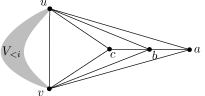
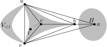
Figure 4: (a) If we delete $uvb$ the remainder will have at least 3 connected components. (b) One of these connected components, $H$, does not contain $s$ or $t$; we will delete it.

Proof.

The goal of the proof is similar to the result in Proposition 11: assume the opposite for the sake of contradiction, then show there is some part of the graph that can be deleted while decreasing $r$ and leaving $D$ unchanged. To do this, we need to establish some structure.

Let $V_{i}=\{u,v\}$. To simplify the notation we handle the case $j=i+1$ but the proof of the other case is identical. Since $G_{\leq i}$ is planar we can draw it with the edge $uv$ on the outer face. Likewise, draw $G_{\geq i}$ with $uv$ on the outer face. Each vertex of $V_{j}$ forms a triangle with $uv$ so for some labelling $V_{j}=\{a,b,c\}$, the drawing of $G_{\geq i}$ has triangle $uva$ containing vertex $b$ and triangle $uvb$ containing vertex $c$, as pictured in Figure 4.

We claim by maximality $ab$ is an edge of $G$: indeed, since $u$ has no neighbours other than $v,a,b,c$ in the drawing of $G_{\geq i}$, if $ab$ is not present we can add it in a planar way by going next to the path $aub$. Similarly $bc\in E(G)$.

Now note that $G\backslash\{u,b,v\}$ has at least 3 components: one containing $a$, one containing $c$, and one containing $V_{<i}$. One of the first two does not contain $t$. Assume the first (the second case is analogous): denote the component containing $a$ in $G\backslash\{u,b,v\}$ by $H$, so $H\not\ni t$ (see Figure 4). It’s not hard to see any shortest $s$-$t$ path avoids $H$, hence $D(G\backslash H)=D(G)$. Moreover we claim $r(G\backslash H)<r(G)$, contradicting our choice of $G$. To see this, let $k$ denote $|V(H)|$, note that each vertex in $H$ has degree at most $k+2$, and that we drop the degrees of $u,b,v$ by at most $k$, thus

$$r(G)-r(G\backslash H) \geq k\frac{1}{k+2}+\sum_{i\in\{u,b,v\}}\frac{1}{\deg_{G}(i)}-\frac{1}{\deg_{G\backslash H}(i)}$$

$$\geq\frac{k}{k+2}+\sum_{i\in\{u,b,v\}}\frac{1}{\deg_{G\backslash H}(i)+k}-\frac{1}{\deg_{G\backslash H}(i)}$$

$$\geq\frac{k}{k+2}+3(1/(k+3)-1/3)=\frac{k}{(k+2)(k+3)}>0$$

where in the second-to-last inequality we used the fact that $\deg_{G\backslash H}(i)\geq 3$ and $\frac{1}{\cdot}$ is convex. ∎

This allows us to bound the number of edges between a level $\{u,v\}$ with $uv\in E$ and an adjacent level of size 3: there are at most 5. It’s also obvious that between a singleton level and an adjacent level of size 3, there are at most 3 edges. Accordingly, let $z_{L}$ be 3 (resp. 5) when $n_{L}$ is 1 (resp. 2) and similarly define $z_{R}$. In the situation that there are exactly two levels, each of size-3, between $V_{L}$ and $V_{R}$, we can replace the quantity $\eqref{eq:mega}$ from the previous section by grouping the vertices in a different way; specifically we have $\mathcal{F}(G^{\prime})-\mathcal{F}(G)\geq\eqref{eq:mega2}$ with (✠ ‣ 3.5) defined by

$$\frac{n_{L}^{2}}{n_{L}\overline{o}_{L}+z_{L}}+\frac{x^{2}}{z_{L}+2(3x-6)+z_{R}}+\frac{n_{R}^{2}}{n_{R}\overline{o}_{R}+z_{R}}-\frac{n_{L}}{\overline{o}_{L}+n_{R}}-\frac{n_{R}}{\overline{o}_{R}+n_{L}}+bonus(L,R)-\frac{2}{5}w.$$ (✠)

Specifically, the first three terms lower-bound the contribution to $r(G)$ by vertices in $V_{L}$, in $V_{L+1}\cup V_{L+2}$, and $V_{L+3}=V_{R}$ respectively.

Claim 18.

The quantity (✠ ‣ 3.5) is positive when $w=2,x=6$ for all types of $L,R$ (except the unneeded type $L=R=\omega$).

Proof.

This calculation is also done via computer at [5].∎

Corollary 19.

Let $V_{L}$ and $V_{R}$ be levels of one of the 7 types (except the unneeded type $L=R=\omega$), with $R=L+3$ and $|V_{L+1}|=|V_{L+2}|=3$. Applying surgery at $V_{L}$ and $V_{R}$ gives a smaller which is smaller and more fit than $G$.

Together with Theorem 16 this gives the heart of our proof:

Theorem 20 (Cornerstone).

Let $V_{L},V_{R}$ be levels of size $\leq 2$, with all levels between them of size $\geq 3$. If $V_{L}$ and $V_{R}$ are each one of the $7$ types, and there are at least $4$ nodes between them, this contradicts our choice of $G$.

3.6 Sufficiency of the 7 Cases

The structure we want to establish in $G$ is that every level has size at most 3, and that two size-3 levels are never adjacent. We now show how to get from the cornerstone (Theorem 20) to this structure. We start with a general observation (which motivated our definition of the 7 cases).

Claim 21.

Suppose $V_{i}=\{u,v\}$ and $uv\in E$. Suppose $j=i\pm 1$, that $u$ has 1 or fewer neighbours in $V_{j}$, and that $v$ has at least one neighbour in $V_{j}$ which is not a neighbour of $u$. Then this violates maximality.

Proof.

Take $j=i+1$, the other case is analogous. Embed $G_{\geq i}$ with $uv$ on the outer face. First if $u$ has no neighbours in $V_{i+1}$ then note $u$ and a neighbour of $v$ are on the outer face, hence we can add an edge between them without violating planarity in $G_{\geq i}$ (and hence without violating planarity in $G$, by Fact 4). Second, suppose $u$ has exactly one neighbour $x$ in $V_{i+1}$; at least one endpoint emanating from $v$ adjacently to $vu$ is of the form $vy$ with $y\neq u,v,x$; then the path $uvy$ lies on a face and the edge $uy$ can be added without violating planarity. ∎

In the remainder of the section, we ensure all size-2 levels are connected, show that $V_{L}$ always is in one of the 7 cases, deal with $V_{R}$’s that fall outside the 7 cases, and then show the last level $V_{D}$ has size 1.

Claim 22.

Any level of size $2$ is connected, except possibly for the last level $V_{D}$.

Proof.

Let $V_{R}$ be minimal, $R<D$, such that $V_{R}=\{u,v\}$ is of size 2 and $uv$ is not an edge. If both $u$ and $v$ are connected to $t$ in $G_{\geq R}$ then using the proof method of Claim 5, $uv$ can be added without violating planarity, which contradicts maximality. Therefore assume only $u$ has a path to $t$ in $G_{\geq R}$. It now follows that $v$ is an isolated vertex in $G_{\geq R}$, or else Proposition 11 is violated because of the articulation point $v$.

Since $v$ has degree at least 3 (by Proposition 12) and these neighbours are only in $V_{R-1}$, it follows that $|V_{R-1}|\geq 3$. Let $L$ be maximal with $L<R$ such that $|V_{L}|\leq 2$. By our choice of $R$, we see $V_{L}$ is connected if it has size 2. Moreover, each vertex in $V_{L}$ has at least two neighbours in $V_{L+1}$, using $|V_{L+1}|\geq 3$ and Claim 21. So $V_{L}$ is of one of the 7 cases.

Now look at $u$. If $u$ has 2 or more neighbours in $V_{R-1}$, we can use surgery at $V_{L}$ and $u$ which is of type $\beta^{\prime}$ (Theorem 16: cutting out $R-L-1\geq 1$ levels of size 3, plus $v$). Otherwise, we can use surgery at $V_{L}$ and the unique neighbour of $u$ in $V_{R-1}$, which is an articulation vertex of type $\alpha$ (Theorem 16: cutting out $R-L-2\geq 0$ levels of size 3, plus $v$ and at least two nodes from $V_{R-1}$).∎

The following corollary follows from the previous proof and induction:

Corollary 23.

Every level $V_{L}$ such that $|V_{L}|\leq 2,|V_{L+1}|\geq 3$ falls in one of the 7 cases.

Proposition 24.

Let $V_{R}$, $R<D$, be such that $|V_{R}|\leq 2$, and either $|V_{R-1}|\geq 4$, or both $|V_{R-2}|,|V_{R-1}|\geq 3$. Then we can perform surgery to increase the fitness of $G$.

Proof.

Let $L<R$ be maximal with $|V_{L}|\leq 2$. Using Corollary 23 (along with Corollary 19 or Theorem 16) we may assume $V_{R}$ falls outside of the 7 types; using Claim 22 and Claim 21 this means that either $|V_{R}|=1$ and it has one neighbour in $V_{R-1}$ but $\geq 3$ neighbours in $V_{R+1}$, or $|V_{R}|=2$ and these vertices each have one neighbour (the same one) in $V_{R-1}$ and one vertex of $V_{R}$ has $\geq 3$ neighbours in $V_{R+1}$.

In either case, only one vertex in $V_{R-1}$, call it $v$, is adjacent to $V_{R}$. Since $v$ is an articulation vertex we can do surgery on $V_{L}$ and $v$ — we apply Theorem 16 to levels $L$ and $R^{\prime}=R-1$, on sets $V_{L}$ and $V^{\prime}_{R^{\prime}}=\{v\}$ (here $V^{\prime}_{R^{\prime}}$ is of type $\alpha$ if $|V_{R}|=1$ or $\beta$ if $|V_{R}|=2$). The set $X$ is $V_{[L+1,R-1]}\backslash\{v\}$, and $w=R^{\prime}-L-1$ so $x=|X|\geq 3w+2,w\geq 0$. This indeed satisfies the conditions of Theorem 16 so we are done. ∎

Proposition 25.

The size of the last level $V_{D}$ is 1.

Proof.

Suppose $|V_{D}|>1$ for the sake of contradiction. Let $V_{L}$ be the rightmost level of size at most 2, which we know is one of the 7 types by Corollary 23. Let $v\in V_{D}\backslash\{t\}$. If $L=D-1$ then it is not hard to see some face contains $v$ and a vertex from $V_{D-2}$; adding an edge between this pair does not decrease the diameter, so contradicts edge-maximality. Otherwise ($L<D-1$) apply surgery to $V_{L}$ and $t$: we cut out 1 or more levels of size at least 3, plus the vertices of $V_{D}\backslash\{t\}$. Thus $x\geq 3w+1,w\geq 1$ and Theorem 16 is satisfied. ∎

Combining the results just proven, we have the desired structure theorem: $G$ is a graph where the first and last level have size 1, all levels have size at most 3, every level of size 2 is connected, and no two levels of size 3 are adjacent.

3.7 Computation

We finish by showing that our hypothetical $G$ has $r\geq\frac{2}{5}D$.

Theorem 26.

Let $G$ be a graph where the first and last level have size 1, all levels have size at most 3, every level of size 2 is connected, and no two levels of size 3 are adjacent. Then $r(G)\geq\frac{2}{5}D+\frac{37}{60}$.

Proof.

The most important fact about the structure is that, given the sizes of levels $i-1,i,i+1$, we can determine (or upper bound, depending on how you look at it) the degrees of the nodes in level $i$, which we use to get a lower bound on the sum of the inverse degrees for that level.

Given any two adjacent levels, we may upper bound the edges they share by a biclique. Furthermore, if a level of size 2 and a level of size 3 are adjacent, by Claim 17 we can upper bound their shared edges as being one edge short of a biclique. Hence let $\mathcal{S}(i,j)=i\cdot j$ unless $\{i,j\}=\{2,3\}$ in which case $\mathcal{S}(i,j)=5$. Thus:

• $\sum_{v\in V_{0}}1/d(v)\geq 1/|V_{1}|$

• $\sum_{v\in V_{D}}1/d(v)\geq 1/|V_{D-1}|$

• For $0<i<D$ there are at most $\mathcal{E}:=\mathcal{S}(|V_{i-1}|,|V_{i}|)+2\tbinom{|V_{i}|}{2}+\mathcal{S}(|V_{i}|,|V_{i+1}|)$ endpoints incident on $V_{i}$; considering the degrees are integral and using convexity we see

  $$\sum_{v\in V_{i}}1/d(v)\geq\frac{\mathcal{E}\bmod|V_{i}|}{\lceil\mathcal{E}/|V_{i}|\rceil}+\frac{|V_{i}|-(\mathcal{E}\bmod|V_{i}|)}{\lfloor\mathcal{E}/|V_{i}|\rfloor}=:\mathcal{C}.$$

Since $\mathcal{C}$ is determined only by $|V_{i-1}|,|V_{i}|,|V_{i+1}|$, we write it as $\mathcal{C}(|V_{i-1}|,|V_{i}|,|V_{i+1}|)$. We therefore deduce for any sequence $(n_{0},n_{1},\dotsc,n_{D})$ of level sizes of a graph $G$ that

$$r(G)\geq\mathcal{R}(n_{0},n_{1},\dotsc,n_{D}):=1/n_{1}+1/n_{D-1}+\sum_{i=1}^{D-1}\mathcal{C}(|V_{i-1}|,|V_{i}|,|V_{i+1}|).$$

Finally, we want to determine which valid sequence minimizes $\mathcal{R}(n_{0},n_{1},\dotsc,n_{D})-\frac{2}{5}D$. Because $\mathcal{C}$ is a sum of local contributions, and because each level contributes 1 to the diameter, we can think of this last step as shortest path problem, as follows. Define a new digraph with vertex set

$$\{s,(1,1),(1,2),(1,3),(2,1),(2,2),(2,3),(3,1),(3,2),t\},$$

where the $(i,j)$-vertices represent a pair of adjacent levels, $s$ represents the start, and $t$ the end. The intuition: we insert an arc from $(i,j)$ to $(k,\ell)$ whenever $j=k$, representing three consecutive levels. The cost of such an edge should account for the $r$-contribution of the level corresponding to $j$, minus the contribution from lengthening the diameter.

Formally, we add an arc $(i,j)\rightarrow(j,k)$ for all $i,j,k$ (with no consecutive 3s) having cost $\mathcal{C}(i,j,k)-\frac{2}{5}$; we add an arc $s\rightarrow(1,i)$ for all $i$ having cost $1/i$; and we add an arc $(i,1)\to t$ for all $i$ having cost $1/i-\frac{2}{5}.$ Then it’s easy to see that for any sequence of $n_{i}$’s, $\mathcal{R}-\frac{2}{5}D$ is given by the cost of the $(D+1)$-edge path $s\to(n_{0},n_{1})\to(n_{1},n_{2})\to\dotsb(n_{D-1},n_{D})\to t$ in the new digraph. Executing a shortest-path algorithm such as Bellman-Ford (see the worksheet at [5]) establishes that the shortest path from $s$ to $t$ has cost $\frac{37}{60}$, hence $r\geq\mathcal{R}\geq\frac{2}{5}D+\frac{37}{60}$ for these graphs (and that there are no negative dicycles). ∎

In fact $r\geq\frac{2}{5}D+\frac{37}{60}$ holds for all graphs, is best possible, and the unique graph with $r=\frac{2}{5}D+\frac{37}{60}$ is $K_{5}^{-}$. To establish this precise result, small adjustments to our proofs are necessary, as well as exhaustive searching on all planar graphs with up to 9 vertices.

4 Conclusion

The main techniques underlying our diameter bounds for planar graphs were the surgery operation (which preserves planarity), and the fact that every planar graph has at most a linear number of edges. One might try the same approach on the family of graphs excluding any fixed $k$-clique minor, since such graphs have $O(nk\sqrt{\log k})$ edges (e.g., see [4]). A perpendicular avenue for future research would be to find a tight relation in connected planar graphs between the mean distance and the diameter.

References

- [1] P. Erdős, J. Pach and J. Spencer:On the mean distance between points of a graph, Congr. Numer. 64 (1988), 121 -124.
- [2] S. Fajtlowicz: On conjectures of graffiti II, Congr. Numer. 60 (1987), 189 -197.
- [3] S. Mukwembi: On diameter and inverse degree of a graph, Discrete Mathematics Volume 310, 4, 2010, 940–946.
- [4] A. Thomason: The Extremal Function for Complete Minors, Journal of Combinatorial Theory, Series B Volume 81, 2, 2001, 318–338.
- [5] http://sagenb.org/home/pub/2050