Magnetic Bose glass phases of coupled antiferromagnetic dimers with site dilution

Abstract

We numerically investigate the phase diagram of two-dimensional site-diluted coupled dimer systems in an external magnetic field. We show that this phase diagram is characterized by the presence of an extended Bose glass, not accessible to mean-field approximation, and stemming from the localization of two distinct species of bosonic quasiparticles appearing in the ground state. On the one hand, non-magnetic impurities doped into the dimer-singlet phase of a weakly coupled dimer system are known to free up local magnetic moments. The deviations of these local moments from full polarization along the field can be mapped onto a gas of bosonic quasiparticles, which undergo condensation in zero and very weak magnetic fields, corresponding to transverse long-range antiferromagnetic order. An increasing magnetic field lowers the density of such quasiparticles to a critical value at which a quantum phase transition occurs, corresponding to the quasiparticle localization on clusters of local magnets (dimers, trimers, etc.) and to the onset of a Bose glass. Strong finite-size quantum fluctuations hinder further depletion of quasiparticles from such clusters, and thus lead to the appearance of pseudo-plateaus in the magnetization curve of the system. On the other hand, site dilution hinders the field-induced Bose-Einstein condensation of triplet quasiparticles on the intact dimers, and it introduces instead a Bose glass of triplets. A thorough numerical investigation of the phase diagram for a planar system of coupled dimers shows that the two above-mentioned Bose glass phases are continuously connected, and they overlap in a finite region of parameter space, thus featuring a two-species Bose glass. The quantum phase transition from Bose glass to magnetically ordered phases in two dimensions is marked by novel universal exponents ($z\approx 2$, $\beta\approx 0.9$, $\nu\approx 1$). Hence we conclude that doped quantum antiferromagnets in a field represent an ideal setting for the study of fundamental dirty-boson physics.

I Introduction

Quantum phase transitions in spin-gapped antiferromagnets (AF) have been extensively studied both theoretically and experimentally. Several mechanisms exist which can drive these systems from a quantum disordered ground state with a finite spin gap to a gapless antiferromagnetic long-range ordered (AFLRO) state. Possible ways to close the spin gap are the modulation of the superexchange couplings by, e.g., mechanical deformation of the crystal under pressure Gotoetal06 , the application of a magnetic field Rice02 ; Zheludev05 ; Hondaetal ; Chaboussantetal97 ; Watsonetal01 ; Jaimeetal04 ; Sebastianetal05 ; Nikunietal00 ; Rueggetal03 ; Zapfetal06 ; Klanjseketal08 or the dilution of the system with non-magnetic impurities Uchiyamaetal99 ; Azumaetal97 ; Oosawaetal02 .

For definiteness we will discuss the case of spin-gapped systems with a singlet ground state, associated with the magnetic Hamiltonian of weakly coupled dimers. In these systems a finite singlet-triplet spin gap opens for sufficiently weak inter-dimer couplings. The application of a magnetic field to the system can close the gap at a critical value at which a quantum phase transition occurs, which is well described as a Bose-Einstein condensation (BEC) of $S=1$ triplets Nikunietal00 ; Giamarchietal08 ; Affleck91 ; GiamarchiT99 ; Matsumotoetal04 ; Kawashima04 ; MisguichO04 ; Wesseletal . The field has the combined effects of partially polarizing the dimers and inducing transverse AFLRO, which corresponds to a superfluid (SF) state of the field-induced triplets. Alternatively, doping weakly-coupled dimer systems with static non-magnetic impurities also has dramatic effects. Each dopant releases a spin-$1/2$ degree of freedom out of the singlet, and this $S=1/2$ moment gets exponentially localized around the site of the spin left unpaired Sorensen98 . Hereafter this localized $S=1/2$ degree of freedom will be denoted as local moment (LM). The overlap of the localized wave functions of two nearby LMs produces effective couplings that decay exponentially with the distance between the two impurities SigristF96 , and which alternate in sign depending on whether the LMs belong to the same sublattice or not, and consequently they are not frustrated. The resulting random network of LMs therefore develops AFLRO at $T=0$ for any finite doping concentration Laflorencieetal04 , and its low-energy excitations give rise to a phenomenon of order-by-disorder (OBD) ShenderK91 ; Wesseletal01 .

It is intriguing to investigate the nature of the ground state in a spin-gapped system when both factors perturb the gapped state, i.e., a magnetic field and non-magnetic impurities, are present. In this paper we focus on the interplay between site dilution and an applied magnetic field in a planar coupled dimer system. We provide a detailed picture of the rich phase diagram of the system, with particular emphasis on the emergence of an extended novel quantum-disordered phase with the nature of a Bose glass (BG), as introduced for three-dimensional systems in Refs. Nohadanietal05, ; Yuetal10, and for two-dimensional systems in Refs. RoscildeH05, ; RoscildeH06, ; Roscilde06, . In particular we concentrate on the appearance of a disordered-local-moment (DLM) phase appearing in the diluted system upon application of a weak magnetic field Roscilde06 ; Yuetal08 . This phase is characterized by a highly inhomogeneous response of the network of LMs, with a portion of the network (made of nearly isolated LMs) being completely polarized by the field, and another substantial remaining portion of interacting LM clusters which takes a partially polarized state, namely it hosts localized magnetic “holes” in the background of LMs aligned with the field. Due to the discrete structure of the clusters supporting the holes (namely dimers, trimers etc. of LMs), the magnetization process in the DLM phase proceeds in smooth steps: its characteristic feature is represented by pseudo-plateaus (PPs) associated with the magnetic response of small LM clusters subject to a broad distribution of local fields exerted on them by the remaining polarized LMs.

We here list the main results of this paper.
1) We quantitatively link the features of the magnetization curve to the statistics of the LM clusters and the effective local fields. We compare the results for a site-diluted coupled-dimer system with those for an effective model of a random network of LMs, both in the quantum case of $S=1/2$ and in the classical ($S=\infty$) limit. The random network of quantum LMs characterizes the DLM phase, while the comparison with the classical model highlights the strong quantum nature.
2) We introduce a spin-to-boson mapping which leads to a straightforward interpretation of the magnetic holes hosted by the LM clusters as localized bosonic quasi-particle states, whose population can be changed by infinitesimal changes of the applied field (namely the quasi-particle chemical potential). Hence the resulting DLM phase is a compressible disordered phase, analogous to a Bose glass.
3) We map out the entire phase diagram of the system for various inter-dimer couplings, showing strong deviations from the mean-field phase diagram of Ref. Mikeskaetal04, . The phase diagram shows that the DLM phase is indeed continuously connected to a higher field BG phase. A detailed quantum-critical scaling analysis reveals consistent critical exponents for the OBD-to-DLM transition and for the BG-to-SF transition. Hence we provide numerical evidence of a novel universality class associated with the BG transition in two dimensions.

The paper is organized as follows. In Sec. II we describe the models investigated and the numerical tools used in this work, In Sec. III, we briefly review the numerical results exhibiting the sequence of quantum phases and quantum phase transitions induced by the field in the 2D site-diluted coupled-dimer system. In Sec. IV we discuss the structure of the magnetic response and energetics in the DLM phase, and we quantitatively explain the main features of the DLM phase. In Sec. V we discuss the phase diagram of the 2D site-diluted dimer system as a function of inter-dimer coupling strengths in the presence of a magnetic field.

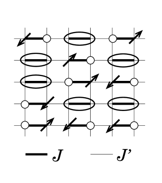
Figure 1: 2D coupled-dimer model with site dilution. The ellipses indicate the formation of local singlets on the intact dimers, open circles indicate vacancies, and arrows represent local moments.

II Models and Numerical Method

We consider a two-dimensional $S=1/2$ Heisenberg antiferromagnetic model of weakly coupled dimers on a square lattice. Yasudaetal01B ; Matsumotoetal01 The Hamiltonian reads

$${\cal H} = J\sum_{\langle ij\rangle\in{\rm dimers}}\epsilon_{i}\epsilon_{j}{\bm{S}}_{i}\cdot{\bm{S}}_{j}+J^{\prime}\sum_{\langle lm\rangle\in{\rm inter-dimers}}\epsilon_{l}\epsilon_{m}{\bm{S}}_{l}\cdot{\bm{S}}_{m}$$ (1)

$$- h\sum_{i}\epsilon_{i}\emph{S}^{z}_{i},$$

where $\epsilon$ takes the values 0 or 1 with probabilities $p$ and $(1-p)$, modeling the doping of the system with non-magnetic impurities. The pairs $\langle ij\rangle$ run on the strong dimer couplings $J$, and the pairs $\langle lm\rangle$ on the weaker inter-dimer couplings $J^{\prime}$ - see Fig. 1. In Sec. III and  IV we first focus on the weak-coupling limit, i.e., $J^{\prime}\ll J$. Later, in Sec. V we investigate the entire phase diagram for $J^{\prime}\lesssim J$.

In the clean limit ($p=0$) and at zero magnetic field there is a critical value $(J^{\prime}/J)_{c}\simeq 0.523$ separating the magnetically ordered phase for $J^{\prime}/J>(J^{\prime}/J)_{c}$ from a dimer-singlet phase for $J^{\prime}/J<(J^{\prime}/J)_{c}$.Matsumotoetal01 Hence, for $J^{\prime}\ll J$ the ground state is in a quantum disordered phase with a finite spin gap $\Delta_{0}\approx J-zJ^{\prime}+O(J^{\prime 2})$, where $z$ is the coordination number for the dimers. This gap can be overcome by a magnetic field $h_{c}=\Delta_{0}$, at which a quantum phase transition to an antiferromagnetically ordered phase occurs. This phase transition is well described by the picture of Bose-Einstein condensation of triplet quasiparticles. Nikunietal00 ; Matsumotoetal04

In a randomly doped system ($p>0$), the zero-field ground state deviates strongly from a dimer singlet. As described in the introduction, any arbitrarily small (but finite) site dilution with concentration $p$ creates an interacting random network of LMs which orders at $T=0$. Laflorencieetal04 When looking at the physics of the system for energies much below the gap $\Delta_{0}$, and consequently for fields $h\ll\Delta_{0}$, the behavior of the diluted system Eq. (1) can be captured by an effective spin-$1/2$ Heisenberg model for the random network of LMs, whose Hamiltonian reads

$$H=\sum_{i<j}J^{\rm(eff)}_{ij}{\bm{S}}_{i}\cdot{\bm{S}}_{j}-h\sum_{i}\emph{S}^{z}_{i}.$$ (2)

Here the ${\bm{S}}$ operators represent $S=1/2$ LMs, exponentially localized around the sites of unpaired spins. Hence, on a $L\times L$ lattice the number of effective spins is approximately $N_{s}=pL^{2}$ (ignoring the case in which a dimer is fully replaced by the impurities, and which does not produce any LM). Since the diluted sites are randomly located throughout the system in Eq. (1), in the effective model Eq. (2) the LMs are also assumed to be randomly distributed on the square lattice. The effective interactions $J^{\rm(eff)}_{ij}$ between LMs $r_{ij}$ take the asymptotic form for large inter-moment distance SigristF96 ; Mikeskaetal04 ; Roscilde06

$$J^{\rm(eff)}_{ij}=(-)^{|i-j|-1}\frac{J_{1}}{r_{ij}^{\alpha}}e^{-r_{ij}/\xi_{0}},$$ (3)

where $J_{1}$ is a parameter determined by $J$ and $J^{\prime}$ of the original diluted model. $\xi_{0}\sim\Delta_{0}^{-1}$ is the correlation length of the gapped ground state in the clean limit. $J^{\rm(eff)}_{ij}$ has ferromagnetic /antiferromagnetic character depending on whether the sites $i$ and $j$ belong to the same/different sublattices; hence the couplings are not frustrated, and they favor AFLRO of the LMs. $\alpha$ is a dimension-dependent exponent, taking values $\alpha=0$ (1D), $\alpha=1$ (2D), and $\alpha=3/2$ (3D). In the following we will concentrate on the 2D case. When $r_{ij}=1$ we need to recover the limit $J^{\rm(eff)}_{ij}=J_{1}e^{-1/\xi_{0}}=J^{\prime}$ for the direct interaction of two unpaired spins through a $J^{\prime}$ coupling. This leads to the identification $J_{1}=J^{\prime}e^{1/\xi_{0}}$, which in turn implies

$$J^{\rm(eff)}_{ij}=(-)^{|i-j|-1}\frac{J^{\prime}}{r_{ij}}e^{-(r_{ij}-1)/\xi_{0}}.$$ (4)

Actually the second-order perturbation calculation which delivers the asymptotic form of the effective couplings, Eq. (3), gives $J_{1}\sim(zJ^{\prime})^{2}/J$; this means that the choice $J_{1}\sim J^{\prime}$, which correctly reproduces the short-range behavior of the effective couplings, leads to an overestimation of such couplings in the long-distance limit. Such an overestimation is nonetheless irrelevant, given the exponential suppression of $J^{\rm(eff)}_{ij}$ at large inter-moment distances.

In the following, we apply the Stochastic Series Expansion (SSE) quantum Monte Carlo (QMC) SyljuasenS02 to both the original and effective Hamiltonians, given by Eq. 1 and  2, in order to investigate the evolution of the ground state of the system as a function of the applied magnetic field. For the effective model with $N_{s}$ randomly distributed spins and non-frustrated long-range exchange interactions, the SSE approach has the advantage of requiring a computational effort $O(N_{s}\ln N_{s})$ instead of the naive $O(N_{s}^{2})$. Sandvik03 To efficiently reach the ground-state behavior via the finite-temperature SSE we make use of a $\beta$-doubling approach Sandvik02A up to an inverse temperature $\beta J=2^{15}$. The full statistics of the disorder distribution is well reproduced by averaging all results over $\approx 300$ disorder realizations.

In the presence of an applied magnetic field, spontaneous AFLRO is reflected by the appearance of a finite transverse staggered magnetization, estimated as

$$m_{s}=\sqrt{S^{\bot}(\pi,\pi)/L^{2}},$$ (5)

where $L$ is the linear system size and $S^{\bot}(\pi,\pi)$ is the transverse staggered structure factor, defined as

$$S^{\bot}(\pi,\pi)=\frac{1}{2L^{2}}{\sum_{ij}}(-)^{|i-j|}\langle S_{i}^{x}S_{j}^{x}+S_{i}^{y}S_{j}^{y}\rangle.$$ (6)

The summation runs over all pairs of occupied sites in the original site-diluted model, and it runs over all possible pairs of LMs in the effective spin model. We also estimate the spin stiffness, corresponding to a superfluid density upon spin-to-boson mapping, via the fluctuations of the winding numbers $W_{X,Y}$ of the SSE worldlines along the two lattice directions $X$ and $Y$ PollockC87 :

$$\rho_{s}=\frac{1}{2\beta J}\langle W_{X}^{2}+W_{Y}^{2}\rangle.$$ (7)

III Monte Carlo Results for weakly coupled dimers

In this section we present the QMC results for the full evolution of the ground state of site-diluted weakly coupled dimers upon varying an applied magnetic field. Here we focus on the case of weakly coupled dimers by choosing $J^{\prime}/J=1/4$. In the clean case, this system is far away from the critical point $J^{\prime}_{c}\approx 0.523J$ in zero field, and it exhibits a disordered state with a correlation length $\xi_{0}\approx 1$. When a magnetic field is applied, the clean system experiences a quantum phase transition to a field-induced antiferromagnetically ordered phase at $h_{c1}^{(0)}=\Delta_{0}=0.60(1)J$. Doping with non-magnetic impurities produces LMs. Our choice of $J^{\prime}\ll\Delta_{0}$ guarantees that the energy scale for the interactions between LMs is well separated from the energy scale of interactions for the intact dimers. Hence the application of a weak field $h\ll J$ to the system will exclusively probe the response of LMs, while intact dimers remain essentially frozen in local singlets.

The succession of field-induced phases in the site-diluted system is fully captured by investigating the staggered magnetization, $m_{s}$ (Eq. 5), and the uniform magnetization, $m_{u}=\sum_{i}\langle S_{i}^{z}\rangle/L^{2}$. The former detects the presence of order in the ground state, while the latter probes the low-energy spectrum both in the ordered and in the disordered phase, exhibiting the presence of a triplet gap via magnetization plateaus. The field dependence of these quantities at a dilution concentration $p=1/8$ is shown in Fig. 2. The following succession of phases is observed in the field range $0\leq h<J$: order-by-disorder phase (OBD), disordered-local-moment phase (DLM), plateau phase (PL), Bose glass phase (BG), XY-ordered phase (XY).

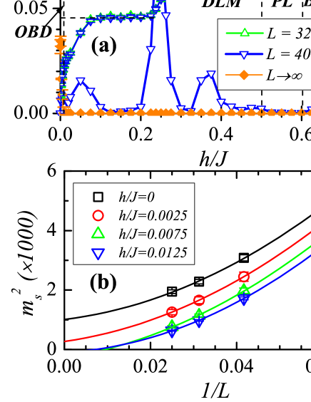
Figure 2: (a): Field dependence of the uniform magnetization, the uniform susceptibility, and the staggered magnetization, of weakly coupled dimers. The coupling ratio is $J^{\prime}/J=1/4$, and the dilution concentration is $p=1/8$. The orange diamonds show the staggered magnetization in the thermodynamic limit, extrapolated by finite-size scaling as shown in (b). OBD: order-by-disorder phase; DLM: disordered-local-moment phase; PL: plateau phase; BG: Bose glass phase; and XY: XY-ordered phase (magnetic condensate).

At zero field, a finite staggered magnetization develops in the system due to the effective interactions among LMs: an extrapolation of the QMC data to infinite size gives $m_{s}=0.032(3)$ (see Fig. 2(b)), indicating that the system is in the OBD phase. Further careful finite-size scaling analysis, discussed in Sec. V, shows that the OBD phase also survives at small finite fields up to $h=h_{\rm DLM}=0.007(1)J\ll J^{\prime}$. At this critical field the uniform magnetization takes the value $m_{u}=0.0208(6)$, namely it is much less than the value $m_{u}^{\rm sat}=pS=1/16$ corresponding to full saturation of the local moments. In fact, the saturation value is only attained at a much higher field $h=h_{\rm PL}\approx 2J^{\prime}$. Hence the ground state of the diluted system at $h_{\rm DLM}<h<h_{\rm PL}$ has a striking feature: the LMs have lost spontaneous ordering transverse to the field, but they are far from being all polarized. In contrast, in a clean antiferromagnet the destruction of a spontaneously ordered state is always accompanied by the full polarization of its constituents. Moreover for $h>h_{\rm DLM}$ the magnetization keeps growing with the field, revealing a gapless spectrum in the absence of spontaneous ordering.

For $h_{\rm PL}<h<\Delta_{0}$ the uniform magnetization remains constant at $m_{u}^{\rm sat}$, indicating a gapped, disordered plateau phase  (PL)Mikeskaetal04 in which the field completely aligns all the unpaired spins, but is not sufficiently strong to break the singlets on strongly coupled dimers. The existence of the PL phase is then a characteristic of the weakly coupled dimer system, and we will see that it disappears when $J^{\prime}\sim\Delta_{0}$.

When $h\geqslant\Delta_{0}$ the gap to excite a triplet in a region of intact dimers (dimer triplet) closes just as it does in the clean system. The reason for this is the finite (albeit exponentially small) probability of finding an arbitrarily large clean region which is devoid of any impurity; the local gap of such a clean region can be arbitrarily close to $\Delta_{0}$ so that a field $h\gtrsim\Delta_{0}$ can create a localized dimer triplet in that region. At variance with the clean system, the field-induced localized quasiparticles do not condense in an extended state with finite superfluid response (spin stiffness), but they are instead localized by disorder and give rise to a quantum disordered Bose glass state. RoscildeH05 ; Roscilde06 In fact the fully polarized LMs act essentially as impenetrable barriers to dimer triplets, while intact dimers close to the non-magnetic impurities have higher local gaps to dimer triplets than in the clean regions. Hence site dilution creates an effective disorder potential which has the effect of Anderson-localizing the dimer triplet quasiparticles appearing in the ground state. Fisheretal89

The resulting BG phase extends over the field range $0.60(1)\leqslant h/J\leqslant 0.67(1)$ in Fig. 2(a), and, similarly to the DLM phase, it is identified by the absence of a gap, as shown by the finite slope in the magnetization curve (namely a finite susceptibility $\chi_{u}=\partial m_{u}/\partial h$). RoscildeH05 ; RoscildeH06 ; Roscilde06

At $h_{\rm BG}/J\approx 0.67$, the applied magnetic field finally drives the system to an XY-ordered antiferromagnetic state. In the picture of bosonic triplet quasiparticles, this magnetically ordered state is a condensate with finite superfluid response. Hence this system realizes a magnetic BG-SF transition, with critical exponents which are quite different from the more conventional Mott insulator to superfluid (MI-SF) transition. RoscildeH05 ; RoscildeH06 ; Roscilde06 As $h$ is increased to reach half filling of the dimer triplets, the behavior of the system is better understood in terms of singlet quasiholes (given that the triplet quasiparticles are effectively hardcore). Such quasiholes experience the reverse succession of phases to that of triplet quasiparticles, namely a transition from XY to BG and then from BG to a plateau phase corresponding to full polarization of the entire sample. RoscildeH05

IV Field-Induced DLM Phase

IV.1 Magnetization curve and effective model

In this section we focus on the unconventional properties of the DLM phase. As already pointed out in the previous section, this phase is characterized by the absence of a gap, as revealed by a finite susceptibility. This is actually not at all obvious from Fig. 2, where the susceptibility appears to nearly vanish in correspondence with intermediate pseudo-plateaus (PP) at $73\%$ and $95\%$ of the saturation magnetization. Only a careful analysis of the temperature scaling of the susceptibility Yuetal08 shows that this quantity remains finite at all field values in the DLM phase down to $T=0$. The first PP extends up to $h\approx 0.7J^{\prime}$; the second appears at $h\approx 1.2J^{\prime}$; and the true saturation plateau is only attained at $h\approx 2J^{\prime}$.

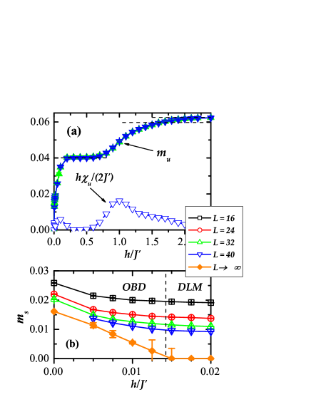
Figure 3: Field dependence of $m_{s}$, $m_{u}$, and $\chi_{u}$ in the effective model, Eq. (2), with $\xi_{0}=1.0$ at a dilution concentration $p=1/8$.

As argued in Sec. II the physics of the site-diluted dimer model at low energy (namely at low fields for $T=0$) can be fully captured by an effective model of coupled LM, Eq. (2). Here we make this statement more quantitative, by directly investigating the physics of the effective model via QMC simulations. The field evolution of the uniform and staggered magnetization for the model of Eqs. (2) and (3) with $\xi_{0}=1$ is shown in Fig. 3. Similarly to the results for the original diluted model, we observe the destruction of the AFLRO phase of the LMs at very small fields, and the occurrence of an extended DLM phase. The occurrence of PPs in the magnetization curve is fully captured in the effective model, albeit with less sharp features. The full qualitative correspondence between the original Hamiltonian and the effective LM model corroborates the picture that the magnetic response of the system up to the plateau phase is dominated by LMs. In the following subsection we will bring this observation to a microscopic level, relating the occurrence of PPs to the quantum magnetic response of LM clusters.

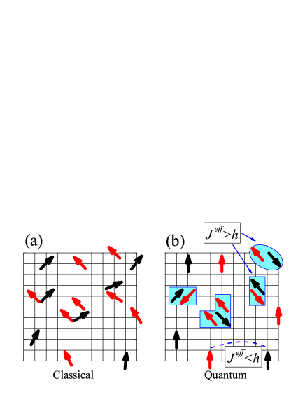
Figure 4: (a): Classical $S\rightarrow\infty$ local moments form a canted antiferromagnetic order at finite field. (b): In the quantum case, neighboring local moments prefer to form strongly correlated states on local clusters, leading to the novel DLM phase. The black and red arrows distinguish spins located on different sublattices.

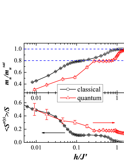
Figure 5: Field dependence of $m_{u}$ and of the transverse spin component $S^{x(y)}$ in the classical effective spin model with $\xi_{0}=1.0$, $p=0.0625$ and $L=40$. The corresponding $m_{u}$ and $m_{s}$ of the quantum model with the same model parameters are also shown for comparison. The staggered magnetization $m_{s}$ of the quantum model has been magnified by a factor of $100$.

IV.2 Quantum nature of the disordered-local-moment phase

In order to emphasize the genuinely quantum character of the DLM phase, in this subsection we focus on a comparison of the system of quantum $S=1/2$ LMs described by Eq. (2) with its classical limit $S=\infty$. The classical limit of Eq. (2) is investigated via a classical Monte Carlo study of a $40\times 40$ lattice with a concentration $p=1/16$ of LMs. The ground state of the classical system is reached by careful thermal annealing with a linear protocol, and results are averaged over typically $500-1000$ configurations.

In the classical limit at $T=0$, the system of randomly distributed LMs in a sufficiently weak magnetic field exhibits a canted antiferromagnetic ground state (Fig. 4(a)). Upon increasing the field, the most isolated LMs minimize their energy by fully aligning with the field, but the remaining LMs preserve long-range order transverse to the field because of the direct long-range effective interactions, as clearly exhibited by Fig. 5. Long-range order is destroyed only when the field exceeds the polarization value of the largest connected LM cluster that can form in the system, thereby polarizing all the LMs. This means that, in the classical limit, the destruction of AFLRO is always accompanied by the full saturation of the magnetization.

Fig. 5 compares the classical behavior with the one of the quantum system with the same concentration of LMs. The uniform magnetization curve shows the emergence of a PP also at the classical level, precisely at the same value as in the quantum case. This result is consistent with the picture (both classical and quantum) of PPs originating from strongly coupled LMs which resist to being fully polarized by the field. This picture relies on the strong inhomogeneity of the network of interacting LMs. This network exhibits an average distance between LMs of $r_{\rm ave}=1/\sqrt{p}$, and a corresponding average coupling $J_{\rm ave}\ll J^{\prime}$ in the limit of diluted LMs. Yet the magnetic response is strongly dominated by the long tails of distribution of LM couplings and not by its average. In particular, there exist small clusters of LMs with linear size $r\ll r_{\rm ave}$, which interact with much stronger couplings $J^{\rm(eff)}\sim J^{\prime}$. The main examples of such clusters are nearest-neighboring dimers and trimers (see the cartoon of Fig. 4(a)). Evidently only a field $h\sim J^{\prime}$ can overcome the antiferromagnetic correlations developing in these clusters.

In the classical limit, LM clusters not only retain short-range antiferromagnetic correlations due to their strong internal coupling, but also long-range correlations due to the direct long-range couplings existing among them. Hence, AFLRO classically survives the strong field $h\sim J^{\prime}$, as shown in Fig. 5. In particular the transverse staggered magnetization shows a PP corresponding to that of the uniform magnetization, a fact which corroborates the above picture.

On the contrary, the quantum mechanical behavior of the LM network is significantly different, as already shown by the data on transverse staggered magnetization in Fig. 2. At the quantum level the presence of strong short-range antiferromagnetic correlations persisting on LM clusters does not coexist with long-range antiferromagnetic correlations between different clusters. In fact a phenomenon of quantum clustering of antiferromagnetic correlations (dimerization, trimerization etc.) turns out to minimize the energy at the quantum level, as sketched in Fig. 4(b). As it will be quantitatively shown in the next subsection, LM dimers have the tendency to freeze in a singlet, LM trimers tend to freeze in a $S_{\rm tot}=1/2$ state aligned with the field, etc. LM dimer singlets are obviously uncorrelated with one another, while LM trimers are also antiferromagnetically uncorrelated because the $S_{\rm tot}=1/2$ state does not reflect the same sublattice structure for all trimers. Hence, except for a small field range slightly above zero field, the entire phase with partially polarized LMs is quantum disordered.

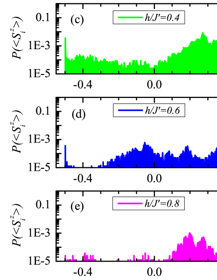
Figure 6: Distribution of the $z$ component of local moments $S_{i}^{z}$ in the effective spin model for classical spins with $\xi_{0}=1.0$, $p=0.0625$, and $L=40$.

IV.3 Local Moment Clusters

The dominant role played by the strongly interacting clusters of LMs in the DLM phase clearly emerges from the distribution of the local magnetization $\langle S_{i}^{z}\rangle$, as well as of the pair correlations $C(r_{ij})=\langle{\bm{S}}_{i}\cdot{\bm{S}}_{j}\rangle$, developed by the inhomogeneous network of LMs. The quantum behavior of these small LM clusters is revealed again by comparison with the classical limit.

The distribution of $\langle S^{z}_{i}\rangle$ in the classical model is shown in Fig. 6. Here the classical spin length is normalized to 1/2 to compare with the quantum case. At zero field, $\langle S^{z}_{i}\rangle$ is obtained by averaging the ordered ground state over all possible orientations. The corresponding probability distribution is:

$$P(\langle S^{z}_{i}\rangle)=\frac{1}{\sqrt{1-\langle S^{z}_{i}\rangle^{2}}}$$ (8)

The presence of a very weak field further enhances two peaks located at $\langle S^{z}_{i}\rangle=\pm 0.5$. The peak at $\langle S^{z}_{i}\rangle=0.5$ corresponds to spins fully polarized by the magnetic field, whereas the peak at $\langle S^{z}_{i}\rangle=-0.5$ corresponds to spins antiferromagnetically coupled to the fully polarized ones (not shown in Fig. 6). For $h/J^{\prime}>0.1$, an extra peak appears at a positive $\langle S^{z}_{i}\rangle$, and it moves towards $\langle S^{z}_{i}\rangle=0.5$ with increasing magnetic field: this peak corresponds to the partially polarized (canted) LMs. At the same time, the peak at $\langle S^{z}_{i}\rangle=-0.5$ drops. This is fully consistent with the picture that classical spins are continuously polarized.

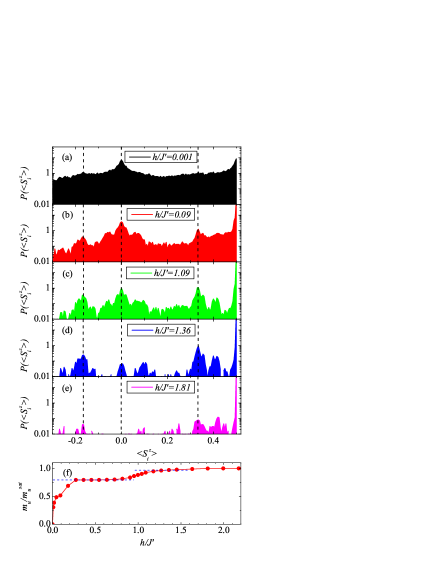
Figure 7: (a)-(e): Distribution of the $z$ component of the local moments $S_{i}^{z}$ in the effective spin model for quantum spins in various fields with $\xi_{0}=1.0$, $p=0.0625$, and $L=40$; (f): Field dependence of the uniform magnetization $m_{u}$ for the same model parameters.

The local magnetization histograms for the quantum system of LMs are shown in Fig. 7, and they exhibit significant differences with respect to the classical case, related to the quantum behavior of LM clusters. For $h=0$ (not shown in Fig. 7) the histogram for $\langle S^{z}_{i}\rangle$ exhibits a unique $\delta$-peak at $\langle S^{z}_{i}\rangle=0$, which obviously corresponds to the fact that the ground state of a quantum Heisenberg antiferromagnet on a finite-size system is a total singlet. The evolution of the local-magnetization histograms is strongly non-monotonic upon applying an increasing field, and it allows to precisely track the succession of phases in the LM network. In fact for a small field, corresponding to the OBD phase, the $\langle S^{z}_{i}\rangle=0$ peak evolves into a broad distribution of local magnetizations, which gives a direct insight into the microscopic structure of the OBD state. A significant portion of the LMs is in a canted antiferromagnetic phase with variable canting, depending on the local structure of LM couplings. This corresponds to the tail of the distribution at $\langle S^{z}_{i}\rangle>0$. At the same time a significant portion of the LMs is fully polarized by the field, as shown by the emergence of a peak at $\langle S^{z}_{i}\rangle=1/2$. These polarized LMs create an effective static field for the LMs which are coupled to them. In the case of antiferromagnetic couplings, this field points opposite to the external field, and it induces a fraction of the LMs to develop a negative local magnetization, as shown by the fat tail of the histogram at $\langle S^{z}_{i}\rangle<0$. Yet the persistence of a central peak at $\langle S^{z}_{i}\rangle=0$ shows that a large fraction of the LMs remains frozen in local singlets, associated with even-number LM clusters (dimers, quadrumers, etc.). At the same time two further peaks clearly emerge in the histogram, at $\langle S^{z}_{i}\rangle=1/3$ and at $\langle S^{z}_{i}\rangle=-1/6$: they can be easily associated with the state $|S_{\rm trimer}=1/2,S^{z}=1/2\rangle$ for LM trimers, where one has a trimer magnetization $S^{z}=\sum_{i\in{\rm trimer}}\langle S^{z}_{i}\rangle=1/3+1/3-1/6=1/2$. Further (and smaller) peaks are to be attributed to larger (and more rare) LM clusters.

The singlet peak at $\langle S^{z}_{i}\rangle=0$ persists over a significant field range. In particular in the field interval $0.3\lesssim h/J^{\prime}\lesssim 0.8$ the local-magnetization histogram changes very little, corresponding to the appearance of the first PPs (as presented in Fig. 7(f)). Only for $h>J^{\prime}$, namely when the field overcomes the largest possible triplet gap associated with a LM dimer-singlet, we observe a decrease of the singlet peak and correspondingly an increase in the slope of the magnetization curve, which allows then to associate the first PP primarily with the quantum magnetic response of LM dimers. Remarkably the LM-trimer peaks at $\langle S^{z}_{i}\rangle=1/3$ and $-1/6$ persist due to the larger gap to full saturation exhibited by these structure. The weak field dependence of such peaks for fields in the interval $1.2\lesssim h/J^{\prime}\lesssim 1.4$ allows then to unambiguously associate the second PP to the LM trimer gap from $|S_{\rm trimer}=1/2,S^{z}=1/2\rangle$ to $|S_{\rm trimer}=3/2,S^{z}=3/2\rangle$, corrected by the local field interacting with each trimer in the network.

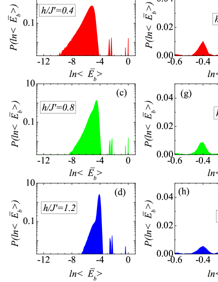
Figure 8: (a)-(d): Distribution of the normalized bond energies $\langle\bar{E_{b}}\rangle$ in the effective spin model with $\xi_{0}=1.0$, $p=0.0625$ and system size $L=40$. (e)-(h): Zoom on the distribution in the region exhibiting the dimer and trimer peaks.

The correspondence of the PP to the magnetic response of LM clusters is further confirmed by investigating the distribution of bond energies. The minimum bond energy is the one of the singlet $E_{b}=-\frac{3}{4}J^{\prime}$. We hence define a normalized bond energy $\bar{E}_{b}=-4E_{b}/(3J^{\prime})$, upper-bounded by 1, and we plot the field dependence of the distribution of $\ln\langle\bar{E}_{b}\rangle$ in Fig. 8. In zero field we observe a very broad distribution, characteristic of a highly inhomogeneous system. In particular there is a very broad peak at low energies (in absolute value), corresponding to the long tail of the distribution of LM couplings. But the most striking feature is a gap between the low-energy peak and two peaks corresponding to the stronger bonds, $\langle\bar{E}_{b}\rangle=1$ and $\langle\bar{E}_{b}\rangle=2/3$. These peaks clearly correspond to dimer singlets and to trimer doublets, respectively. They are very resistant to the application of a field, while the low-energy part of the distribution changes continuously, developing a strong peak which corresponds to the LMs fully polarized by the field. The dimer peak starts to decrease continuously for $h\gtrsim 0.4J^{\prime}$, and it disappears for $h\gtrsim J$, corresponding to the end of the first PP. This in turn reveals that the triplet gaps of the LM dimers follow a distribution, upper bounded by $J^{\prime}$, and due to the effect of the local effective field exerted by the other LMs surrounding the dimer and randomly coupled to it. Therefore the ensemble of LM dimers responds to a field in a continuous fashion, which gives rise to the finite slope of the first PP. Similarly, the trimer peak starts to decrease only for $h\gtrsim 1.2$, consistent with the appearance of the second PP with finite slope.

IV.4 Long-range clusters

A fundamental result in one-dimensional quantum antiferromagnets with random nearest-neighbor couplings is the formation of spin singlets at all energy scales and all distances, to form the so-called random-singlet phase. Fisher94 This phase is fully captured by a real-space renormalization group approach which, at each step, identifies the locally strongest antiferromagnetic bonds and freezes the corresponding spins into a singlet, obtaining then effective couplings for the leftover spins via second-order perturbation theory around the singlet state. The application of a similar approach to the two-dimensional case of the Heisenberg antiferromagnet with random bonds fails to find a random-singlet phase, Linetal03 in agreement with quantum Monte Carlo showing the persistence of Néel order. Laflorencieetal06

The effective model of interacting LMs, Eq. (2), shares similar features to those of a random-bond Heisenberg model, namely the presence of a broad distribution of energy scales for the LM couplings. As shown in this study, and as discussed extensively in Ref. Laflorencieetal04, , the system of LMs in zero field orders antiferromagnetically. We probe directly the possible formation of longer-range singlets by investigating the distribution of the correlation function $C(r_{ij})=\langle{\bm{S}}_{i}\cdot{\bm{S}}_{j}\rangle$ for antiferromagnetically coupled LMs at various inter-moment distances $r_{ij}$. If sites $i$ and $j$ form an approximate singlet, then $C(r_{ij})\approx-3/4$, while if they participate in a long-range trimer, $C(r_{ij})\approx-1/2$. The results for $r_{ij}=1,\sqrt{5},3,\sqrt{13},\sqrt{17}$ in a system with $p=1/16$ are shown in Fig. 9. For $r_{ij}=1$, i.e. for nearest-neighboring moments, there are two sharp peaks in $P(C(r_{ij}))$ around $C(r_{ij})=-3/4$ and $C(r_{ij})=-1/2$ respectively. As discussed above, these two peaks correspond to LMs which participate in nearest-neighboring dimers and trimers. A similar peak structure is also observed for $r_{ij}=\sqrt{5}$ and $r_{ij}=3$, indicating the appearance of similar structures at a larger length scale. The only difference is that the dimer and trimer peaks are weaker and broader, and that there is an extra peak around $C(r_{ij})=0$ for $r_{ij}=\sqrt{5}$ and $r_{ij}=3$, which corresponds to pairs of spins belonging to uncorrelated LM clusters (e.g. two short-range LM dimers or LM trimers). For $r_{ij}>3$ the distribution function completely changes its shape. There is a very broad peak around $C(r_{ij})=0$ and a shoulder around $C(r_{ij})\approx-1/3$, corresponding to long-range AF correlations, but no peaks at $-3/4$ or $-1/2$. It is interesting to notice that the average inter-moment distance $r_{\rm ave}=1/\sqrt{p}=4$ roughly marks the boundary of two behaviors. Hence the above numerical findings imply that at zero field, LMs with inter-moment distance $r_{ij}\lesssim r_{\rm ave}=1/\sqrt{p}$ are generally involved in local singlets (doublets) associated with even (odd) clusters local, and they only marginally take part in the AFLRO. On the contrary the long-range AF correlations are carried by LMs with $r_{ij}\gtrsim r_{\rm ave}$. We finally notice that $J^{\rm(eff)}(r_{ij}=\sqrt{5})\sim h_{\rm DLM}$. Thus, in the DLM phase almost all LMs involved in long-range clusters are fully polarized by the field, and thus the magnetic properties of DLM phase mostly depend on the statistics of the clusters made of nearest-neighboring LMs.

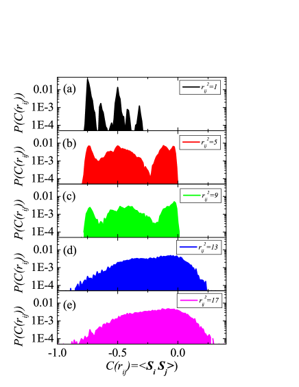
Figure 9: Distribution of inter-moment correlation functions $C(r_{ij})$ for various inter-moment distances $r_{ij}$ in the effective model with $\xi_{0}=1.0$, $p=0.0625$, and at zero field. Here sites $i$ and $j$ are always located on opposite sublattices.

IV.5 Statistics of Local Clusters and Pseudo-Plateaus:
a Minimal Model

As seen in the analysis of the QMC data presented in the previous section, the physics of the DLM phase can be mainly ascribed to the behavior of clusters of nearest-neighboring LMs immersed in the local field which is created by the surrounding isolated LMs. In this section we show how to capture some fundamental aspects of the DLM phase with an elementary model inspired by the above results.

The fundamental assumption we make is the diluteness of the LMs, namely $p\ll 1$. Under this assumption the majority of LMs do not have nearest neighbors, and are typically at a distance $1/\sqrt{p}$ from the other LMs. We will denote these LMs as isolated LMs. Assuming to have an applied magnetic field which is able to polarize most of the isolated LMs, we can essentially neglect the fluctuations of their magnetizations, and treat them as static variables. The remaining minority of LMs is arranged in clusters (dimers, trimers, etc.) which are rare and hence they seldom happen to be close to another. It is therefore a reasonable approximation to neglect all interactions between such clusters. Given that the LMs belonging to the clusters are the only dynamical variables left after freezing the isolated LMs, we can then model the magnetic response of the LM network in the DLM phase as the response of independent LM clusters immersed in the joint external field and in the local field created by the surrounding isolated LMs. For each cluster $C$ we therefore need to diagonalize the following effective Hamiltonian

$${\cal H}_{C}=\sum_{i,j\in C}J_{ij}^{\rm(eff)}{\bm{S}}_{i}\cdot{\bm{S}}_{j}-\sum_{i\in C}\left(h-\sum_{j\in\bar{C}}\frac{J_{ij}^{\rm(eff)}}{2}\right)S^{z}_{i}$$ (9)

where $\bar{C}$ represents the complement to the cluster $C$. In this simplified model we have assumed that all spins outside the clusters are fully polarized, $\langle S^{z}_{j\in\bar{C}}\rangle=1/2$. This is of course not exact due to the existence of other LM clusters, but if they are sufficiently far apart from the cluster under consideration (which is true if $p\ll 1$) we can neglect their couplings $J_{ij}^{\rm(eff)}$ to the cluster $C$, given the exponential decay of $J_{ij}^{\rm(eff)}$ with the distance.

After diagonalizing ${\cal H}_{C}$ for each cluster, we may calculate the uniform magnetization via

$$m_{u}=\sum_{\{C\}}m_{u}(C)P(C),$$ (10)

where $P(C)$ is the probability cluster $C$ appears. Since for each finite cluster $m_{u}(C)$ is a multi-step function at low temperature, $m_{u}$ is expected to exhibit a multi-step character modulated by the distribution $P(C)$.

In Fig. 10(a) the magnetization curve for the effective model with $\xi=1.0$, $p=1/8$, and $L=100$ is calculated by applying Eq. 10. We see that $m_{u}$ reaches the saturated value $m_{u}^{sat}$ only when $h/J^{\prime}\gtrsim 2$. For $h/J^{\prime}\leqslant 2$, the curve resembles the one obtained by QMC, i.e., several PPs can be resolved. By comparing with the magnetization curves of small clusters presented in Fig. 10(b)-(e), we can identify the first PP at $h/J^{\prime}\lesssim 0.7$ to be associated with the $S=0$ singlet states of even-number clusters and the $S=1/2$ states of odd-number clusters. Since $P(C)$ decays exponentially with the cluster size, this PP mostly comes from the $S=0$ state of LM dimers. Similarly we identify that the PP from $1.0\lesssim h/J^{\prime}\lesssim 1.5$ is associated with the $S=1/2$ state of LM trimers. These are consistent with results obtained in previous sections. Interestingly, we can resolve other weak structures in the magnetic curve. For example, the little kinks at $h/J^{\prime}\approx 0.7$ and $h/J^{\prime}\approx 1.7$ are associated with the $S=0$ to $S=1$ and $S=1$ to $S=2$ transitions of four-site chains. We also notice that $m_{u}$ saturates for $h/J^{\prime}\geqslant 2$ for small clusters at least with sizes up to $N=4$. Actually, $N>4$ LM clusters are extremely rare so that they have only negligible contribution to the magnetization curve. Hence we may take $h=2J^{\prime}$ as the saturation field.

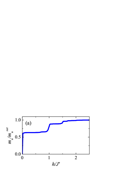
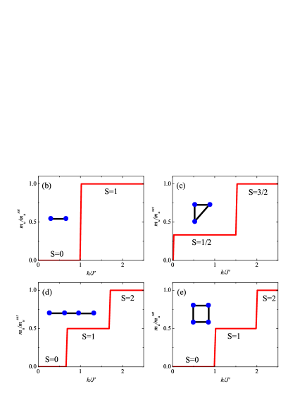
Figure 10: Field dependence of the normalized magnetization $m_{u}/m_{u}^{sat}$ calculated by applying Eq. 10 in the effective model with $\xi_{0}=1.0$, $p=1/8$, and $L=100$ shown in (a). The normalized magnetization on small clusters up to $N=4$ with the same model parameters are also shown in (b)-(e).

We then compare the magnetization curve obtained by diagonalizing LM clusters and then applying Eq. 10 with the one via QMC for the same effective model. The results are presented in Fig. 11 for two values of dilution concentration. We see that the curves obtained by the two different methods agree quite well, especially for the heights and positions of PPs. This agreement confirms that the PPs are ascribed to the distribution of small LM clusters. We notice that the curves from the two methods do not match well for very small $h$, and at $h/J^{\prime}\approx 1$. These discrepancies are closely related to the two assumptions for the LM clusters: since we assume all the single-site LMs are fully polarized by the magnetic field, the first PP calculated by the diagonalization of clusters is expected to appear at very low field. Moreover the interactions among LM clusters, which were neglected in the diagonalization method, lead to smoother transitions between PPs, and to a significant smearing of the second PP. From Fig. 11(b), we see that these features are captured by the QMC simulations, but they are missing in the diagonalization method.

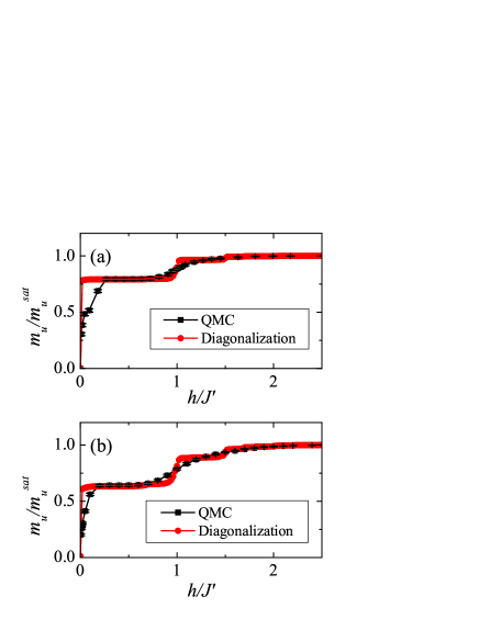
Figure 11: Field dependence of the normalized magnetization $m_{u}/m_{u}^{sat}$ in the effective model with $\xi=1.0$ and $p=1/16$ (in (a)) and $p=1/8$ (in (b)). The results obtained by Eq. 10 (red symbols) for a $L=100$ lattice are compared with those from QMC simulations (black symbols) for a $L=40$ lattice.

IV.6 Bose glass nature of the DLM phase

As seen in the previous subsection, some of the most relevant features of the magnetization curve in the DLM phase can be captured by a model of independent clusters which are storing some LMs not aligned with the field. Upon a standard spin-boson transformation for $S=1/2$ spins, which maps down-spins onto bosons (hereafter called LM quasiparticles) and up-spins onto bosonic holes ($S^{+}\rightarrow b$, $S^{-}\rightarrow b^{\dagger}$, and $S^{z}\rightarrow 1/2-b^{\dagger}b$), the LM Hamiltonian, Eq. (2), takes the following form

$$H=-\sum_{i<j}t_{ij}(b^{\dagger}_{i}b_{j}+b^{\dagger}_{j}b_{i})+\sum_{i<j}V_{ij}n_{i}n_{j}-\sum_{i}\mu_{i}n_{i},$$ (11)

with parameters

$$t_{ij}=\frac{1}{2}|J^{\rm(eff)}_{ij}|~{};$$ (12)

$$V_{ij}=J^{\rm(eff)}_{ij}~{};$$ (13)

$$\mu_{i}=-h-\frac{1}{2}\sum_{j}V_{ij}~{}.$$ (14)

The picture of the DLM phase as dominated by strongly quantum fluctuating LM clusters can be then recast in the bosonic language as a phase in which LM quasiparticles are expelled almost completely from the isolated sites, and they remain localized on the clusters, namely they resonate between two sites on a LM dimer, they localize around the central site of a LM trimer, etc. We then apply the cluster decomposition of the Hamiltonian introduced in the previous subsection, and we neglect inter-cluster couplings in the dilute limit. Neglecting the coupling between clusters and isolated spins as well, we obtain a ground state with isolated sites completely empty of bosons, and clusters hosting one or more boson. Transfering a bosons from a cluster $C$ to an isolated site has a chemical potential price $\Delta\mu\sim\Delta_{C}\sim J^{\prime}$ where $\Delta_{C}$ is the gap to full polarization (or boson depletion) of the cluster. Given that all couplings between the cluster and the isolated spins are smaller than $J^{\prime}$ we can introduce them perturbatively. In doing so, we can still neglect the density-density coupling $V_{ij}n_{i}n_{j}$ with $i\in C$ and $j\in\bar{C}$, because the bosonic occupation of the isolated spins is negligible. The hopping terms $\sim t_{ij}$ for $i\in C$ and $j\in\bar{C}$ lead in turn to a perturbative correction to the wave function of LM quasiparticles, which acquires an exponentially decaying tail (with localization length $\sim|\ln(J_{\rm ave}/J^{\prime})|^{-1}$) over the nearest isolated sites, as it usually happens for a particle in a potential well of depth $\sim\Delta_{C}$.

The resulting picture of exponentially localized LM quasiparticles around the LM cluster locations is hence that of a Bose glass. The density of states of the exponentially localized bosonic states is continuous, and correspondingly an infinitesimal change of the applied field always leads to adding/eliminating one boson, which is a characteristic feature of a Bose glass. This picture will become evident when discussing the complete phase diagram of the system, as shown in the following section.

V Phase Transitions in the 2D Site-Diluted Coupled Dimer System

In this section, we discuss the complete $T=0$ phase diagram of dimer systems with general coupling ratios $0\leqslant J^{\prime}/J\leqslant 1$. This will allow us to give a unified picture of the novel quantum-disordered phases introduced by site dilution in the weakly coupled dimer systems. The main result is that the DLM phase, discussed in details in the previous section, is continuously connected to the Bose glass phase at higher fields. This is further evidence of the Bose glass nature of the DLM phase. Roscilde06 ; RoscildeH05 ; RoscildeH06

V.1 Phase Diagram with Site Dilution

We start by briefly recalling the $T=0$ phase diagram of a coupled-dimer system in the clean limit. At zero field, the ground state is quantum disordered and gapped for weak inter-dimer couplings, and it turns into a Néel-ordered state when the ratio $J^{\prime}/J$ crosses the quantum critical point at $(J^{\prime}/J)_{c}\approx 0.523$. Matsumotoetal01 This critical point belongs to the universality class of the classical three-dimensional Heisenberg model, Matsumotoetal01 ; Chen93 with $\nu=0.71(1)$, $\beta=0.36(1)$, and $z=1$. In the presence of a magnetic field, the critical point at zero field extends to a critical curve in the 2D $(h/J)$-$(J^{\prime}/J)$ plane (see dashed line in Fig. 12). This curve separates the quantum disordered phase at low field and low inter-dimer coupling from the AFLRO phase. For this two-dimensional system, the universality class of this transition is the mean-field one ($\nu=1/2,\beta=1/2$, etc.) with $z=2$. Fisheretal89 ; Sachdev99

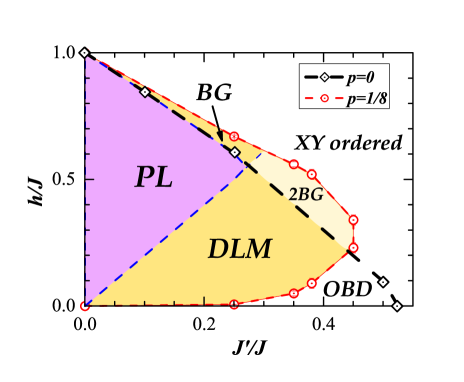
Figure 12: Phase diagram of a site-diluted coupled dimer system at a dilution concentration $p=0.125$. Three distinct phases are shown: the gapped plateau (PL) phase, corresponding to a bosonic Mott insulator; the disordered-local-moment (DLM) phase, corresponding to a Bose glass of LM quasiparticles; Bose glass (BG) phase of dimer triplets, and the two-BG phase, corresponding to a coexistence of LM-quasiparticle and dimer-triplet BG; and the XY ordered phase, corresponding to a condensate of magnetic quasiparticles. The phase boundary in the clean limit $p=0$ (black dashed line) is also shown for comparison.

Fig. 12 shows the complete phase diagram of the two-dimensional doped system with $p=1/8$. As already mentioned in the introduction, doping with a small concentration of non-magnetic impurities immediately induces antiferromagnetic order in the zero-field ground state for every finite inter-dimer coupling $J^{\prime}$. This is in agreement with the mean-field approach of Ref. Mikeskaetal04, . For a large interval of $J^{\prime}/J\lesssim 0.45$ (comprising the case $J^{\prime}=J/4$ of Sec. III), the system is driven back to a quantum disordered phase upon application of a field $h=h_{\rm DLM}\ll J^{\prime}$. At a higher field $h_{\rm BG}$ $(>\Delta_{0})$, the system experiences a second quantum phase transition back to the ordered phase, as discussed in Refs. RoscildeH05, ; RoscildeH06, ; Roscilde06, . For $J^{\prime}/J\lesssim 0.275$ the disordered phase is actually a multiple one, composed of two gapless regions - a DLM phase at low fields and a BG phase at higher field RoscildeH05 ; RoscildeH06 ; Roscilde06 - and an intermediate gapped plateau phase. The plateau phase is bounded from above by the critical line of the clean system, as expected from the fact that below that line no dimer triplet can appear on the rare regions of intact dimers. The curve that bounds the plateau phase from below, on the contrary, corresponds to $h\simeq 2J^{\prime}$; this is also to be expected as the lower critical field for this phase corresponds to the polarization field for all LM clusters whose inter-LM coupling is $J^{\prime}$, and whose effective polarization field is effectively given by $2J^{\prime}$ (see also the discussion in Sec. IV.5 and in Ref. noteonclusters, ). Hence the two curves bounding the plateau phase from above and from below have opposite slopes, and therefore cross each other at $J^{\prime}/J\lesssim 0.275$, where the plateau phase disappears from the phase diagram, leaving space to a unique, continuous gapless disordered phase for $0.275\lesssim J^{\prime}/J\lesssim 0.45$.

Finally, for $J^{\prime}/J\gtrsim 0.45$ the low-field OBD phase merges with the high-field superfluid phase, marking the disappearance of all quantum-disordered phases in the system. It is remarkable to observe that this happens well below the critical value $J^{\prime}/J=0.523$ which marks the disappearance of the quantum-disordered phase in the clean limit. Hence site dilution of the lattice has the effect of significantly shifting the critical $J^{\prime}/J$ ratio for the existence of a disordered phase in the system, as observed experimentally in Mg-doped TlCuCl₃. Fujisawaetal06

The topology of the phase diagram of Fig. 12 is generic for lattices of weakly coupled antiferromagnetic dimers (without frustration) with a concentration of vacancies that falls below the percolation threshold of the lattice. In particular this phase diagram will apply both to$2D$ and to $3D$ arrays of dimers, which are percolating up to a finite concentration of vacancies. In particular a fundamental feature is that the disordered and gapless phases (DLM, 2BG and BG) are simply connected in the phase diagram, so that they systematically separate the gapped phase of fully polarized LMs from the magnetically ordered phases. In other words, in presence of site dilution there is no direct transition between a spin-gapped phase and a magnetically ordered phase. This particular aspect of the topology of the phase diagram is a general property of that of bosons in a disordered lattice Fisheretal89 ; Gurarieetal09 , with the correspondence between spin-gap phases and Mott-/band-insulating phases, and between magnetically ordered phases and superfluid phases.

When considering vacancy concentrations larger than that studied here (but still below the percolation threshold), one expects the gapless phases (DLM and Bose glass) to grow at the expenses of the plateau phase. The magnetically ordered phase at low fields (OBD phase) will also grow towards larger fields, as a denser network of LMs develops a magnetic order which is more robust to the application of a field. On the other hand, the ordered phase at large fields will instead shrink at the expenses of the Bose glass phase, given that a larger triplet density (namely a larger magnetization) is necessary for the triplet gas to condense when the disorder is higher. It is important to contrast the phase diagram of Fig. 12 with the one presented in Ref. Mikeskaetal04, on the basis of mean-field calculations. In the mean-field phase diagram all the gapless disordered phases, dominated by Anderson localization of triplets and/or moments aligned oppositely to the field, are completely absent. This is easily understandable since Anderson localization cannot be captured at the mean-field level; the gapless nature of the above mentioned phases comes from rare, extended regions which can host gapless excitations, while the typical behavior (captured at the mean-field level) is that of a gapped system.

V.2 Two-species Bose glass

As seen in the previous subsection, the DLM phase and the BG phase are indeed continuously connected, and the DLM phase has a nature which is analogous to that of the BG phase. In Section IV.6 we pointed out that the DLM phase is characterized by exponentially localized quasiparticles corresponding to LMs antiparallel to the field, while the BG phase is characterized by the exponential localization of dimer triplets. For $0.275\lesssim J^{\prime}/J\lesssim 0.45$ localized quasiparticles of both species appear above the transition curve for the clean system (which is the condition for the presence of dimer triplets). The appearance of localized dimer triplets before the LM quasiparticles localized on LM clusters disappear upon increasing the field guarantees the gapless nature of the many-body spectrum throughout the quantum disordered regime. Hence the phase diagram region for $J^{\prime}/J\gtrsim 0.275$ comprised between the two curves $h_{\rm BG}(J^{\prime}/J)$ for the doped system and $h_{\rm c}(J^{\prime}/J)$ for the clean system represents a two-species Bose glass (2BG).

Fig. 13 shows the magnetization curve along a section of the phase diagram ($J^{\prime}/J=0.35$) crossing the 2BG phase. Similarly to the case of weaker inter-dimer coupling thoroughly investigated in this paper, clear PPs, corresponding to LM dimers and trimers, are observed at $m_{u}/m_{u}^{\rm(sat)}\approx 0.73$ and $m_{u}/m_{u}^{\rm(sat)}\approx 0.95$, where $m_{u}^{\rm(sat)}=p/2$ is the saturation magnetization of the LMs. The plateau at $m_{u}^{\rm(sat)}$ is on the contrary completely removed by the appearance of dimer triplets at a field $h_{c}(J^{\prime}/J)\approx 0.4J$, which marks the onset of the 2BG phase.

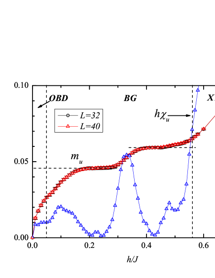
Figure 13: Field evolution of the uniform magnetization $m_{u}$ and the uniform susceptibility $\chi_{u}$ in the site-diluted dimer systems with $J^{\prime}/J=0.35$ and $p=1/8$. Although there is no true magnetization plateau, two pseudo-plateaus $m_{u}/m_{u}^{\rm sat}\approx 0.73$ and $m_{u}/m_{u}^{\rm sat}\approx 0.95$ are resolved.

V.3 Quantum Scaling and Critical Exponents

Next we investigate the properties of the quantum critical line separating the quantum disordered phase from the ordered phase in the phase diagram of Fig. 12. As already pointed out above, for weak inter-dimer coupling ($J^{\prime}\ll J$) this critical line divides ordered and disordered phases which have a different nature when considering the low-field or the intermediate-field region. At low fields, the critical field ($h_{\rm DLM}$) divides the OBD phase from a DLM phase, while at higher fields, the critical field ($h_{\rm BG}$) divides a BG phase of dimer triplets from a condensate of those triplets (corresponding to an XY ordered antiferromagnetic phase). Hence a fundamental question arises whether the quantum critical curve is characterized by universal critical exponents or not.

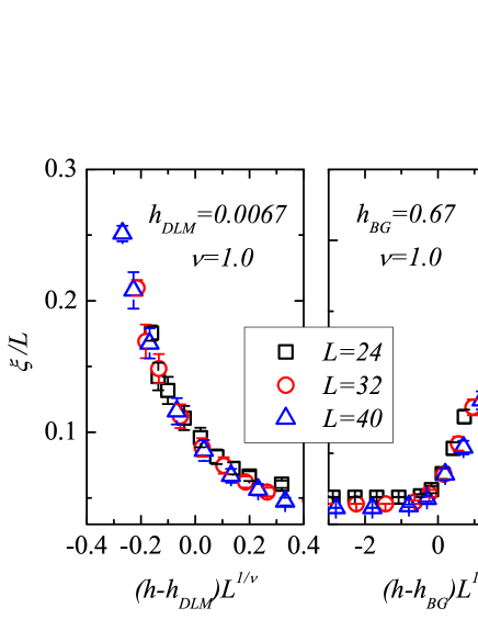
Figure 14: Finite size scaling of the correlation length in the vicinities of the critical fields $h_{\rm DLM}$ (left) and $h_{\rm BG}$ (right). The inter-dimer coupling is $J^{\prime}=J/4$, and the dilution concentration is $p=0.125$.

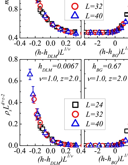
Figure 15: Finite size scaling of the staggered magnetization and the spin stiffness in the vicinities of the critical fields $h_{\rm DLM}$ (left) and $h_{\rm BG}$ (right). The model parameters are the same as in the caption of Fig. 14.

We answer this question by a detailed numerical scaling analysis of the transition line. The correlation length is extracted from the transverse structure factor Eq. (6) by a second-moment method, Cooperetal82 ; Matsumotoetal01 assuming that $S^{\bot}(\vec{k})$ follows a Lorentzian shape close to $\vec{k}=(\pi,\pi)$:

$$\xi=\frac{1}{\Delta k}\sqrt{\frac{S^{\bot}(\pi,\pi)}{S^{\bot}(\pi+\Delta k,\pi)}-1},$$ (15)

where $\Delta k=\frac{2\pi}{L}$. The scaling form of the correlation length is

$$\xi=Lf_{\xi}[L^{1/\nu}(h-h_{c})],$$ (16)

where $f_{\xi}[\cdot]$ denotes the corresponding scaling function. This defines the correlation exponent $\nu$. The scaling plots of the correlation length for $J^{\prime}/J=1/4$ around the two critical fields $h_{\rm DLM}=0.007(1)$ and $h_{\rm BG}=0.67(1)$ are shown in Fig. 14, and they both show the best collapse for an exponent $\nu\approx 1.0(1)$.

To further characterize the universality class of the transition we consider the scaling properties of the staggered magnetization and spin stiffness, whose scaling forms are

$$m_{s}=L^{-\beta/\nu}f_{m_{s}}[L^{1/\nu}(h-h_{c})],$$ (17)

$$\rho_{s}=L^{-(D+z-2)}f_{\rho_{s}}[L^{1/\nu}(h-h_{c})].$$ (18)

Here $\beta$ is the order parameter exponent, $z$ is the dynamical exponent, and $D=2$ is the spatial dimension of the system. Fig. 15 shows the associated scaling plots, which give best collapse for critical fields $h_{\rm DLM}$ and $h_{\rm BG}$ and for a correlation exponent $\nu$ all consistent with the values estimated via the scaling of the correlation length. Moreover we extract the other exponents $\beta=0.9(1)$ and $z=2.0(1)$ at both $h_{\rm DLM}$ and $h_{\rm BG}$.

For a BG-SF transitions, it was theoretically predicted that $z=D=2$, Fisheretal89 in agreement with our results. Moreover for a well defined transition to occur in a disordered system the correlation length exponent $\nu$ must satisfy the Harris criterion Chayesetal86 $\nu\geqslant 2/D=1$, which is also verified by our results. Repeating the same scaling analysis along the critical line of the phase diagram we obtain analogous estimates for the critical exponents, as shown explicitly in Fig. 16 for the case $J^{\prime}/J=0.35$; this is indeed a non-trivial result, as the BG phase close to $h_{\rm BG}$ in this case is a 2BG, as discussed in Section V.2, and across the transition at $h_{\rm BG}$ the dimer triplets condense, while the LM quasiparticles remain localized.

Hence all the above results point towards a critical curve with universal critical exponents defining the SF-BG quantum phase transition in $D=2$. The exponents $\beta$, $\nu$ and $z$ are fully consistent with those estimated in Ref. Roscilde06, for the SF-BG transition in a differently coupled-dimer system (a strongly coupled bilayer) with site dilution, and therefore we argue that they apply to the condensation transition of a generic two-dimensional dirty-boson system with incommensurate particle density.

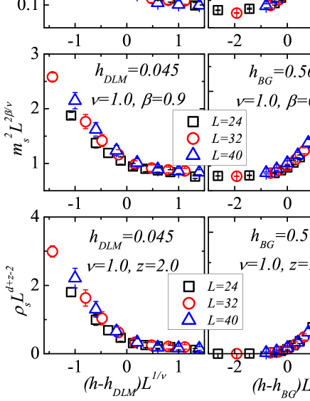
Figure 16: From top to bottom: finite size scaling of correlation length $\xi$, staggered magnetization $m_{s}$, and spin stiffness $\rho_{s}$ at critical fields $h_{\rm DLM}=0.05(1)$ (left) and $h_{\rm BG}=0.56(1)$ (right) in the site-diluted coupled dimers with $J^{\prime}/J=0.35$ and $p=1/8$.

VI Conclusions

Making use of Stochastic Series Expansion Quantum Monte Carlo, we systematically investigated the zero-temperature phase diagram of weakly coupled dimers of $S=1/2$ spins with site dilution and in the presence of a magnetic field. We focused our attention on the specific case of a planar array of coupled dimers. In particular we find that the phase diagram is much richer than the clean system, and also richer than what has been predicted at the mean-field level Mikeskaetal04 . In particular, we show that the impurity-induced ordered state of localizes moments (LMs) at zero field is destroyed by a tiny field for sufficiently small dilution, and that the field drives the system to a novel, disordered-local-moment (DLM) phase, which extends over a very large field range. We elucidate the microscopic nature of this gapless and quantum-disordered phase by comparing results for the diluted coupled-dimer array with those obtained for a network of $S=1/2$ LMs interacting via effective couplings exponentially decaying with the distance. We observe that the DLM phase is characterized by the fact that spins pointing oppositely to the field remain localized on rare clusters of nearest-neighboring LMs. A spin-to-boson mapping shows that the DLM phase is akin to a Bose glass phase of localized hardcore bosons. In the DLM phase, the magnetization curve of the system shows a hierarchy of pseudo-plateaus marking each the full polarization of a class of LM clusters (dimers, trimers, etc.). The specific quantum nature of the DLM phase is revealed by direct comparison with data for the classical limit of the LM network.

A systematic study of the phase diagram of the site-diluted planar array of dimers, as a function of the ratio of inter-dimer coupling to intra-dimer coupling and of the strength of the applied field, reveals that the DLM phase is continuously connected to the Bose glass phase occurring at higher fields, and associated with the Anderson localization of triplet quasi-particles appearing on the intact dimers. This continuous disordered and gapless phase separates the gapped phase of fully polarized LMs from the ordered phases – either the impurity-induced phase present also at zero field, or the field-induced ordered phases characterized by condensation of the triplet quasi-particles. This special feature of the phase diagram is consistent with what expected for dirty-boson systems on a lattice. Moreover the critical exponents for the quantum phase transition separating the gapless disordered phases and the ordered phases appear to be same regardless the specific nature of the ordered and disordered phases which are connected by it. This signals the existence of a novel universality class for the Bose glass-to-superfluid transition in 2D with $\nu\approx 1.0$, $z\approx D=2$, and $\beta\approx 0.9$.

The above findings show that the observation of unconventional disordered phases without a gap, induced by disorder, is quite realistic in the context of doped spin-gap antiferromagnets. In fact, recent studies have focused on the properties of the bond-disordered spin ladder IPA-Cu(Cl_x Br_1-x)₃ Gotoetal08 ; Manakaetal08 ; Manakaetal09 ; Hongetal10 , giving the first evidence of a magnetic Bose glass in this system Manakaetal09 ; Hongetal10 . In the context of bond disorder the Bose glass appears as a consequence of localization of triplets induced by intense fields Nohadanietal05 , while no DLM phase is expected. On the other hand, site dilution of the magnetic lattice, realized by non-magnetic doping, would realize a much broader Bose glass region (comprising the DLM phase), to be observed also at small magnetic fields. This is not at all a negligible aspect: indeed the smallness of the field for which the DLM phase sets in (which can be two or more orders of magnitude smaller than the dominant antiferromagnetic coupling) makes the DLM phase observable also in compounds which have a large spin-gap (of the order of 10 K or higher), and for which the physics of spin-triplet condensation is not easily accessible in experiments. A possible candidate compound is the recently investigated spin ladder compound Bi(Cu_1-xZn_x)₂PO₆, Bobroffetal09 featuring a spin gap of $\sim 35$ K with zero doping ($x=0$). Other potential candidates include the spin-ladder compounds $\rm{(C_{5}H_{12}N)_{2}CuBr_{4}}$ Chaboussantetal97 ; Watsonetal01 ; Klanjseketal08 and IPA-CuCl₃ Masudaetal06 with Zn of Mg doping of the Cu ions.

VII Acknowledgement

We thank N. Bray-Ali, L. Ding, T. Giamarchi, W. Li, G. Misguich, P. Sengupta, M. Sigrist, S. Wessel for fruitful discussions. This work is supported by the Department of Energy through grant No. DE-FG02-05ER46240. Computational facilities have been generously provided by the high-performance computing center at USC.

References

- (1) K. Goto, M. Fujisawa, H. Tanaka, Y. Uwatoko, A. Oosawa, T. Osakabe, and K. Kakurai, J. Phys. Soc. Jpn. 75, 064703 (2006).
- (2) T.M. Rice, Science 298, 760 (2002).
- (3) A. Zheludev, cond-mat/0507534.
- (4) Z. Honda, H. Asakawa, and K. Katsumata, Phys. Rev. Lett. 81, 2566 (1998); A. Zheludev, Z. Honda, K. Katsumata, R. Feyerheim, and K. Prokes, Europhys. Lett. 55, 868 (2001); H. Tsujii, Z. Honda, B. Andraka, K. Katsumata, and Y. Takano Phys. Rev. B 71, 014426 (2005).
- (5) G. Chaboussant, M.-H. Julien, Y. Fagot-Revurat, M. Hanson, L. P. Lévy, C. Berthier, M. Horvatić, and O. Piovesana, Eur. J. Phys. B 6, 167 (1998).
- (6) B. C. Watson, V. N. Kotov, M. W. Meisel, D. W. Hall, G. E. Granroth, W. T. Montfrooij, S. E. Nagler, D. A Jensen, R. Backov, M. A. Petruska, G. E. Fanucci, and D. R. Talham, Phys. Rev. Lett. 86, 5168 (2001).
- (7) M. Jaime, V. F. Correa, N. Harrison, C. D. Batista, N. Kawashima, Y. Kazuma, G. A. Jorge, R. Stern, I. Heinmaa, S. A. Zvyagin, Y. Sasago, and K. Uchinokura, Phys. Rev. Lett. 93, 087203 (2004).
- (8) S. E. Sebastian, P. A. Sharma, M. Jaime, N. Harrison, V. Correa, L. Balicas, N. Kawashima, C. D. Batista, and I. R. Fisher, Phys. Rev. B 72, 100404 (2005).
- (9) T. Nikuni, M. Oshikawa, A. Oosawa, and H. Tanaka, Phys. Rev. Lett. 84, 5868 (2000).
- (10) Ch. Rüegg, N. Cavadini, A. Furrer, H.-U. Güdel, K. Krämer, H. Mutka, A. Wildes, K. Habicht, and P. Vorderwisch, Nature 423, 62 (2003).
- (11) Y. Uchiyama, Y. Sasago, I. Tsukada, K. Uchinokura, A. Zheludev, Y. Hayashi, N. Miura, and P. Böni, Phys. Rev. Lett. 83, 632 (1999); T. Masuda, K. Uchinokura, T. Hayashi, and N. Miura, Phys. Rev. B 66, 174416 (2002).
- (12) V. S. Zapf, D. Zocco, B. R. Hansen, M. Jaime, N. Harrison, C. D. Batista, M. Kenzelmann, C. Niedermayer, A. Lacerda, and A. Paduan-Filho, Phys. Rev. Lett. 96 077204 (2006).
- (13) M. Klanjšek, H. Mayaffre, C. Berthier, M. Horvatić, B. Chiari, O. Piovesana, P. Bouillot, C. Kollath, E. Orignac, R. Citro, and T. Giamarchi, Phys. Rev. Lett. 101, 137207 (2008).
- (14) M. Azuma, Y. Fujishiro, M. Takano, M. Nohara, and H. Takagi, Phys. Rev. B 55, R8658 (1997).
- (15) A. Oosawa and H. Tanaka, Phys. Rev. B 65, 184437 (2002); A. Oosawa, M. Fujisawa, K. Kakurai, and H. Tanaka, Phys. Rev. B 67, 184424 (2003).
- (16) T. Giamarchi, C. Rüegg, and O. Tchernyshyov, Nature Phys. 4, 198 (2008).
- (17) I. Affleck, Phys. Rev. B 43, 3215 (1991).
- (18) T. Giamarchi and A. M. Tsvelik, Phys. Rev. B 59, 11398 (1999).
- (19) M. Matsumoto, B. Normand, T. M. Rice, and M. Sigrist, Phys. Rev. Lett. 89, 077203 (2002); Phys. Rev. B 69, 054423 (2004).
- (20) N. Kawashima, J. Phys. Soc. Jpn. 73, 3219 (2004); cond-mat/0502260.
- (21) G. Misguich and M. Oshikawa, J. Phys. Soc. Jpn. 73 3429 (2004).
- (22) S. Wessel, M. Olshanii, and S. Haas, Phys. Rev. Lett. 87, 206407 (2001); S. Wessel, B. Normand, and S. Haas, Phys. Rev. B 69, 220402 (2004); O. Nohadani, S. Wessel, and S. Haas, Phys. Rev. B 72, 024440 (2005).
- (23) E. S. Sørensen, I. Affleck, D. Augier, and D. Poilblanc, Phys. Rev. B. 58, R14701 (1998); T. Nakamura, Phys. Rev. B 59, R6589, (1999); B. Normand and F. Mila, Phys. Rev. B 65, 104411 (2002).
- (24) M. Sigrist and A. Furusaki, J. Phys. Soc. Jpn. 65, 2385 (1996).
- (25) N. Laflorencie, D. Poilblanc, and A. W. Sandvik, Phys. Rev. B 69, 212412 (2004); N. Laflorencie, D. Poilblanc, and M. Sigrist, Phys. Rev. B 71, 212403 (2005).
- (26) E. F. Shender and S.A. Kivelson, Phys. Rev. Lett. 66, 2384 (1991).
- (27) S. Wessel, B. Normand, M. Sigrist, and S. Haas, Phys. Rev. Lett. 86, 1086 (2001).
- (28) O. Nohadani, S. Wessel, and S. Haas, Phys. Rev. Lett. 95, 227201 (2005).
- (29) R. Yu, S. Haas, and T. Roscilde, Europhys. Lett. 89, 10009 (2010).
- (30) T. Roscilde and S. Haas, Phys. Rev. Lett. 95, 207206 (2005).
- (31) T. Roscilde and S. Haas, J. Phys. B 39, S153 (2006).
- (32) T. Roscilde, Phys. Rev. B 74, 144418 (2006).
- (33) R. Yu, T. Roscilde and S. Haas, New J. Phys. 10 013034 (2008).
- (34) H.-J. Mikeska, A. Ghosh, and A. K. Kolezhuk, Phys. Rev. Lett. 93, 217204 (2004).
- (35) C. Yasuda, S. Todo, M. Matsumoto, and H. Takayama, Phys. Rev. B 64, 092405 (2001).
- (36) M. Matsumoto, C. Yasuda, S. Todo, H. Takayama, Phys. Rev. B 65 014407 (2002).
- (37) O. F. Syljuåsen and A. W. Sandvik, Phys. Rev. E 66, 046701 (2002).
- (38) A. W. Sandvik, Phys. Rev. E 68, 056701 (2003).
- (39) A. W. Sandvik, Phys. Rev. B 66, 024418 (2002).
- (40) E. L. Pollock and D. M. Ceperley Phys. Rev. B 36, 8343 (1987).
- (41) M.P.A. Fisher, P. B. Weichman, G. Grinstein, and D. S. Fisher. Phys. Rev. B 40, 546 (1989).
- (42) D. S. Fisher, Phys. Rev. B 50, 3799 (1994).
- (43) Y.-C. Lin, R. Mélin, H. Rieger, and F. Iglói, Phys. Rev. B 68, 024424 (2003).
- (44) N. Laflorencie, S. Wessel, A. Läuchli, and H. Rieger, Phys. Rev. B 73, 060403 (2006).
- (45) K. Chen, A. M. Ferrenberg, and D. P. Landau, Phys. Rev. B 48, 3249 (1993).
- (46) S. Sachdev, Quantum Phase Transitions. Cambridge University Press, Cambridge (1999).
- (47) In fact is the polarization field for a Heisenberg spin chain with couplings , and hence it applies to all clusters with linear geometry. Strictly speaking, clusters with a ladder or a even a planar geometry can occur as well; they feature a larger polarization field ( for a two-leg ladder, for a square lattice) but they occur with a probability which is extremely small in the case of small doping. In fact the probability to find, e.g., a perfect square-lattice cluster with sites is exponentially small in . Moreover, among all the exponentially rare clusters made of nearest-neighboring sites, the square cluster is realized by only one arrangement of the LMs, whereas the quasi-1 clusters can be realized in a number of ways which is exponentially large in . For all practical purposes, if we can consider that clusters with a polarization field are essentially absent in the system, so that represents the lower boundary of the plateau phase. In strict terms, however, the plateau phase is really gapped in the thermodynamic limit only when , corresponding to the field which polarizes the LMs in the (unlikely) case in which they are all arranged to form an infinite square lattice.
- (48) M. Fujisawa, T. Ono, H. Fujiwara, H. Tanaka, V. Sikolenko, M. Meissner, P. Smeibidl, S. Gerischer, and H. A. Graf, J. Phys. Soc. Jpn. 75, 033702 (2006).
- (49) V. Gurarie, L. Pollet, N. V. Prokof’ev, B. V. Svistunov, and M. Troyer Phys. Rev. B 80, 214519 (2009).
- (50) F. Cooper, B. Freedman, and D. Preston, Nucl. Phys. B 210, 210 (1982).
- (51) J. T. Chayes, L. Chayes, D. S. Fisher, and T. Spencer, Phys. Rev. Lett. 57, 2999 (1986).
- (52) T. Goto, T. Suzuki, K. Kanada, T. Saito, A. Oosawa, I. Watanabe, and H. Manaka, Phys. Rev. B 78 054422 (2008).
- (53) H. Manaka, A. V. Kolomiets, and T. Goto, Phys. Rev. Lett. 101 077204 (2008).
- (54) H. Manaka, H. A. Katori, O. V. Kolomiets, and T. Goto, Phys. Rev. B 79 092401 (2009).
- (55) Tao Hong, A. Zheludev, H. Manaka, and L.-P. Regnault, Phys. Rev. B 81 060410 (2010).
- (56) J. Bobroff, N. Laflorencie, L. K. Alexander, A. V. Mahajan, B. Koteswararao, and P. Mendels, Phys. Rev. Lett. 103 047201 (2009).
- (57) T. Masuda, A. Zheludev, H. Manaka, L.-P. Regnault, J.-H. Chung, and Y. Qiu, Phys. Rev. Lett. 96, 047210 (2006).