On the near periodicity of eigenvalues of Toeplitz matrices

1 Introduction

In order to compute the spectrum of a self-adjoint operator $A$ in a Hilbert space $H$ one can approximate $A$ by a sequence of finite-dimensional operators $A_{n}=P_{n}AP_{n}$, $n=1,2,\dots$, where $P_{n}$ are orthogonal projections on finite-dimensional subspaces of $H$ with the property $P_{n}\to I$ in the strong sense as $n\to\infty$. However, it is well known that the operators $A_{n}$ may have eigenvalues which in the limit do not converge to spectral points of $A$. Such eigenvalues are termed spurious eigenvalues and their presence is often described as spectral pollution (see e.g. [3], [5]). The spectral pollution usually happens in spectral gaps of the operator $A$. This phenomenon has been extensively studied both in the abstract setting (see e.g. [7], [4]), and in various special cases (see e.g. [2], [8], [6]). In particular, it was shown in [7], [4], [9], and [5] that the spectral pollution may occur at any point in a gap of the essential spectrum of $A$.

Perhaps, the simplest example illustrating the spectral pollution, is the classical Toeplitz matrix. Let $a$ be a real-valued piecewise continuous function on the interval $[-\pi,\pi)$, and let $P_{n}$ be the orthogonal projection in $L^{2}(-\pi,\pi)$ on the subspace spanned by the exponentials $(2\pi)^{-1/2}e^{-ikx}$, $k=1,2,\dots,n$. We define the Toeplitz operator with the symbol $a$ as

$$T_{n}=T_{n}[a]=P_{n}AP_{n},$$

where $A$ is the operator of multiplication by $a$. If the range of the function $a$ is a disconnected set, then the spurious eigenvalues, in the limit $n\to\infty$, fill in the gaps separating the components of the range. More precisely, it can be inferred from [1] that an open interval $I$ strictly inside the gap contains $W\log n+O(1)$ eigenvalues of $T_{n}$, where $W=W(a,I)$ is an explicitly computable constant. The objective of this note is to study in more detail the spectrum of the Toeplitz matrix for the piecewise constant symbol of the form

$$a(x)=\left\{\begin{array}[]{ll}0,&x\in[-\pi,L),\\ 1,&x\in[L,\pi),\end{array}\right.$$ (1.1)

where $L\in[0,\pi)$. In [5], it was shown numerically that if $Lp=\pi q$ with some (co-prime) integer numbers $p,q$, then the spurious eigenvalues of the operator $T_{n}[a]$ are “nearly periodic” in $n$ with a “period” $\omega=\omega(p,q)$, see formula (2.1) below. Specifically, let $\lambda^{(k)}\in(0,1)$ be an eigenvalue of the matrix $T_{k}[a]$. Then for each of the operators $T_{k+\omega l}[a]$, $l=1,2,\dots$, there exists an eigenvalue $\lambda^{(k+\omega l)}$ such that the difference $\lambda^{(k+\omega(l+1))}-\lambda^{(k+\omega l)}$ tends to zero as $l\to\infty$. Although the convergence rate of the latter was not estimated in [5], graphs of the eigenvalues qualitatively showed a rate which is faster than the logarithmic filling rate of the gap. As an example, Fig. 1 (see [5]) gives a diagram of the numerically computed eigenvalues of $P_{n}AP_{n}$ vs. $n$, with $L=\frac{\pi}{2}$. The symbols “o” and “x” mark the eigenvalues for even and odd $n$ respectively. The diagram clearly suggests periodicity with period $4$.

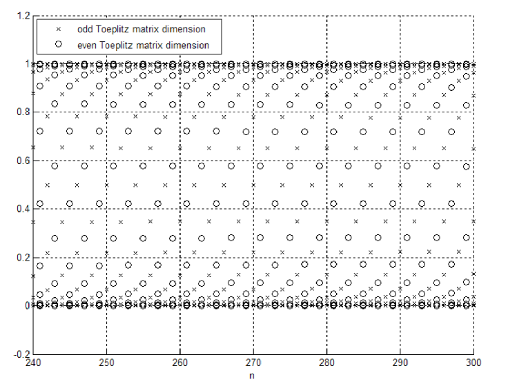
Figure 1: Eigenvalues of $T_{n}[a]$, with $L=\frac{\pi}{2}$, plotted vs. $n$.

The paper [5] (see also [10] in this volume) offered no quantitative measurement of the properties of the periodic behavior. Moreover no rigorous proof has been given, see [10] for some intuitive discussion of the phenomenon.

In this article we address the question of the near periodicity of eigenvalues, but instead of the symbol (1.1) it is more convenient to take $a$ of the form (2.1). We have not been able to find a proof of this effect for the operator $T_{n}[a]$ itself, but we can show its presence for the squared Toeplitz operator, i.e. for $M_{n}[a]=(T_{n}[a])^{2}$, see Theorem 2.1. Numerical examples and more detailed conjectures with regard to the periodicity will be presented in a further publication.

2 The main result

We are concerned with the spectrum of the squared Toeplitz operator

$$M_{n}=M_{n}[a]=(T_{n}[a])^{2}.$$

First, we introduce some consistent notation for eigenvalues of various operators which appear later in the paper. For any self-adjoint matrix operator $S=S_{n}$ of size $n$, we shall denote by $\lambda_{j}(S)$, $j=1,\dots,n$, its eigenvalues labeled in the descending order, and by $\mu_{k}(S)$, $k=1,\dots,n$, its eigenvalues labeled in the ascending order, so that

$$\mu_{j}(S)=\lambda_{n+1-j}(S)\,.$$

Also, for brevity, in the particular case of operators $M_{n}$, we shall write

$$\mu_{j}^{(n)}=\mu_{j}(M_{n})\,,$$

The next theorem is the main result of the paper:

Theorem 2.1.

Let $a(x)$ be the function

$$a(x)=\begin{cases}-1,\ x\in[-\pi,L),\\ 1,\ x\in[L,\pi).\end{cases}$$ (2.1)

with some $L\in[0,\pi)$. Suppose that

$$pL=\pi q$$ (2.2)

for some co-prime $p\in\mathbb{N}$ and $q\in\mathbb{Z}$. Define

$$\omega=\omega(p,q)=\begin{cases}2,\ \ q=0,\\ p,\ \ p\ \ \textup{and}\ q\ \textup{are odd},\\ 2p,\ \ \textup{either}\ p\ \textup{or}\ q\ \textup{is even.}\end{cases}$$

Let $\epsilon\in(0,1)$ be a fixed number, and let $j$ be such that $\mu^{(n)}_{j}<1-\epsilon$. Then for a sufficiently large number $K>0$ and $n\geq K\omega\epsilon^{-1}$,

$$|\mu^{(n)}_{j}-\mu^{(n+\omega)}_{j}|\leq\frac{C\omega(1+\log^{2}n)}{\epsilon n},$$ (2.3)

with a constant $C>0$ independent of $p,q,n,j,\epsilon$.

In general, by $C$ and $c$ we denote various positive constants independent of $n,p,q$ and $\epsilon$, whose precise value is of no importance.

Note that under the condition (2.2) we have

$$\omega(\pi+L)\equiv 0\mod 2\pi.$$ (2.4)

Remark 2.2.

Theorem 2.1 immediately implies that under the condition $\mu^{(n)}_{j}<1-\epsilon$, $\epsilon>0$, for any fixed fixed $N=1,2,\dots$, and all sufficiently large $n$,

$$|\mu^{(n+\omega(m+1))}_{j}-\mu^{(n+\omega m)}_{j}|\leq\frac{C\omega(1+\log^{2}n)}{\epsilon n},$$ (2.5)

for all $m=0,1,\dots,N$, uniformly in $j$. This means that for any $N$ the spectra of $M_{n}[a]$ have strings of length $N$ of “nearly equal” eigenvalues.

Throughout the proof of Theorem 2.1 we omit the subscript $n$ for brevity whenever possible. Denote $Q=Q_{n}=I-P_{n}$ and compute, remembering that $A^{2}=I$:

$$M_{n}[a]=(PAP)^{2}=PAPAP=PA^{2}P-PAQAP=P-PAQAP.$$

This means that

$$\mu^{(n)}_{j}=1-\lambda_{j}(B_{n})\,,$$

where $B_{n}=B_{n}[a]=PAQAP$. Therefore it suffices to prove the inequality (2.3) for the eigenvalues $\lambda_{j}(B_{n})$ which satisfy $\lambda_{j}(B_{n})>\epsilon$, instead.

The entries of the matrix $B_{n}$ are easy to find:

$$b_{rl}=b^{(n)}_{rl}=\frac{1}{2\pi}\sum_{\begin{subarray}{c}m\leq 0,\\ m\geq n+1\end{subarray}}a_{r-m}a_{m-l},\ r,l=1,2,\dots,n,$$ (2.6)

where the Fourier coefficients

$$a_{k}=\frac{1}{\sqrt{2\pi}}\int_{-\pi}^{\pi}a(x)e^{ikx}dx,$$

are given by

$$a_{k}=\left\{\begin{array}[]{ll}-\sqrt{\dfrac{2}{\pi}}L,&k=0,\\[8.5359pt] \sqrt{\dfrac{2}{\pi}}\dfrac{(-1)^{k}}{ik}\left[1-e^{ik(L+\pi)}\right],&k\neq 0.\end{array}\right.$$ (2.7)

The crucial point of our argument is that due to (2.4) the exponential on the right-hand-side of (2.7) is $\omega$-periodic as a function of $k$. This fact is used only once, in the proof of Lemma 2.6.

We need to establish the following theorem.

Theorem 2.3.

Let $a(x)$ be as defined in (2.1), and suppose that the condition (2.2) is satisfied. Let $\epsilon\in(0,1)$ be a fixed number, and let $j$ be such that $\lambda_{j}(B_{n})>\epsilon$. Then for all sufficiently large $n\geq 1$,

$$|\lambda_{j}(B_{n})-\lambda_{j}(B_{n+\omega})|\leq\frac{C\omega(1+\log^{2}n)}{\epsilon n},$$ (2.8)

uniformly in $j$.

First we estimate the entries $b^{(n)}_{rl}$.

Lemma 2.4.

Let $a(x)$ be defined by (2.1), and let $b^{(n)}_{rl}$ be defined by (2.6). Then for all $1\leq l\leq r\leq n$ we have:

$$|b^{(n)}_{rl}|\leq\frac{16}{\pi^{2}}\frac{1+\log n}{|l-r|},\ l\not=r,$$ (2.9)

and

$$|b^{(n)}_{rl}|\leq\frac{8}{\pi^{2}}\biggl{(}\frac{1}{n+1-r}+\frac{1}{l}\biggr{)}.$$ (2.10)

Proof.

Substituting (2.7) in (2.6) we get

$$b_{rl}=-\frac{(-1)^{r-l}}{\pi^{2}}\sum_{\begin{subarray}{c}m\leq 0,\\ m\geq n+1\end{subarray}}\frac{1}{(r-m)(m-l)}\left(1+e^{i(r-l)(L+\pi)}-e^{i(r-m)(L+\pi)}-e^{i(m-l)(L+\pi)}\right).$$ (2.11)

Therefore

$$|b_{rl}|\leq \ \frac{4}{\pi^{2}}\sum_{\begin{subarray}{c}m\leq 0,\\ m\geq n+1\end{subarray}}\left|\frac{1}{(r-m)(m-l)}\right|$$

$$= \ \frac{4}{\pi^{2}}\biggl{(}\frac{1}{|r-(n+1)|\ |(n+1)-l|}+\frac{1}{rl}\biggr{)}+\frac{4}{\pi^{2}}\sum_{\begin{subarray}{c}m\leq-1,\\ m\geq n+2\end{subarray}}\frac{1}{|r-m|\ |m-l|}.$$

The second term can be easily estimated by an appropriate integral. If $r>l$, then

$$\sum_{\begin{subarray}{c}m\leq-1,\\ m\geq n+2\end{subarray}}\frac{1}{|r-m|\ |m-l|}\leq \ \int_{-\infty}^{0}\frac{1}{(r-x)(l-x)}dx+\int_{n+1}^{\infty}\frac{1}{(x-r)(x-l)}dx$$

$$= \ \frac{1}{(r-l)}\biggl{(}\log\left(\frac{n+1-l}{n+1-r}\right)+\log\left(\frac{r}{l}\right)\biggr{)}.$$ (2.12)

The bound (2.9) follows immediately.

Let us derive (2.10). In view of the straightforward bounds

$$\log\left(\frac{n+1-l}{n+1-r}\right)\leq\frac{r-l}{n+1-r},\qquad\log\bigl{(}\frac{r}{l}\bigr{)}\leq\frac{r-l}{l},$$

the right hand side of (2.12) does not exceed

$$\frac{1}{n+1-r}+\frac{1}{l}.$$

For the case $r=l$, a similar estimate can be obtained:

$$\sum_{\begin{subarray}{c}m\leq-1,\\ m\geq n+2\end{subarray}}\frac{1}{|r-m|^{2}}\leq \ \int_{n+1}^{\infty}\frac{1}{(x-r)^{2}}dx+\int_{-\infty}^{0}\frac{1}{(r-x)^{2}}dx$$

$$= \ \frac{1}{n+1-r}+\frac{1}{r}.$$

Hence for all $r\geq l$ we have:

$$|b_{rl}|\leq\frac{8}{\pi^{2}}\biggl{(}\frac{1}{n+1-r}+\frac{1}{l}\biggr{)},$$

which coincides with (2.10). ∎

Let $\omega\in\mathbb{N}$, $1<\omega<n$, and let

$$k=k_{n}=\left\lceil\frac{n}{2}\right\rceil=\begin{cases}\dfrac{n}{2},\quad n\text{ even},\\[5.69046pt] \dfrac{n+1}{2},\quad n\text{ odd}.\end{cases}$$

Let us construct, using matrix $B_{n+\omega}$, two new auxiliary matrices. The $(n+\omega)\times(n+\omega)$-matrix $D_{n+\omega}$ has the entries

$$d^{(n+\omega)}_{rl}=\left\{\begin{array}[]{ll}b^{(n+\omega)}_{rl}&k\leq r<k+\omega,\ \ \textup{or}\ \ \ k\leq l<k+\omega,\\ 0&\hbox{otherwise.}\end{array}\right.$$ (2.13)

The $n\times n$ matrix $F_{n}$ has the entries

$$f^{(n)}_{rl}=\left\{\begin{array}[]{ll}b^{(n+\omega)}_{r,l}&1\leq r\leq k-1,1\leq l\leq k-1,\\[5.69046pt] b^{(n+\omega)}_{r+\omega,l+\omega}&k\leq r\leq n,k\leq l\leq n,\\[5.69046pt] b^{(n+\omega)}_{r,l+\omega}&1\leq r\leq k-1,k\leq l\leq n,\\[5.69046pt] b^{(n+\omega)}_{r+\omega,l}&k\leq r\leq n,1\leq l\leq k-1.\end{array}\right.$$ (2.14)

The method of constructing the matrices $D_{n+\omega}$ and $F_{n}$ from $B_{n+\omega}$ is illustrated by Figure 2. First, we shade the central “cross” of $\omega$ rows and $\omega$ columns in $B_{n+\omega}$, starting with row and column number $k$. The matrix $D_{n+\omega}$ is constructed by replacing everything outside the cross by zeros, and the matrix $F_{n}$ by “removing” the cross, and pulling the remaining four blocks together.

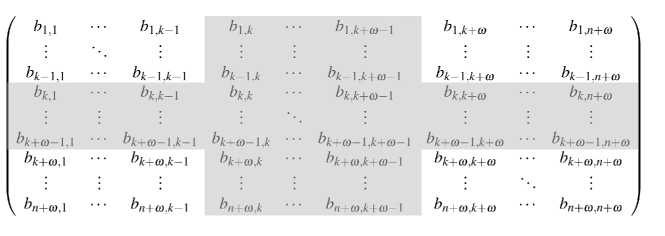
Figure 2: Matrix $B_{n+\omega}$ and the central “cross” used in the construction of matrices $D_{n+\omega}$ and $F_{n}$

Introduce the projections $\Pi_{n,\omega}=P_{k+\omega-1}-P_{k-1}$, and $\Xi_{n,\omega}=P_{n+\omega}(I-\Pi_{n,\omega})$. In terms of these projections, the operator $D^{(n+\omega)}$ can be represented as follows:

$$D_{n+\omega}=\Pi_{n,\omega}B_{n+\omega}\Pi_{n,\omega}+\Pi_{n,\omega}B_{n+\omega}\Xi_{n,\omega}+\Xi_{n,\omega}B_{n+\omega}\Pi_{n,\omega},$$

so that

$$B_{n+\omega}=\Xi_{n,\omega}B_{n+\omega}\Xi_{n,\omega}+D_{n+\omega}.$$

The next lemma estimates the matrix $D_{n+p}$ in terms of these projections.

Lemma 2.5.

Let $b^{(n)}_{rl}$ be defined as in (2.6), and $d^{(n+\omega)}_{rl}$ as in (2.13). Then for any $\epsilon>0$ and all $n\geq p$ we have

$$|(D_{n+p}u,u)|\leq(\epsilon+Cpn^{-1})\|\Pi_{n,p}u\|^{2}+\frac{Cp}{\epsilon}\frac{1+\log^{2}n}{n}\|\Xi_{n,p}u\|^{2},$$ (2.15)

for all $u\in L^{2}(-\pi,\pi)$.

Proof.

Write the straightforward estimate:

$$|(D_{n+\omega}u,u)|\leq \ |(\Pi_{n,\omega}B_{n+\omega}\Pi_{n,\omega}u,\Pi_{n,\omega}u)|+2|(\Pi_{n,\omega}B_{n+\omega}\Xi_{n,\omega}u,\Pi_{n,\omega}u)|$$

$$\leq \ \|\Pi_{n,\omega}B_{n+\omega}\Pi_{n,\omega}\|\ \|\Pi_{n,\omega}u\|^{2}+2\|\Pi_{n,\omega}B_{n+\omega}\Xi_{n,\omega}u\|\ \|\Pi_{n,\omega}u\|$$

$$\leq \ (\|\Pi_{n,\omega}B_{n+\omega}\Pi_{n,\omega}\|+\epsilon)\|\Pi_{n,\omega}u\|^{2}+\epsilon^{-1}\|\Pi_{n,\omega}B_{n+\omega}\Xi_{n,\omega}\|^{2}\|\Xi_{n,\omega}u\|^{2}.$$ (2.16)

Here we have used the elementary estimate $2ab\leq\epsilon a^{2}+\epsilon^{-1}b^{2}$, $\epsilon,a,b>0$.

Let us estimate the matrix norms entering the above inequality. For the first term we estimate the Hilbert-Schmidt norm using the bound (2.10):

$$\|\Pi_{n,\omega}B_{n+\omega}\Pi_{n,\omega}\|_{\mathfrak{S}_{2}}^{2}\leq 2\frac{16^{2}}{\pi^{2}}\sum_{r=k}^{k+\omega-1}\sum_{l=k}^{r}\biggl{(}\frac{1}{n+\omega+1-r}+\frac{1}{l}\biggr{)}^{2}\leq C\frac{\omega^{2}}{k^{2}}.$$ (2.17)

For the matrix $\|\Pi_{n,\omega}B_{n+\omega}\Xi_{n,\omega}\|$ we also estimate its Hilbert-Schmidt norm, but now we need both (2.9) and (2.10):

$$\|\Pi_{n,\omega}B_{n+\omega}\Xi_{n,\omega}\|_{\mathfrak{S}_{2}}^{2}\leq\biggl{(}\sum_{r=k}^{k+\omega-1}\sum_{l=1}^{k-1}+\sum_{r=k+\omega}^{n+\omega}\sum_{l=k}^{k+\omega-1}\biggr{)}|b^{(n+\omega)}_{rl}|^{2}.$$ (2.18)

Let us estimate the first sum, which we denote $S_{1}$. Split it into two parts: $1\leq l\leq k/2$ and $k/2<l\leq k-1$. For the first part we use the estimate (2.9), so that

$$|b^{(n+\omega)}_{rl}|\leq C\frac{1+\log n}{n},$$

and

$$\sum_{r=k}^{k+\omega-1}\sum_{l\leq k/2}|b^{(n+\omega)}_{rl}|^{2}\leq C\frac{(1+\log n)^{2}}{n^{2}}\sum_{r=k}^{k+\omega-1}\sum_{l=1}^{k/2}1\leq C\omega\frac{(1+\log n)^{2}}{n}.$$

The part with $k/2<l\leq k-1$ is estimated with the help of (2.10), so that

$$|b^{(n+\omega)}_{rl}|\leq\frac{C}{n},$$

and

$$\sum_{r=k}^{k+\omega-1}\sum_{k/2<l\leq k-1}|b^{(n+\omega)}_{rl}|^{2}\leq C\frac{\omega}{n}.$$

Thus

$$S_{1}\leq C\omega\frac{(1+\log n)^{2}}{n}.$$

The same bound holds for the second sum on the right hand side of (2.18). Together with (2.17) and (2.16) these bounds lead to the claimed estimate (2.15). ∎

Lemma 2.6.

Suppose that (2.2) is satisfied. Then for all $n\geq 1$ we have

$$\|F_{n}-B_{n}\|\leq\frac{C\omega(1+\log n)}{n}.$$ (2.19)

Proof.

First we estimate the difference $f^{(n)}_{rl}-b^{(n)}_{rl}$. For convenience we re-write the formula (2.6) for $b^{(n+\omega)}_{rl}$:

$$b^{(n+\omega)}_{rl}= \ \frac{1}{2\pi}\sum_{\begin{subarray}{c}m\leq 0,\\ m\geq n+\omega+1\end{subarray}}a_{r-m}a_{m-l}$$

$$= \ \frac{1}{2\pi}\sum_{m\leq 0}a_{r-m}a_{m-l}+\frac{1}{2\pi}\sum_{m\geq n+1}a_{r-m-\omega}a_{m+\omega-l}.$$ (2.20)

Our plan is to estimate the Hilbert-Schmidt norm of $F^{(n)}-B^{(n)}$. So, we estimate carefully the sum of squares $|f_{rl}-b_{rl}|^{2}$ over the four ranges of $r$ and $l$, specified in (2.14).

Case 1: $1\leq r\leq k-1$, $1\leq l\leq k-1$ (upper-left block in Figure 2). According to (2.20) we have

$$f^{(n)}_{rl}-b^{(n)}_{rl}=\frac{1}{2\pi}\sum_{m\geq n+1}\bigl{(}a_{r-m-\omega}a_{m+\omega-l}-a_{r-m}a_{m-l}\bigr{)}.$$

Using (2.7) and (2.4) we get the bound

$$|a_{r-m-p} \ a_{m+p-l}-a_{r-m}a_{m-l}|$$

$$= \ \frac{2}{\pi}|(1-e^{i(r-m)(L+\pi)})(1-e^{i(m-l)(L+\pi)})|\biggl{|}\frac{1}{(r-m-\omega)(m+\omega-l)}-\frac{1}{(r-m)(m-l)}\biggr{|}$$

$$\leq \ \frac{8\omega}{\pi}\biggl{[}\frac{1}{(r-m)^{2}(m-l)}+\frac{1}{(m-r)(m-l)^{2}}\biggr{]}.$$

Therefore, we can estimate:

$$|f^{(n)}_{rl}-b^{(n)}_{lr}|\leq \ \frac{4\omega}{\pi^{2}}\sum_{m\geq n+1}\biggl{[}\frac{1}{(r-m)^{2}(m-l)}+\frac{1}{(m-r)(m-l)^{2}}\biggr{]}$$

$$\leq \ \frac{C\omega}{(n+1-r)(n+1-l)}\leq\frac{C\omega}{n^{2}},\ 1\leq r,l\leq k-1,$$

and hence

$$\sum_{l,r=1}^{k-1}|f^{(n)}_{rl}-b^{(n)}_{rl}|^{2}\leq\frac{C\omega^{2}}{n^{2}}.$$ (2.21)

Case 2: $k\leq r\leq n$, $k\leq l\leq n$ (lower-right block in Figure 2). Using again (2.20), from (2.14) we get:

$$f^{(n)}_{rl}-b^{(n)}_{rl}=\frac{1}{2\pi}\sum_{m\leq 0}\bigl{(}a_{r-m+\omega}a_{m-l-\omega}-a_{r-m}a_{m-l}\bigr{)}.$$

Arguing as in Case 1, we obtain the same bound:

$$\sum_{l,r=k}^{n}|f^{(n)}_{rl}-b^{(n)}_{rl}|^{2}\leq\frac{C\omega^{2}}{n^{2}}.$$ (2.22)

The remaining two cases are trickier:

Case 3: $1\leq r\leq k-1$, $k\leq l\leq n$ (upper-right block in Figure 2). By (2.14),

$$f^{(n)}_{rl}-b^{(n)}_{lr}= \ b^{(n+\omega)}_{r,l+\omega}-b^{(n)}_{lr}$$

$$= \ \frac{1}{2\pi}\sum_{m\leq 0}\bigl{(}a_{r-m}a_{m-l-\omega}-a_{r-m}a_{m-l}\bigr{)}$$

$$\ +\frac{1}{2\pi}\sum_{m\geq n+1}\bigl{(}a_{r-m-\omega}a_{m-l}-a_{r-m}a_{m-l}\bigr{)}.$$

Arguing as in the previous case, we obtain

$$|a_{r-m}a_{m-l-\omega}-a_{r-m}a_{m-l}|\leq \ \frac{8\omega}{\pi}\frac{1}{(r-m)(m-l)^{2}},\ m\leq 0,$$

$$|a_{r-m-\omega}a_{m-l}-a_{r-m}a_{m-l}|\leq \ \frac{8\omega}{\pi}\frac{1}{(r-m)^{2}(m-l)},\ m\geq n+1.$$

We estimate

$$s_{rl}:=\sum_{m\leq 0}\frac{1}{(r-m)(m-l)^{2}}\leq C\frac{1+\log n}{n^{2}},$$

and

$$q_{rl}:=\sum_{m\geq n+1}\frac{1}{(r-m)^{2}(m-l)}\leq C\frac{1+\log n}{n^{2}}.$$

Therefore

$$\sum_{r=1}^{k-1}\sum_{l=k}^{n}s_{rl}^{2}+\sum_{r=1}^{k-1}\sum_{l=k}^{n}q_{rl}^{2}\leq\frac{C(1+\log^{2}n)}{n^{2}}$$

Combining these bounds we arrive at the estimate

$$\sum_{r=1}^{k-1}\sum_{l=k}^{n}|f^{(n)}_{rl}-b^{(n)}_{rl}|^{2}\leq\frac{C\omega^{2}(1+\log^{2}n)}{n^{2}}.$$ (2.23)

Case 4: $k\leq r\leq n$, $1\leq l\leq k-1$ (lower-left block in Figure 2). Since the matrices $F^{(n)}$ and $B^{(n)}$ are Hermitian, we can use the estimate obtained in Case 3, and hence

$$\sum_{r=k}^{n}\sum_{l=1}^{k-1}|f^{(n)}_{rl}-b^{(n)}_{rl}|^{2}\leq\frac{C\omega^{2}(1+\log^{2}n)}{n^{2}}.$$ (2.24)

End of proof. We estimate the norm by the Hilbert-Schmidt norm:

$$\|F_{n}-B_{n}\|\leq\|F_{n}-B_{n}\|_{\mathfrak{S}_{2}}.$$

In view of (2.21), (2.22),(2.23), (2.24),

$$\|F_{n}-B_{n}\|_{\mathfrak{S}_{2}}\leq C\omega\frac{1+\log n}{n},$$

which coincides with the proclaimed estimate. ∎

Our next step is to estimate the difference between eigenvalues of $B_{n+\omega}$ and $F_{n}$. Instead of the eigenvalues themselves, it is more convenient to work with their counting function. Denote by $n_{+}(\lambda,S),\lambda>0,$ the number of eigenvalues of a Hermitian matrix $S$ strictly above $\lambda$.

Lemma 2.7.

Suppose that $\lambda>0$ and $n\geq K\omega\lambda^{-1}$ with a sufficiently large constant $K>0$. Then

$$n_{+}\biggl{(}\lambda+\frac{C\omega}{\lambda}\frac{1+\log^{2}n}{n},F_{n}\biggr{)}\leq n_{+}(\lambda,B_{n+\omega})\leq n_{+}\biggl{(}\lambda-\frac{C\omega}{\lambda}\frac{1+\log^{2}n}{n},F_{n}\biggr{)}.$$

Proof.

We use the projections $\Xi_{n,\omega},\Pi_{n,\omega}$ introduced earlier. Recall that

$$B_{n+\omega}=\Xi_{n,\omega}B_{n+\omega}\Xi_{n,\omega}+D_{n+\omega}.$$

By Lemma 2.5 this implies that

$$B_{n+\omega}\leq \ \Xi_{n,\omega}B_{n+\omega}\Xi_{n,\omega}+\frac{C\omega}{\delta}\frac{1+\log^{2}n}{n}\Xi_{n,\omega}+(\delta+C\omega n^{-1})\Pi_{n,\omega},$$

$$B_{n+\omega}\geq \ \Xi_{n,\omega}B_{n+\omega}\Xi_{n,\omega}-\frac{C\omega}{\delta}\frac{1+\log^{2}n}{n}\Xi_{n,\omega}-(\delta+C\omega n^{-1})\Pi_{n,\omega},$$

for any $\delta>0$. Thus the counting function $n_{+}(\lambda,B_{n+\omega})$ satisfies the following estimates:

$$n_{+}(\lambda,B_{n+\omega})\leq n_{+}\biggl{(}\lambda,\Xi_{n,\omega}B_{n+\omega}\Xi_{n,\omega}+\frac{C\omega}{\delta}\frac{1+\log^{2}n}{n}\Xi_{n,\omega}\biggr{)}+n_{+}(\lambda,(\delta+C\omega n^{-1})\Pi_{n,\omega}),$$ (2.25)

$$n_{+}(\lambda,B_{n+\omega})\geq n_{+}\biggl{(}\lambda,\Xi_{n,\omega}B_{n+\omega}\Xi_{n,\omega}-\frac{C\omega}{\delta}\frac{1+\log^{2}n}{n}\Xi_{n,\omega}\biggr{)},$$ (2.26)

with an arbitrary $\delta>0$. Now take $\delta=\lambda/2$, so that for sufficiently large $K$ under the condition $n\geq K\omega\lambda^{-1}$ we have $\delta+C\omega n^{-1}<\lambda$. Therefore the second term on the right-hand-side of (2.25) equals zero. The matrix $F_{n}$ is obviously similar to $\Xi_{n,\omega}B_{n+\omega}\Xi_{n,\omega}$, so that their positive eigenvalues coincide. Thus (2.25) and (2.26) lead to the required inequalities. ∎

Proof of Theorem 2.3.

By Lemma 2.6, the elementary perturbation theory yields:

$$n_{+}\biggl{(}\lambda+\frac{C\omega(1+\log n)}{n},B_{n}\biggr{)}\leq n_{+}(\lambda,F^{(n)})\leq n_{+}\biggl{(}\lambda-\frac{C\omega(1+\log n)}{n},B_{n}\biggr{)},$$

for any $\lambda\in(0,1]$. Using this bound in combination with Lemma 2.7, we get

$$n_{+}\biggl{(}\lambda+\frac{C\omega}{\epsilon}\frac{1+\log^{2}n}{n},B_{n+\omega}\biggr{)}\leq n_{+}(\lambda,B_{n})\leq n_{+}\biggl{(}\lambda-\frac{C\omega}{\epsilon}\frac{1+\log^{2}n}{n},B_{n+\omega}\biggr{)},$$

for all $\lambda\in[\epsilon,1]$ and $n\geq K\omega\epsilon^{-1}$, with a sufficiently large constant $K$. This means that if $\lambda_{j}(B_{n})>\epsilon$, then

$$|\lambda_{j}(B_{n})-\lambda_{j}(B_{n+\omega})|\leq\frac{C\omega}{\epsilon}\frac{1+\log^{2}n}{n},$$

for all $n\geq K\omega\epsilon^{-1}$. ∎

As we have already pointed out, Theorem 2.1 follows from Theorem 2.3 due to the equality $\mu^{(n)}_{j}=1-\lambda_{j}(B_{n})$.

References

[1]
E.L. Basor,
Trace formulas for Toeplitz matrices with piecewise continuous symbols,
J. Math. Anal. Appl. 120 (1986), no. 1, 25–38.
[2] M. Dauge and M. Suri,
Numerical approximation of the spectra of
non-compact operators arising in buckling problems,
J. of Num. Math, 10, (2002), 193–219.
[3] E. B. Davies and M. Plum, Spectral pollution, IMA J. Numer. Anal.
24 (2004), no. 3, 417–438.
[4] J. Descloux, Essential numerical range of an operator
with respect to a coercive form and
the approximation of its spectrum by the Galerkin Method,
SIAM J. Numer. Anal.,18(6), (1981) 1128–1133.
[5] M. Levitin and E. Shargorodsky, Spectral
pollution and second order relative spectra for self-adjoint operators,
IMA J. Numer. Anal. 24 (2004), no. 3, 393–416.
[6]M. Lewin, E. Séré,
Spectral pollution and how to avoid it
(with applications to Dirac and periodic Schrodinger operators),
to appear in Proc. LMS.
[7] A. Pokrzywa,
Method of orthogonal projections and
approximation of the spectrum of a bounded operator, Studia Math.,
65(1) (1979), 21–29.
[8] J. Rappaz, J. Sanchez Hubert,
E. Sanchez Palencia, and D. Vassiliev,
On spectral pollution in the finite element approximation
of thin elastic ”membrane” shells,
Numer. Math., 75 (1997), 473–500.
[9] E. Shargorodsky, Geometry of higher order relative spectra and projection methods, J. Operator Theory, 44 (2000), 43-62.
[10] E. Shargorodsky, On some open problems in spectral theory, in this volume