Pair HMM based gap statistics for re-evaluation of indels in alignments with affine gap penalties: Extended Version

Abstract

Although computationally aligning sequence is a crucial step in the vast majority of comparative genomics studies our understanding of alignment biases still needs to be improved. To infer true structural or homologous regions computational alignments need further evaluation. It has been shown that the accuracy of aligned positions can drop substantially in particular around gaps. Here we focus on re-evaluation of score-based alignments with affine gap penalty costs. We exploit their relationships with pair hidden Markov models and develop efficient algorithms by which to identify gaps which are significant in terms of length and multiplicity. We evaluate our statistics with respect to the well-established structural alignments from SABmark and find that indel reliability substantially increases with their significance in particular in worst-case twilight zone alignments. This points out that our statistics can reliably complement other methods which mostly focus on the reliability of match positions.

1 Introduction

Having been introduced over three decades ago [22] the sequence-alignment problem has remained one of the most actively studied topics in computational biology. While the vast majority of comparative genomics studies crucially depend on alignment quality inaccuracies abundantly occur. This can have detrimental effects in all kinds of downstream analyses [18]. Still, our understanding of the involved biases remains rather rudimentary [16],[19]. That different methods often yield contradictory statements [9] further establishes the need for further investigations into the essence of alignment biases and their consequences [16].

While the sequence-alignment problem virtually is that of inferring the correct placement of gaps, insertions and deletions (indels) have remained the most unreliable parts of the alignments. For example, Lunter et al. [19], in a whole-genome alignment study, observe 96% alignment accuracy for alignment positions which are far away from gaps while accuracy drops down to 56% when considering positions closely surrounding gaps. They also observe a downward bias in the number of inferred indels which is due to effects termed gap attraction and gap annihilation. Decreased numbers of inferred indels were equally observed in other recent studies [17, 25]. This points out that numbers and size of computationally inferred indels can make statements about alignment quality.

The purpose of this paper is to systematically address such questions. We develop a statistical framework by which to efficiently compute probabilities of the type

$${\mathbb{P}}(I_{d,\mathcal{A}}(x,y)\geq k\,|\,L_{\mathcal{A}}(x,y)=n,\mbox{\rm Sim}_{\mathcal{A}}(x,y)\in[\sigma_{1},\sigma_{2}])$$ (1)

where $(x,y)$ has been randomly sampled from an appropriate pool of protein pairs. In the following pools contain protein pairs which have a (either false or true positive) structural SABMark [28] (see below) alignment. In case of, for example, all pairs of human proteins, (1) would act as null distribution for human. $\mathcal{A}$ is a local or global optimal, score-based alignment procedure with affine gap penalties such as the affine gap cost version of the Needleman-Wunsch (NW) algorithm [22, 14] or the Smith-Waterman (SW) algorithm [30, 32], $L_{\mathcal{A}}(x,y)$ is the length of the alignment, $\mbox{\rm Sim}_{\mathcal{A}}(x,y)$ denotes alignment similarity that is the fraction of perfectly matching and “well-behaved” mismatches vs. ”bad” mismatches (as measured in terms of biochemical affinity [23]) and gap positions. $I_{d,\mathcal{A}}(x,y)$ finally denotes the length of the $d$-th longest gap in the alignment. In summary, (1) can be read as the probability that a NW resp. SW alignment of length $n$ and similarity between $\sigma_{1}$ and $\sigma_{2}$ contains at least $d$ gaps of length $k$ and the reasoning is that gaps which make part of significant such gap combinations are more likely to reflect true indels. Significance is determined conditioned the length $L(x,y)$ of the alignment as well as alignment similarity $\mbox{\rm Sim}(x,y)$. The reasoning behind this is that longer alignments are more likely to accumulate spurious indels such that only increased gap length and multiplicity are significant signs of true indels. Increased similarity $\mbox{\rm Sim}(x,y)$, however, indicates that already shorter and less gaps are more likely to reflect true indels simply because an alignment of high similarity is an overall more trustworthy statement. In summary, we provide a statistically sound, systematic approach to answering questions such as “Am I to believe that $4$ gaps of size at least $6$ in an alignment of length $200$ and similarity $50$ are likely to reflect true indels” as motivated by the recent studies [17, 19, 25].

We opted to address these questions for score-based alignments with affine gap costs for two reasons:

1. To employ score-based such alignments still is a most popular option among most bioinformatics practitioners.

2. Such alignments can be alternatively viewed as Viterbi paths in pair HMMs. While exact statistics on Viterbi paths are hard to obtain and beyond the scope of this study we obtain reasonable approximations by “Viterbi training” sensibly modified versions of the hidden Markov chains which underlie the pair HMMs.

We evaluate our statistics on the well-established SABmark [28] alignments. SABmark is a database of structurally related proteins which cover the entire known fold space. The “Twilight Zone set” was particularly designed to represent the worst case scenario for sequence alignment. While we obtain good results also in the more benign “Superfamilies set” of alignments it is that worst case scenario of twilight zone alignments where our statistics prove their particular usefulness. Here significance of gap multiplicity is crucial while significance of indel length alone does not necessarily indicate enhanced indel quality.

1.1 Related Work

[20] re-evaluate match (but not indel) positions in global score-based alignments by obtaining reliability scores from suboptimal alignments. Similarly, [29] derive reliability scores also for indel positions in global score-based alignments. However, the method presented in [29] reportedly only works in the case of more than 30% sequence identity. Related work where structural profile information is used is [31] whereas [7] re-align rather than re-evaluate.

Posterior decoding algorithms (see e.g. [10, 19, 3] for most recent approaches) are related to re-evaluation of alignments insofar as posterior probabilities can be interpreted as reliability scores. However, how to score indels as a whole by way of posterior decoding does not have a straightforward answer. We are aware of the potential advantages inherent to posterior decoding algorithms—it is work in progress of ours to combine the ideas of pair HMM based posterior decoding aligners with the ideas from this study.

To assess statistical significance of alignment phenomena is certainly related to the vastly used Altschul-Dembo-Karlin statistics [15, 8, 1] where score significance serves as an indicator of protein homology.

To devise computational indel models still remains an area of active research (e.g. [26, 6, 5, 19, 21]). However, the community has not yet come to a final conclusion.

Last but not least, the algorithms presented here are related to the algorithms developed in [27] where the special case of $d=1$ for only global alignments in (2) was treated to explore the relationship of indel length and functional divergence. The advances achieved here are to provide null models also for the more complex case of local alignments and to devise a dynamic programming approach also for the case $d>1$ which required to develop generalized inclusion-exclusion arguments.

Just like in [27] note that empirical statistics approaches fail for the same reasons that have justified the development of the Altschul-Dembo-Karlin statistics: sizes of samples are usually much too small. Here samples (indels in alignments) are subdivided into bins of equal alignment similarity and then further into bins of equal length $n$ and $d$-th longest indel size $k$.

1.2 Summary of Contributions

As above-mentioned, our work is centered around computation of probabilities

$${\mathbb{P}}(I_{d}(x,y)\geq k\,|\,L(x,y)=n,\mbox{\rm Sim}(x,y)\in[\sigma_{1},\sigma_{2}]).$$ (2)

We refer to this problem as Multiple Indel Length Problem (MILP) in the following. Our contributions then are as follows:

1. We are the first ones to address this problem and derive appropriate Markov chain based null models from the pair HMMs which underlie the NW resp. SW algorithms to yield approximations for the probabilities (2).

2. Despite having a natural formulation, the inherent Markov chain problem had no known efficient solution. We present the first efficient algorithm to solve it.

3. We demonstrate the usefulness of such statistics by showing that significant gaps in both global and local alignments indicate increased reliability in terms of identifying true structural indel positions. This became particularly obvious for worst-case twilight zone alignments of at most 25% sequence identity.

4. Thereby we deliver statistical evidence of that computational alignments are biased in terms of numbers and sizes of gaps as described in [19, 25]. In particular too little numbers of gaps can reflect alignment artifacts.

5. Re-evaluation of indels in score-based both local and global alignments had not been explicitly addressed before, in particular, reliable solutions for worst-case twilight zone alignments were missing. Our work adds to (rather than competes with) the above-mentioned related work.

In summary, we have complemented extant methods for score-based alignment re-evaluation. Note that none of the existing methods explicitly addresses indel reliability but rather focus on the reliability of substitutions.

2 Methods

2.1 Pair HMMs and Viterbi Path Statistics

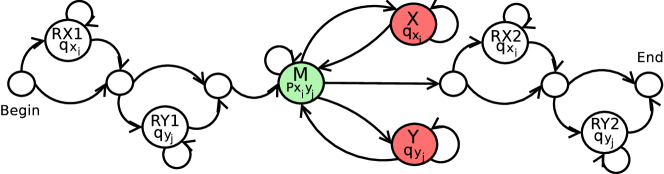
(a) Standard pair HMM

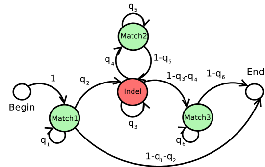
(b) Markov Chain

Figure 1: Standard pair HMM corresponding to local Smith-Waterman alignments and the Markov Chain whose generative statistics, after Viterbi training, approximate the Viterbi statistics of the pair HMM for local alignments.

Figure 2: Markov chain for global alignments. See [27] for details.

In the following we only treat the more complex case of local Smith-Waterman alignments. See [27] for the case of global Needleman-Wunsch like alignments and Fig. 2 for a picture of the corresponding Markov chain. For a treatment of Needleman-Wunsch aligments the Markov chain in Fig. 2 has to be, mutatis mutandis, plugged into the computations of the subsequent subsections.

A local Smith-Waterman alignment with affine gap penalties of two sequences $x=x_{1}...x_{w},y=y_{1}...y_{z}$ is associated with the most likely sequence of hidden states (i.e. the Viterbi path) in the pair HMM of Fig. 1(a) [11]. The path of hidden states translates to an alignment of the two sequences by emitting the necessary symbols along the run. Statistics on Viterbi paths in HMMs pose hard mathematical problems and have not been fully understood. In analogy to [27], we construct a Markov chain whose common, generative statistics mimick the Viterbi statistics of interest here. Hence probabilities derived from this Markov chain serve as approximations of (2). We do this by the following steps:

1. We take the Markov chain of the pair HMM in Fig. 1(a) as a template.

2. We add two match states $M1$, $M3$. The original match state is $M2$.

3. We merge the initial resp. terminal regions into one start resp. end state.

4. We collapse states $X$ and $Y$ into one indel state $I$.

The Markov chain approach is justified by the fact that consecutive runs in Viterbi paths are approximately governed by the geometric distribution which is precisely what a Markov chain reflects. To see this note that to stay with a state in a Viterbi path is, approximately, associated with that a self-transition attains maximum probability in the next step. This depends both on the original transition probability and the backward probability which depends on the observed subsequence to follow starting from that state (see [12], (4.30) and the related discussion). Since it is a general, computational assumption that the background distribution on observed symbols (amino acids) is position-independent Viterbi path transitions can be assumed to be (approximately) position-independent, too. Note that assuming sequence to be position-independent is reflected by that scoring schemes are position-independent. Clearly, this is a computational assumption—we are aware of that the biological reality can be different.

The second point is to take into account the non-stationary character of the original Markov chain. Note that in local alignments, initial and final consecutive stretches of (mis)matches are longer than intermediate (mis)match stretches which translates to $q_{1},q_{6}>q_{5}$ in Fig. 1(a). To see this in more detail, note first that the related discussion in [12] is on stationary HMMs. The non-stationarity of the pair HMM under consideration here is due to that the initial and terminal regions are heavily position-dependent. As a result, the Viterbi paths under consideration have a memory which can contradict the Markov assumption. The most striking effect is that

$${\mathbb{P}}(X_{t+1}=I\,|\,X_{t}=M,X_{t-1}\in\{M,I\})>{\mathbb{P}}(X_{t+1}=I\,|\,X_{t}=M,X_{t-1}=RY1).$$ (3)

which reflects that to open up a gap shortly after having initiated the core alignment tends to be avoided in order to circumvent an early gap penalty. In symbols, this means that it is more likely to postpone the core alignment and see (RY1)(RY1)(RY1) (and, possibly, some more (RX1) before that) than running into an early gap after alignment initiation (RY1)MI. Similar considerations hold for the terminal regions. The second point addresses this by adding initial and terminal match regions M1 and M3 which take the non-stationary character of these areas into account. Point $3$ merely reflects that we are only interested in statistics on alignment regions. Point $4$ finally accounts for that we do not make a difference between insertions and deletions due to the involved symmetry (relative to exchanging sequences).

2.2 Algorithmic Solution of the MILP

We define $C_{n,k,d}$ to be the set of sequences over the alphabet $\mathrm{B,M1,I,M2,M3,E}$ (for Begin, Match1, Indel, Match2, Match3 and End) of length $n$ that contain at least $d$ consecutive $I$ stretches of length at least $k$. Let $A_{n}:=\{X_{n}={\rm M3},X_{n+1}={\rm E}\}$ be the set of sequences with an alignment region of length $n$. We then suggest the following procedure to compute approximations of the probabilities (2) where $T(\sigma_{1},\sigma_{2})$ is supposed to be a pool of protein pairs $(x,y)$ whose alignments exhibit alignment similarity $\mbox{\rm Sim}(x,y)\in[\sigma_{1},\sigma_{2}]$.

1: Compute alignments for all sequence pairs in $T(\sigma_{1},\sigma_{2})$.

2: Infer parameters $q_{1},q_{2},q_{3},q_{4},q_{5},q_{6}$ of the Markov chain by Viterbi training it with the alignments.

3: $n\leftarrow$ length of the alignment of $x$ and $y$

4: Compute ${\mathbb{P}}(C_{n,k,d}\cap A_{n})$ as well as ${\mathbb{P}}(A_{n})$, the probabilities that the Markov chain of Fig. 1(b) generates sequences from $C_{n,k,d}\cap A_{n}$ and $A_{n}$

5: Output

$${\mathbb{P}}(C_{n,k,d}\,|\,A_{n})=\frac{{\mathbb{P}}(C_{n,k,d}\cap A_{n})}{{\mathbb{P}}(A_{n})}$$ (4)

as an approximation for (2).

The idea of step $1$ and $2$ is to specifically train the Markov chain to generate alignments from the pool $T(\sigma_{2},\sigma_{2})$. In our setting, Viterbi training translates to counting $M_{1}$-to-$M_{1}$, $M_{1}$-to-$I$, $I$-to-$I$, $I$-to-$M_{2}$, $M_{2}$-to-$M_{2}$ and $M_{3}$-to-$M_{3}$ transitions in the alignments under consideration to provide maximum likelihood estimates for $q_{1},q_{2},q_{3},q_{4},q_{5}$ and $q_{6}$.

2.3 Efficient Computation of ${\mathbb{P}}(C_{n,k,d}\cap A_{n})$

The problem of computing probabilities of the type (2) has been made the problem of computing the probability that the Markov chain generates sequences from $C_{n,k,d}\cap A_{n}$ and $A_{n}$. While computing

$${\mathbb{P}}(A_{n})={\mathbb{P}}(X_{n}={\rm M_{3}})\cdot{\mathbb{P}}(X_{n+1}={\rm E}\,|\,X_{n}={\rm M_{3}})$$ (5)

is an elementary computation, the question of efficient computation and/or closed formulas for probabilities of the type ${\mathbb{P}}(C_{n,k,d}\cap A_{n})$ had not been addressed in the mathematical literature and poses a last, involved problem.

The approach taken here is related to the one taken in [27], which treated the special case of single consecutive runs (i.e. $d=1$) in the context of the two-state Markov chains which reflect null models for global alignments. We generalize this in two aspects. First, we provide a solution for more than two states (our approach applies for arbitrary numbers of states). Second, we show how to deal with multiple runs.

The probability event design trick inherent to our solution was adopted from that of [24]. The solution provided in [24] can be used for the (rather irrelevant) case of global alignments with linear gap penalties, i.e. gap opening and extension are identically scored. See also [13, 2] for related mathematical treatments of the i.i.d. case.

In the following, let $i,j\in\{\mathrm{B,M_{1},I,M_{2},M_{3},E}\}$ be indices ranging over the alphabet of Markov chain states. Let $e_{i}\in{\mathbb{R}}^{6}$ be the standard basis vector of ${\mathbb{R}}^{6}$ having a $1$ in the i-th component and zero elsewhere. For example, $e_{\rm I}=(0,0,1,0,0,0),e_{{\rm M_{3}}}=(0,0,0,0,1,0)$. We furthermore denote the standard scalar product on ${\mathbb{R}}^{6}$ by $\langle.\,,.\rangle$.

Efficient computation of the probabilities ${\mathbb{P}}(C_{n,k,d}\cap A_{n})$ is obtained by a dynamic programming approach. As usual, we collect the Markov chain parameters (in accordance with Fig. 1(b)) into a state transition probability matrix

$$P=(p_{ij}:={\mathbb{P}}(X_{t}=i\,|\,X_{t-1}=j))_{i,j\in\{\mathrm{B,M1,I,M2,M3,E}\}}=\\ \left(\begin{array}[]{cccccc}0&0&0&0&0&0\\ 1&q_{1}&0&0&0&0\\ 0&q_{2}&q_{3}&1-q_{5}&0&0\\ 0&0&q_{4}&q_{5}&0&0\\ 0&0&0&0&q_{6}&0\\ 0&1-q_{1}-q_{2}&1-q_{3}-q_{4}&0&1-q_{6}&1\end{array}\right)$$ (6)

and an initial probability distribution vector $\pi=e_{B}=(1,0,0,0,0,0)^{T}$. The initial distribution reflects that we start an alignment from the ’Begin’ state. More formally, ${\mathbb{P}}(X_{0}={\rm B})=1$. For example, according to the laws that govern a Markov chain, the probability of being in the indel state I at position $t$ in a sequence generated by the Markov chain is

$${\mathbb{P}}(X_{t}={\rm I})=\langle e_{I},P^{t}\pi\rangle=\langle e_{I},P^{t}e_{B}\rangle.$$ (7)

It can be seen that naive approaches to computing ${\mathbb{P}}(C_{n,k,d}\cap A_{n})$ result in runtimes that are exponential in $n$, the length of the alignments, which is infeasible. Efficient computation of these probabilities is helped by adopting the event design trick of [24]. In detail, we define

$$D_{t,k}:=\{X_{t}={\rm I},...,X_{t+k-1}={\rm I},X_{t+k}\neq{\rm I}\}$$ (8)

to be the set of sequences that have a run of state I of length $k$ that stretches from positions $t$ to $t+k-1$ and ends at position $t+k-1$, that is, the run is followed by a visit of state different from I at position $t+k$.

We further define

$$\pi_{\rm I}:=\frac{1}{(1-p_{{\rm I}\,{\rm I}})}\cdot(p_{{\rm BI}},p_{{\rm M_{1}I}},0,p_{{\rm M_{2}I}},p_{{\rm M_{3}I}},p_{{\rm EI}})^{T}$$ (9)

which can be interpreted as the state the Markov chain is in if we know that the Markov chain has left state I at the time step before. Consider ${\mathbb{P}}(X_{t+s}={\rm I}\,|\,X_{t-1}={\rm I},X_{t}\neq{\rm I})$ as the probability that the Markov chain is in state I at period $t+s$ after having been in the state $\pi_{\rm I}$ at period $t$ (note that this probability is independent of $t$ as we deal with a homogeneous Markov chain). Similarly ${\mathbb{P}}(A_{t+k+s}\,|\,D_{t,k})$ is the probability that the Markov chain transits from state ${\rm M_{3}}$ to state E at position $t+k+s+1$ while it has a run of state I of length $k$ that stretches from positions $t$ to $t+k-1$ and ends at position $t+k-1$. Lastly, we introduce the variables

$$Q_{l,m} := \sum_{1\leq s_{1},...,s_{m}\leq l\atop s_{1}+...+s_{m}=l}{\mathbb{P}}(X_{s_{1}}={\rm I})\prod_{i=2}^{m}{\mathbb{P}}(X_{t+s_{i}}={\rm I}\,|\,X_{t-1}={\rm I},X_{t}\neq{\rm I})$$ (10)

$$R_{L,m} := \sum_{l=m}^{L}Q_{l,m}{\mathbb{P}}(A_{t+k+L-l}\,|\,D_{t,k}),\quad 1\leq m\leq L\leq n$$ (11)

for $1\leq m\leq l\leq n$ where the sum reflects summing over partitions of the integer $l$ into $m$ positive, not necessarily different, integers $s_{i}$. We then obtain the following lemma a proof of which needs a generalized inclusion-exlusion argument.

Lemma 2.1.

$${\mathbb{P}}(C_{n,k,d}\cap A_{n})=\sum_{m=1}^{\lfloor\frac{n}{k+1}\rfloor}(-1)^{m+d}\binom{m-1}{d-1}\cdot{(p_{{\rm II}}^{k-1}(1-p_{\rm II}))}^{m}\cdot R_{n-mk,m}.$$ (12)

Proof: We start by transforming

$$r_{\rm B}(s):={\mathbb{P}}(X_{s}={\rm I})={\mathbb{P}}(X_{s}={\rm I}\,|\,X_{0}={\rm B})=\langle e_{\rm I},P^{s}\pi\rangle,\quad s\geq 1$$ (13)

and

$$\begin{split}r&{}_{\rm I}(s):={\mathbb{P}}(X_{t+s}={\rm I}\,|\,X_{t-1}={\rm I},X_{t}\neq{\rm I})=\frac{{\mathbb{P}}(X_{t-1}={\rm I},X_{t}\neq{\rm I},X_{t+s}={\rm I})}{{\mathbb{P}}(X_{t-1}={\rm I},X_{t}\neq{\rm I})}\\ &=\frac{\sum_{i\neq{\rm I}}{\mathbb{P}}(X_{t-1}={\rm I},X_{t}=i,X_{t+s}={\rm I})}{\sum_{i\neq{\rm I}}{\mathbb{P}}(X_{t-1}={\rm I},X_{t}=i)}=\frac{{\mathbb{P}}(X_{t-1}={\rm I})\sum_{i\neq{\rm I}}{\mathbb{P}}(X_{t}=i,X_{t+s}={\rm I}\,|\,X_{t-1}={\rm I})}{{\mathbb{P}}(X_{t-1}={\rm I})\sum_{i\neq{\rm I}}{\mathbb{P}}(X_{t}=i\,|\,X_{t-1}={\rm I})}\\ &=\frac{{\mathbb{P}}(X_{t-1}={\rm I})\sum_{i\neq{\rm I}}{\mathbb{P}}(X_{t}=i\,|\,X_{t-1}={\rm I}){\mathbb{P}}(X_{t+s}={\rm I}\,|\,X_{t}=i)}{{\mathbb{P}}(X_{t-1}={\rm I})\sum_{i\neq{\rm I}}{\mathbb{P}}(X_{t}=i\,|\,X_{t-1}={\rm I})}\\ &=\frac{\sum_{i\neq{\rm I}}p_{i{\rm I}}\langle e_{\rm I},P^{s}e_{i}\rangle}{\sum_{i\neq{\rm I}}p_{i{\rm I}}}=\frac{1}{1-p_{{\rm I}{\rm I}}}\langle e_{\rm I},P^{s}\sum_{i\neq{\rm I}}p_{i{\rm I}}e_{i}\rangle=\langle e_{\rm I},P^{s}\pi_{\rm I}\rangle\end{split}$$ (14)

According to elementary Markov chain theory, one obtains, where here and in the following $a(k):=p_{{\rm I}{\rm I}}^{k-1}(1-p_{{\rm I}{\rm I}})$

$$\begin{split}{\mathbb{P}}(D_{t,k})&={\mathbb{P}}(X_{t}={\rm I},...,X_{t+k-1}={\rm I},X_{t+k}\neq{\rm I})\\ &={\mathbb{P}}(X_{t}={\rm I})\cdot\prod_{i=1}^{k-1}{\mathbb{P}}(X_{t+i}={\rm I}\,|\,X_{t+i-1}={\rm I})\cdot{\mathbb{P}}(X_{t+k}\neq{\rm I}\,|\,X_{t+k-1}={\rm I})\\ &=r_{\rm B}(t)\cdot p_{{\rm I}{\rm I}}^{k-1}\cdot(1-p_{{\rm I}{\rm I}})\end{split}$$ (15)

and similarly, for $t_{2}\geq t_{1}$

$$\begin{split}{\mathbb{P}}(D_{t_{2},k}\,|\,D_{t_{1},k})&={\mathbb{P}}(D_{t_{2},k}\,|\,X_{t_{1}+k-1}={\rm I},X_{t_{1}+k}\neq{\rm I})\\ &=\begin{cases}r_{\rm I}(t_{2}-t_{1}-k)p_{{\rm I}{\rm I}}^{k-1}(1-p_{{\rm I}{\rm I}})&t_{2}-k>t_{1}\\ 0&t_{2}-k\leq t_{1}\end{cases}\end{split}$$ (16)

Plugging (15) and (16) together yields, for $1\leq t_{1}<...<t_{m}\leq n-k+1$,

$$\begin{split}{\mathbb{P}}(D_{t_{1},k}\cap...\cap D_{t_{m},k})=\begin{cases}{\mathbb{P}}(D_{t_{1},k})\cdot\prod_{i=1}^{m-1}{\mathbb{P}}(D_{t_{i+1}}\,|\,D_{t_{i}})&\forall i:t_{i+1}-t_{i}>k\\ 0&\text{else}\end{cases}\\ =\begin{cases}r_{\rm B}(t_{1})\cdot\prod_{i=1}^{m-1}r_{\rm I}(t_{i+1}-t_{i}-k)\cdot(p_{{\rm I}{\rm I}}^{k-1}(1-p_{{\rm I}{\rm I}}))^{m}&\forall i:t_{i+1}-t_{i}>k\\ 0&\text{else}\end{cases}\\ \end{split}$$ (17)

Including this into the definition of the $Q_{l,m}$ and $R_{L,m}$ yields

$$Q_{l,m}=\sum_{1\leq s_{1},...,s_{m}\leq l\atop s_{1}+...+s_{m}=l}r_{\rm B}(s_{1})\prod_{i=2}^{m}r_{\rm I}(s_{i}),\quad 1\leq m\leq l\leq n$$ (18)

and

$$R_{L,m}=\sum_{l=m}^{L}Q_{l,m}r_{\rm M_{3}}(s_{L-l}).$$ (19)

We now observe that

$$C_{n,k,d}=\cup_{1\leq t_{1}<t_{2}<...<t_{d}\leq n-k+1}(D_{t_{1},k}\cap...\cap D_{t_{d},k}).$$ (20)

and we recall that we would like to compute

$${\mathbb{P}}(C_{n,k,d}\cap A_{n})$$ (21)

where $A_{n}:=\{X_{n}={\rm M_{3}},X_{n+1}={\rm E}\}$ is the set of sequences that have an alignment region of length $n$. Proceeding by inclusion-exclusion yields

$$\begin{split}{\mathbb{P}}(C_{n,k,d}\cap A_{n})&\stackrel{{\scriptstyle(\ref{eq.Cdnk})}}{{=}}{\mathbb{P}}(\cup_{1\leq t_{1}<t_{2}<...<t_{d}\leq n-k+1}(D_{t_{1},k}\cap...\cap D_{t_{d},k}\cap A_{n}))\\ &=\sum_{m=d}^{\lfloor\frac{n}{k+1}\rfloor}K_{m,d}\cdot{\mathbb{P}}(D_{t_{1},k}\cap...\cap D_{t_{m},k}\cap A_{n})\\ &=\sum_{m=d}^{\lfloor\frac{n}{k+1}\rfloor}K_{m,d}\cdot{\mathbb{P}}(D_{t_{1},k}\cap...\cap D_{t_{m},k})\cdot{\mathbb{P}}(A_{n}\,|\,D_{t_{m},k})\end{split}$$ (22)

where $\lfloor\frac{n}{k+1}\rfloor$ reflects the number of non-overlapping events $D_{t_{i}}$, representing subsequences of length $k+1$, that fit into a sequence of length $n$ and

$$K_{m,d}=(-1)^{m+d}\binom{m-1}{d-1}$$ (23)

is a generalized inclusion-exclusion coefficient. While the result can be obtained from considerations that are analogous to that of the usual case $d=1$ (note that $K_{m,1}=(-1)^{m+1}$ just results in the usual inclusion-exclusion), it is not common in the mathematical literature. See the subsequent lemma 2.2 for a formal statement and a proof.

We further define, by computations that are similar to (14),

$$r_{\rm M_{3}}(s):={\mathbb{P}}(A_{t+k+s}\,|\,D_{t,k})\\ ={\mathbb{P}}(X_{t+k+s}={\rm M_{3}}\,|\,D_{t,k})\cdot{\mathbb{P}}(X_{t+k+s+1}={\rm E}\,|\,X_{t+k+s}={\rm M_{3}})=\langle e_{\rm M_{3}},P^{s}\pi_{\rm I}\rangle\cdot p_{{\rm M_{3}}{\rm E}}.$$ (24)

By computations that are analogous to those of [27], where in the following $a(k):=p_{{\rm I}{\rm I}}^{k-1}(1-p_{{\rm I}{\rm I}})$

$$\begin{split}{\mathbb{P}}&(C_{n,k,d}\cap A_{n})\stackrel{{\scriptstyle(\ref{eq.CdnkAn})}}{{=}}\sum_{i=d}^{m}K_{m,d}{\mathbb{P}}(D_{t_{1},k}\cap...\cap D_{t_{m},k})\cdot{\mathbb{P}}(A_{n}\,|\,D_{t_{m},k})\\ &\stackrel{{\scriptstyle(\ref{eq.D3})}}{{=}}\sum_{m=1}^{\lfloor\frac{n}{k+1}\rfloor}K_{m,d}\cdot a(k)^{m}\sum_{1\leq t_{1}<...<t_{m}\leq n-k+1\atop t_{i+1}-t_{i}>k}r_{1}(t_{1})\cdot\prod_{i=1}^{m-1}r_{\rm I}(t_{i+1}-t_{i}-k)\cdot r_{\rm M_{3}}(n-t_{m}-k)\\ &=\sum_{m=1}^{\lfloor\frac{n}{k+1}\rfloor}K_{m,d}\cdot a(k)^{m}\left[\sum_{l=m}^{n-mk}Q_{l,m}\cdot r_{\rm M_{3}}(n-mk-l))\right].\\ &=\sum_{m=1}^{\lfloor\frac{n}{k+1}\rfloor}K_{m,d}\cdot a(k)^{m}\cdot R_{n-mk,m}\\ &=\sum_{m=1}^{\lfloor\frac{n}{k+1}\rfloor}(-1)^{m+d}\binom{m-1}{d-1}\cdot{(p_{{\rm I}{\rm I}}^{k-1}(1-p_{{\rm I}{\rm I}}))}^{m}\cdot R_{n-mk,m}.\end{split}$$ (25)

$\diamond$

Lemma 2.2.

Let $D_{i},i\in\{1,...,N\}$ be a family of $N$ events. Then it holds that

$${\mathbb{P}}(\cup_{1\leq i_{1}<...<i_{d}\leq N}(D_{t_{1}}\cap...\cap D_{t_{d}})=\sum_{m=d}^{N}(-1)^{m+d}\binom{m-1}{d-1}\sum_{1\leq i_{1}<...<i_{m}\leq N}{\mathbb{P}}(D_{i_{1}}\cap...\cap D_{i_{m}}).$$ (26)

Proof. The proof proceeds similarly to that of the special, well known case of $d=1$. Let $\omega\in\cup_{i_{1}<...<i_{d}}(D_{i_{1}}\cap...\cap D_{i_{d}})$ such that, w.l.o.g., $\omega$ is contained in $D_{1},...,D_{n}$ where $n\leq N$, but not contained in $D_{n+1},...,D_{N}$. Let $\mathbf{1}_{\omega}$ be the indicator function of $\omega$. According to the choice of $\omega$ it holds that

$$\mathbf{1}_{\omega}(D_{i})=\begin{cases}1&1\leq i\leq n\\ 0&\text{else}\end{cases}.$$ (27)

Proceeding along the lines of the proof of the usual inclusion-exclusion theorem ($d=1$) (see e.g. [4]) it suffices to show that

$$\mathbf{1}_{\omega}(\cup_{i_{1}<...<i_{d}}(D_{t_{1}}\cap...\cap D_{t_{d}}))=\sum_{m=d}^{n}(-1)^{m+d}\binom{m-1}{d-1}\sum_{J\subset\{1,...,n\}\atop|J|=l}\mathbf{1}_{\omega}(\cap_{j\in J}D_{j})$$ (28)

Evaluating this equation at $\omega$ amounts to showing that

$$1=\sum_{m=d}^{n}(-1)^{n+d}\binom{m-1}{d-1}\binom{n}{m}.$$ (29)

This is done by induction on $d$. The case $d=1$

$$1=\sum_{l=1}^{n}(-1)^{n+1}\binom{m-1}{0}\binom{n}{m}=\sum_{m=1}^{n}(-1)^{n+1}\binom{n}{m}$$ (30)

is the usual case of standard inclusion-exclusion which, by putting the right hand side to the left, follows from

$$\sum_{m=0}^{n}(-1)^{n}\binom{n}{m}=(1-1)^{n}=0.$$ (31)

$d\to d+1$: In this case, In this case, we have to show that

$$\sum_{m=d+1}^{n}(-1)^{n+d+1}\binom{m-1}{d}\binom{n}{m}=1$$ (32)

Therefore, we can assume that

$$\sum_{m=d}^{n}(-1)^{m+d}\binom{m-1}{d-1}\binom{n}{m}=1\quad\Leftrightarrow\quad\sum_{m=d+1}^{n}(-1)^{l+d+1}\binom{m-1}{d-1}\binom{n}{m}=\binom{n}{d}-1.$$ (33)

Furthermore, it holds that

$$\binom{m}{d}\binom{n}{m}=\frac{n!}{m!(n-m)!}\cdot\frac{m!}{d!(m-d)!}=\frac{n!}{d!(n-d)!}\cdot\frac{(n-d)!}{(m-d)!(n-m)!}=\binom{n}{d}\binom{(n-d)}{(m-d)}.$$ (34)

We proceed

$$\begin{split}\sum_{m=d+1}^{n}&(-1)^{n+d+1}\binom{m-1}{d}\binom{n}{m}=\sum_{m=d+1}^{n}(-1)^{n+d+1}[\binom{m}{d}-\binom{m-1}{d-1}]\binom{n}{m}\\ &\stackrel{{\scriptstyle(\ref{eq.iv})}}{{=}}[\sum_{m=d+1}^{n}(-1)^{n+d+1}\binom{m}{d}\binom{n}{m}]-\binom{n}{d}+1\\ &\stackrel{{\scriptstyle(\ref{eq.lknl})}}{{=}}[\sum_{m=d+1}^{n}(-1)^{n+d+1}\binom{n}{d}\binom{(n-d)}{(m-d)}]-\binom{n}{d}+1\\ &=\binom{n}{d}[\sum_{m=d+1}^{n}(-1)^{n+d+1}\binom{(n-d)}{(m-d)}]-\binom{n}{d}+1\\ &=\binom{n}{d}[\sum_{m^{\prime}=1}^{n}(-1)^{n+1}\binom{n}{m^{\prime}}]-\binom{n}{d}+1\\ &\stackrel{{\scriptstyle(\ref{eq.d=1})}}{{=}}\binom{n}{d}-\binom{n}{d}+1=1\end{split}$$ (35)

which concludes the proof. $\diamond$

The consequences can be summarized in the following theorem.

Theorem 2.1.

A full table of values ${\mathbb{P}}(C_{n,k,d}\cap A_{n}),k\leq n\leq N$ can be computed in $O(N^{3})$ runtime.

Proof. Observing the recursive relationship

$$Q_{l,m}=\sum_{s=1}^{l-m+1}{\mathbb{P}}(X_{t+s}={\rm I}\,|\,X_{t-1}={\rm I},X_{t}\neq{\rm I})Q_{l-s,m-1},\quad m>1$$ (36)

yields a standard dynamic programming procedure by which the ensemble of the $Q_{l,m}$ and the $R_{L,m}$ ($1\leq m\leq l,L\leq N$) can be computed in $O(N^{3})$ runtime. This also requires that the values ${\mathbb{P}}(X_{s}={\rm I}),{\mathbb{P}}(X_{t+s}={\rm I}\,|\,X_{t-1}={\rm I},X_{t}\neq{\rm I})$ have been precomputed which can be done in time linear in $N$. After computation of the $Q_{l,m}$ and the $R_{L,m}$, computation of the ${\mathbb{P}}(C_{n,k,d}\cap A_{n}),1\leq k\leq n\leq N$ then equally requires $O(N^{3})$ time which follows from lemma 2.1. $\diamond$

3 Results

Table 1: Markov chain parameters for local alignments.

Twilight Zone (Twi)
Similarity (%)	20 - 30	30 - 40	40 - 50	50 - 60	60 - 70	70 - 80	80 - 90	90 - 100
No. Alignments	-	27	1896	12512	9716	3956	1733	259
$q_{1}$	-	0.9552	0.9606	0.9564	0.9485	0.9364	0.9188	0.9149
$q_{2}$	-	0.0216	0.0300	0.0315	0.0265	0.0167	0.0078	0.0036
$q_{3}$	-	0.7500	0.6667	0.5893	0.4692	0.3210	0.3640	0.0000
$q_{4}$	-	0.0588	0.1948	0.2185	0.1739	0.0979	0.0459	0.0000
$q_{5}$	-	0.8261	0.9439	0.9353	0.9226	0.8999	0.9253	1.0000
$q_{6}$	-	0.9417	0.9514	0.9472	0.9335	0.9077	0.8991	0.7755
Superfamilies (Sup)
Similarity (%)	20 - 30	30 - 40	40 - 50	50 - 60	60 - 70	70 - 80	80 - 90	90 - 100
No. Alignments	-	44	3743	23726	18633	7275	2613	454
$q_{1}$	-	0.9511	0.9584	0.9568	0.9534	0.9528	0.9346	0.9273
$q_{2}$	-	0.0267	0.0330	0.0330	0.0266	0.0160	0.0085	0.0034
$q_{3}$	-	0.7643	0.6829	0.6043	0.5001	0.4044	0.2553	0.0000
$q_{4}$	-	0.0828	0.1962	0.2390	0.2390	0.2220	0.0959	0.0000
$q_{5}$	-	0.8952	0.9430	0.9410	0.9466	0.9674	0.9820	0.0000
$q_{6}$	-	0.9438	0.9508	0.9495	0.9443	0.9504	0.9407	0.7921

Table 2: Markov chain parameters for global alignments.

Twilight Zone (Twi)
Similarity (%)	20 - 30	30 - 40	40 - 50	50 - 60	60 - 70	70 - 80	80 - 90	90 - 100
No. Alignments	31	1811	9156	616	36	7	8	-
$1-2p$	0.9092	0.9290	0.9287	0.9311	0.9528	0.9790	0.9939	-
$q$	0.2615	0.1835	0.1475	0.0994	0.0619	0.0269	0.0364	-
Superfamilies (Sup)
Similarity (%)	20 - 30	30 - 40	40 - 50	50 - 60	60 - 70	70 - 80	80 - 90	90 - 100
No. Alignments	44	2925	17127	3234	1304	454	39	-
$1-2p$	0.9054	0.9277	0.9292	0.9421	0.9630	0.9788	0.9900	-
$q$	0.2528	0.1876	0.1482	0.0980	0.0523	0.0257	0.0097	-

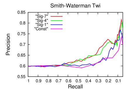
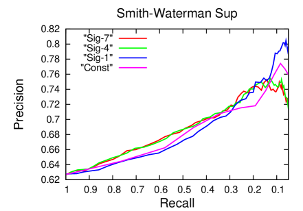
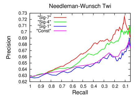
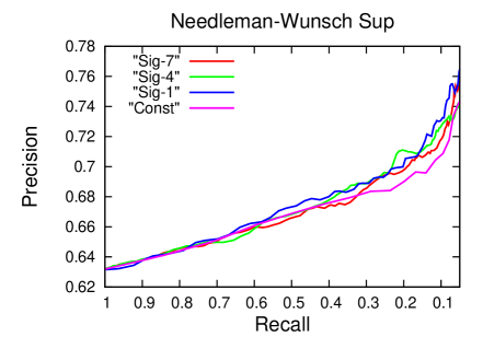
Figure 3: Precision-Recall curves for the different sets of computational alignments. Recall is lowered through lowering the significance threshold $\theta$ for the strategies ${\rm Sig_{D}}(\theta)$ ($\theta=1.0$ for maximal recall of $1.0$) and for raising indel length in the baseline strategy Const (length = $1$ for maximal recall of $1.0$).

Data

We downloaded both the “Superfamilies” (Sup) and “Twilight Zone” (Twi) datasets together with their structural alignment information from SABmark 1.65 [28], including the suggested false positive pairs (that is structurally unrelated, but apparently similar sequences, see [28] for a detailed description). While Sup is a more benign set of structural alignments where protein pairs can be assumed to be homologous and which contains alignments of up to 50% identity, Twi is a worst case scenario of alignments between only 0-25 % sequence identity where the presence of a common evolutionary ancestor remains unclear.

To calculate pairwise global resp. local alignments we used the “GGSEARCH” resp. ”LALIGN” tool from the FASTA sequence comparison package [23]. As a substitution matrix, BLOSUM50 (default) was used. GGSEARCH resp. LALIGN implement the classical Needleman-Wunsch (NW) resp. Smith-Waterman (SW) alignment algorithm both with affine gap penalties. We subsequently discarded global resp. local alignments of an e-value larger than $10.0$ resp. $1.0$, as suggested as a default threshold setting [23], in order to ensure to only treat alignments which can be assumed not to be entirely random.

We then subdivided the resulting $4$ groups (NW Twi, NW Sup, SW Twi and SW Sup) of computational alignments into pools of alignments of similarity in $[\sigma,\sigma+10]$ where $\sigma$ ranged from $20$ to $90$. We then trained parameters (using also the false positive SABmark alignments in order to obtain unbiased null models) for the $36=4\times 9$ different Markov chains ($2$-state as in [27] resp. $6$-state as described here for global resp. local) and computed probability tables as described in the Methods section. After computation of probability tables, false positive alignments were discarded. See below for Markov chain parameters.

The remaining (non false-positive) NW Twi, NW Sup, SW Twi and SW Sup alignments contained $179018$, $407629$, $20853$ and $86233$ gap positions contained in $122701$, $276082$, $17776$ and $68513$ gaps. In the global alignments this includes also initial and end gaps.

3.1 Evaluation Strategies

Based on efficient computation of probabilities of the type (2) we devise strategies ${\rm Sig_{D}}(\theta)$ for predicting indel reliability in NW and SW alignments where $D=1,4,7$. Let $K$ be the length of the $L$-th longest indel in the NW resp. SW alignment of proteins $x,y$. In strategy ${\rm Sig_{D}}(\theta)$, this indel is classified as reliable if

$${\rm Sig_{D}}(\theta):\quad{\mathbb{P}}(I_{\min(D,L)}(x,y)\geq K\,|\,L(x,y),\mbox{\rm Sim}(x,y))\leq\theta.$$ (37)

In other words, we look up whether it is significant that an alignment of length $L(x,y)$ and similarity $\mbox{\rm Sim}(x,y)$ contains at least $L$ resp. $D$, in case of $D>L$ resp. $D\leq L$, indels of size $K$. Note that, since $L\geq 1$ hence $\min(D,L)=1$, in strategy ${\rm Sig_{1}}(\theta)$ an indel of length $K$ is evaluated as reliable if and only if the indel is significantly long without considering its relationship with the other gaps in the alignment. This is different for strategy ${\rm Sig_{7}}(\theta)$ where, for example, the $6$-th longest indel is evaluated as reliable if it is significant to have at least $6$ indels of that length ($\min(D,L)=6$) whereas the $8$-th longest indel is supposed to be reliable if there are at least $7$ indels of that length ($\min(D,L)=7$). Note that in strategy ${\rm Sig_{7}}(\theta)$ already shorter indels are classified as reliable in case that there are many indels of that length in the alignment which is not the case in strategy ${\rm Sig_{1}}(\theta)$. Clearly, raising $D$ beyond $7$ might make sense. For sake of simplicity only, we restricted our attention to $D=1,4,7$.

As a simple baseline method we suggest ${\rm Const}$ which considers an indel as reliable if its length exceeds a constant threshold. Both raising the constant length threshold in ${\rm Const}$ and lowering $\theta$ in ${\rm Sig_{D}}(\theta)$ lead to reduced amounts of indels classified as reliable.

Evaluation Measures

	NW Twi		NW Sup		SW Twi		SW Sup
	$\leq 4$	$>30$	$\leq 4$	$>30$	$\leq 4$	$>20$	$\leq 4$	$>20$
FGP	0.42	0.03	0.41	0.01	0.63	0.01	0.53	0.02
PPV	0.58	0.64	0.53	0.92	0.53	0.69	0.45	0.87

Table 3: Fractions of Gap Positions (FGP) contained in gaps of different length ranges and Fractions of True Gap Positions (PPV) contained in such gaps

.

We found that for both global and local alignments further evaluation of gaps of length at most $4$ and length greater than $30$ (global) resp. $20$ (local) did not make much sense (see table LABEL:tab.gapfrac for statistics). However, for gaps of length ranging from $5$ to $20$ resp. $30$ in local resp. global alignments a significance analysis made sense.

We evaluated the indel positions in gaps of length $5-20$ resp. $5-30$ in local resp. global alignments by defining a true positive (TP) to be a computational gap position which is classified as reliable (meaning that it is found to be significant by ${\rm Sig_{D}}(\theta),D=1,4,7$ or long enough by Const) and coincides with a true structural indel position in the reference structural alignment as provided by SABmark. Correspondingly, a false positive (FP) is a gap position classified as reliable which cannot be found in the reference alignment. A true negative (TN) is a gap position not classified as reliable and not a structural indel position and a false negative (FN) is not classified as reliable but refers to a true structural indel position. Recall, as usual, is calculated as $TP/(TP+FN)$ whereas Precision (also called PPV=Positive Predictive Value) is calculated as $TP/(TP+FP)$.

3.2 Discussion of Results

Recall	$-\log\,\theta$			IL	$-\log\,\theta$			IL	$-\log\,\theta$			IL	$-\log\,\theta$			IL
1.0	0.0	0.0	0.0	5	0.0	0.0	0.0	5	0.0	0.0	0.0	5	0.0	0.0	0.0	5
0.75	2.0	2.0	1.0	5	2.0	2.0	1.0	6	19.0	18.5	6.5	6	21.0	19.5	7.0	6
0.5	2.5	2.5	1.5	6	3.0	3.0	1.5	7	28.0	24.0	10.5	8	30.0	27.0	11.5	8
0.25	3.5	3.5	2.5	8	4.5	4.5	3.0	10	38.5	33.0	16.0	11	41.5	36.0	18.0	11
	${\rm Sig_{7}}$	${\rm Sig_{4}}$	${\rm Sig_{1}}$	C	${\rm Sig_{7}}$	${\rm Sig_{4}}$	${\rm Sig_{1}}$	C	${\rm Sig_{7}}$	${\rm Sig_{4}}$	${\rm Sig_{1}}$	C	${\rm Sig_{7}}$	${\rm Sig_{4}}$	${\rm Sig_{1}}$	C
	SW Twi				SW Sup				NW Twi				NW Sup

Table 4: Relationship between Recall and $\theta$ (displayed as $-\log\,\theta$) for strategies ${\rm Sig_{D}}$ and indel length (= IL) for strategy Const (= C).

Results are displayed in Figure 3 where we have plotted Precision vs. Recall while lowering $\theta$ for the strategies ${\rm Sig_{D}}(\theta)$ and increasing indel length for the baseline method Const. While Recall $=1.0$ relates to $\theta=1.0$ in the strategies ${\rm Sig_{D}}$ maximal recall relates to indel length $5$ in the strategy Const. Table 4 displays further supporting statistics on the relationship between choices of $\theta$ resp. indel length and Recall.

A first look reveals that indel reliability clearly increases for increasing indel length—longer indels are more likely to contain true indel positions. However, further improvements can be achieved by classifying indels as reliable according to significance. For the Sup alignments improvements over the baseline method are only slight. For both local and global alignments strategy ${\rm Sig_{1}}$ is an option in particular when it comes to achieving utmost precision which can be raised up to $0.8$. For the Twi alignments differences are obvious. More importantly, just considering indel length without evaluating multiplicity does not serve to achieve substantially increased Precision. Here, multiplicity is decisive which in particular confirms the findings on twilight zone alignments reported in [25]. In the Twi alignments Precision can be raised up to about $0.7$. Note that [29] achieve $0.7$ Precision on both match and gap positions for structural alignments (not from SABmark) of $25-30\%$ identity while reporting that their evaluation does not work for alignments of less than $25\%$ identity which renders it not applicable for the Twi alignments. The posterior decoding aligner FSA which outperformed all other multiple aligners in terms of Precision on both (mis)match and gaps in the entire SABmark dataset, comprising both Sup and Twi [3] report Precision of $0.52$ (all other aligners fall below $0.5$) without further re-evaluation of their alignments. This lets us conclude that our statistical re-evaluation makes an interesting complementary contribution to alignment re-evaluation.

4 Conclusion

Most recent studies have again pointed out that computational alignments of all kinds need further re-evaluation in order to avoid detrimental effects in downstream analyses of comparative genomics studies. While exact gap placement is at the core of aligning sequence positive prediction rates are worst within or closely around inferred indels. Here we have systematically addressed that indel size and multiplicity can serve as indicators of alignment artifacts. We have developed a pair HMM based statistical evaluation pipeline which can soundly distinguish between spurious and reliable indels in alignments with affine gap penalties by measuring indel significance in terms of indel size and multiplicity. As a result we are able to reliably identify indels which are more likely to enclose true structural indel positions as provided by SABmark, raising positive prediction rates up to $0.7$ even for worst-case twilight zone alignments of maximal $25\%$ sequence identity. Since previous approaches predominantly addressed re-evaluation of match/mismatch positions we think that we have made a valuable, complementary contribution to the issue of alignment re-evaluation. Future work of ours is concerned with re-evaluation of pair HMM based posterior decoding aligners which have proven to be superior over score-based aligners in a variety of aspects.

Acknowledgements

AS is funded by donation from David DesJardins, Google Inc. We would like to thank Lior Pachter for helpful discussions on Viterbi path statistics.

References

- [1] Altschul, S. F. and Gish, W. 1996. Local alignment statistics. Methods in Enzymology, 266, 460-480.
- [2] Bassino, F., Clement, J., Fayolle, J. and Nicodeme, P., 2008. Constructions for Clumps Statistics. MathInfo’08, available at www.arxiv.org/abs/0804.3671.
- [3] Bradley, R. K., Roberts, A., Smoot, M., Juvekar, S., Do, J., Dewey, C., Holmes, I. and Pachter, L. 2009. Fast statistical alignment. PLoS Computational Biology, 5 (5), e:1000392.
- [4] Brualdi, R.A. 2004. Introductory Combinatorics. Prentice Hall, New Jersey.
- [5] Cartwright, R.A. 2006. Logarithmic gap costs decrease alignment accuracy/ BMC Bioinformatics, 7:527.
- [6] Chang, M. S. S. and Benner, S. A. 2004. Empirical analysis of protein insertions and deletions determining parameters for the correct placement of gaps in protein sequence alignments. Journal of Molecular Biology, 341, 617-631.
- [7] Cline, M., Hughey, R. and Karplus, K. 2002. Predicting reliable regions in protein sequence alignments. Bioinformatics, 18 (2), 306-314.
- [8] Dembo, A. and Karlin, S. 1991. Strong limit theorem of empirical functions for large exceedances of partial sums of i.i.d. variables. Annals of Probability, 19, 1737-1755.
- [9] Dewey, C.N., Huggins, P.M., Woods, K., Sturmfels, B. and Pachter, L, 2006. Parametric alignment of Drosophila genomes. PLoS Computational Biology, 2, e73.
- [10] Do, C.B., Mahabhashyam, M.S., Brudno, M. and Batzoglou, S. 2005. ProbCons: Probabilistic consistency-based multiple sequence alignment. Genome Research, 15, 330-340.
- [11] Durbin, R., Eddy, S., Krogh, A. and Mitchison, G. 1998. Biological sequence analysis. Cambridge University Press, Cambridge, England.
- [12] Ephraim, Y. and Merhav, N. 2002. Hidden Markov processes. IEEE Transactions on Information Theory, 48, 1518-1569.
- [13] Fu, J.C. and Koutras, M.V., 1994. Distribution theory of runs: a Markov chain approach. Journal of the American Statistical Association, 89(427), 1050-1058.
- [14] Gotoh, O. 1982. An improved algorithm for matching biological sequences. Journal of Molecular Biology, 162, 705-708.
- [15] Karlin, S. and Altschul, S. F. 1990. Methods for assessing the statistic significance of molecular sequence features by using general scoring schemes. Proceedings of the National Academy of Sciences of the USA, 87, 2264-2268.
- [16] Kumar, S. and Filipski, A. 2007. Multiple sequence alignment: In pursuit of homologous DNA positions. Genome Research, 17, 127-135.
- [17] Loeytynoja, A. and Goldman, N. 2005. An algorithm for progressive multiple alignment of sequences with insertions. Proceedings of the National Academy of Sciences of the USA, 102 (30), 10557-10562.
- [18] Loeytynoja, A. and Goldman, N. 2008. Phylogeny-aware gap placement prevents errors in sequence alignment and evolutionary analysis. Science, 320, 1632-1635.
- [19] Lunter, G., Rocco, A., Mimouni, N., Heger, A., Caldeira, A. and Hein, J. 2007. Uncertainty in homology inferences: Assessing and improving genomic sequence alignment. Genome Research, 18, doi:10.1101/gr.6725608.
- [20] Mevissen, H., Vingron, M. 1996. Quantifying the local reliability of a sequence alignment. Stochastic Models of Sequence Evolution including Insertion-Deletion Events. Protein Engineering, 9 (2), 127-132.
- [21] Miklos, I., Novak, A., Satija, R., Lyngso, R. and Hein, J. 2008. Stochastic Models of Sequence Evolution including Insertion-Deletion Events. Statistical Methods in Medical Research 2009, doi:10.1177/096228020809950.
- [22] Needleman, S. B. and Wunsch, C. D. 1970. A general method applicable to the search for similarities in the amino acid sequence of two proteins. Journal of Molecular Biology, 48, 443-453.
- [23] Pearson, W. R. and Lipman, D.J. 1988. Improved tools for biological sequence comparison. Proc. Natl. Acad. Sci. USA, 85, 2444-8.
- [24] Peköz, E. A. and Ross, S. M. 1995. A simple derivation of exact reliability formulas for linear and circular consecutive-k-of-n F systems. Journal of Applied Probability, 32, 554-557.
- [25] Polyanovsky, V.O., Roytberg, M.A. and Tumanyan, V.G. 2008. A new approach to assessing the validity of indels in algorithmic pair alignments. Biophysics, 53 (4), 253-255.
- [26] Qian, B. and Goldstein, R. A. 2001. Distribution of indel lengths. Proteins: Structure, Function and Bioinformatics, 45, 102-104.
- [27] Schönhuth, A., Salari, R., Hormozdiari, F., Cherkasov, A. and Sahinalp, S.C. 2010. Towards improved assessment of functional similarity in large-scale screens: an indel study. Journal of Computational Biology, 17 (1), 1-20.
- [28] Van Walle, I., Lasters, I. and Wyns, L. 2005. SABmark - a benchmark for sequence alignment that covers the entire known fold space. Bioinformatics, 21, 1267-1268.
- [29] Schlosshauer, M., Ohlsson, M. 2002. A novel approach to local reliability of sequence alignments. Bioinformatics, 18 (6), 847-854.
- [30] Smith, T.M. and Waterman, M, 1981. Identification of common molecular subsequences. Journal of Molecular Biology, 147, 195-197.
- [31] Tress, M.L., Jones, D. and Valencia, A. 2003. Predicting reliable regions in protein alignments from sequence profiles. Journal of Molecular Biology, 330 (4), 705-718.
- [32] Waterman M.S. and Eggert M. 1987. A new algorithm for best subsequences alignment with application to tRNA-rRNA comparisons. J. MoL BioL, 197, 723-728.