Matrix Extension with Symmetry and Construction of Biorthogonal Multiwavelets

Abstract

Let $(\mathsf{P},\widetilde{\mathsf{P}})$ be a pair of $r\times s$ matrices of Laurent polynomials with symmetry such that $\mathsf{P}(z)\widetilde{\mathsf{P}}^{*}(z)=I_{r}$ for all $z\in\mathbb{C}\backslash\{0\}$ and both $\mathsf{P}$ and $\widetilde{\mathsf{P}}$ have the same symmetry pattern that is compatible. The biorthogonal matrix extension problem with symmetry is to find a pair of $s\times s$ square matrices $(\mathsf{P}_{e},\widetilde{\mathsf{P}}_{e})$ of Laurent polynomials with symmetry such that $[I_{r},\mathbf{0}]\mathsf{P}_{e}=\mathsf{P}$ and $[I_{r},\mathbf{0}]\widetilde{\mathsf{P}}_{e}=\widetilde{\mathsf{P}}$ (that is, the submatrix of the first $r$ rows of $\mathsf{P}_{e},\widetilde{\mathsf{P}}_{e}$ is the given matrix $\mathsf{P},\widetilde{\mathsf{P}}$, respectively), $\mathsf{P}_{e}$ and $\widetilde{\mathsf{P}}_{e}$ are biorthogonal satisfying $\mathsf{P}_{e}(z)\widetilde{\mathsf{P}}_{e}^{*}(z)=I_{s}$ for all $z\in\mathbb{C}\backslash\{0\}$, and $\mathsf{P}_{e},\widetilde{\mathsf{P}}_{e}$ have the same compatible symmetry. In this paper, we satisfactorily solve this matrix extension problem with symmetry by constructing the desired pair of extension matrices $(\mathsf{P}_{e},\widetilde{\mathsf{P}}_{e})$ from the given pair of matrices $(\mathsf{P},\widetilde{\mathsf{P}})$. Matrix extension plays an important role in many areas such as wavelet analysis, electronic engineering, system sciences, and so on. As an application of our general results on matrix extension with symmetry, we obtain a satisfactory algorithm for constructing symmetric biorthogonal multiwavelets by deriving high-pass filters with symmetry from any given pair of biorthgonal low-pass filters with symmetry. Several examples of symmetric biorthogonal multiwavelets are provided to illustrate the results in this paper.

1 Introduction and Main Result

The matrix extension problem plays a fundamental role in many areas such as electronic engineering, system sciences, mathematics, and etc. To mention only a few references here on this topic, see [1, 2, 3, 5, 7, 9, 11, 13, 16, 17, 18, 19, 20, 21]. For example, matrix extension is an indispensable tool in the design of filter banks in electronic engineering ([16, 20, 21]) and in the construction of multiwavelets in wavelet analysis ([2, 3, 5, 6, 7, 9, 11, 15, 17, 18]). In order to state the biorthogonal matrix extension problem and our main result on this topic, let us introduce some notation and definitions first.

Let $\mathsf{p}(z)=\sum_{k\in\mathbb{Z}}p_{k}z^{k},z\in\mathbb{C}\backslash\{0\}$ be a Laurent polynomial with complex coefficients $p_{k}\in\mathbb{C}$ for all $k\in\mathbb{Z}$. We say that $\mathsf{p}$ has symmetry if its coefficient sequence $\{p_{k}\}_{k\in\mathbb{Z}}$ has symmetry; more precisely, there exist $\varepsilon\in\{-1,1\}$ and $c\in\mathbb{Z}$ such that

$$p_{c-k}=\varepsilon p_{k},\qquad\forall\;k\in\mathbb{Z}.$$ (1.1)

If $\varepsilon=1$, then $\mathsf{p}$ is symmetric about the point $c/2$; if $\varepsilon=-1$, then $\mathsf{p}$ is antisymmetric about the point $c/2$. Symmetry of a Laurent polynomial can be conveniently expressed using a symmetry operator $\mathcal{S}$ defined by

$$\mathcal{S}\mathsf{p}(z):=\frac{\mathsf{p}(z)}{\mathsf{p}(1/z)},\qquad z\in\mathbb{C}\backslash\{0\}.$$ (1.2)

When $\mathsf{p}$ is not identically zero, it is evident that (1.1) holds if and only if $\mathcal{S}\mathsf{p}(z)=\varepsilon z^{c}$. For the zero polynomial, it is very natural that $\mathcal{S}0$ can be assigned any symmetry pattern; that is, for every occurrence of $\mathcal{S}0$ appearing in an identity in this paper, $\mathcal{S}0$ is understood to take an appropriate choice of $\varepsilon z^{c}$ for some $\varepsilon\in\{-1,1\}$ and $c\in\mathbb{Z}$ so that the identity holds. If $\mathsf{P}$ is an $r\times s$ matrix of Laurent polynomials with symmetry, then we can apply the operator $\mathcal{S}$ to each entry of $\mathsf{P}$, that is, $\mathcal{S}\mathsf{P}$ is an $r\times s$ matrix such that $[\mathcal{S}\mathsf{P}]_{j,k}:=\mathcal{S}([\mathsf{P}]_{j,k})$, where $[\mathsf{P}]_{j,k}$ is the $(j,k)$-entry of the matrix $\mathsf{P}$. Also $[\mathsf{P}]_{j,k:\ell}:=[[\mathsf{P}]_{j,k},[\mathsf{P}]_{j,k+1},\ldots,[\mathsf{P}]_{j,\ell}]$ is a $1\times(\ell-k+1)$ vector.

For two matrices $\mathsf{P}$ and $\mathsf{Q}$ of Laurent polynomials with symmetry, even though all the entries in $\mathsf{P}$ and $\mathsf{Q}$ have symmetry, their sum $\mathsf{P}+\mathsf{Q}$, difference $\mathsf{P}-\mathsf{Q}$, or product $\mathsf{P}\mathsf{Q}$, if well defined, generally may not have symmetry any more. This is one of the difficulties for matrix extension with symmetry. In order for $\mathsf{P}\pm\mathsf{Q}$ or $\mathsf{P}\mathsf{Q}$ to possess some symmetry, the symmetry patterns of $\mathsf{P}$ and $\mathsf{Q}$ should be compatible. For example, if $\mathcal{S}\mathsf{P}=\mathcal{S}\mathsf{Q}$, that is, both $\mathsf{P}$ and $\mathsf{Q}$ have the same symmetry pattern, then indeed $\mathsf{P}\pm\mathsf{Q}$ has symmetry and $\mathcal{S}(\mathsf{P}\pm\mathsf{Q})=\mathcal{S}\mathsf{P}=\mathcal{S}\mathsf{Q}$. In the following, we discuss the compatibility of symmetry patterns of matrices of Laurent polynomials. For an $r\times s$ matrix $\mathsf{P}(z)=\sum_{k\in\mathbb{Z}}P_{k}z^{k}$, we denote

$$\mathsf{P}^{*}(z):=\sum_{k\in\mathbb{Z}}P_{k}^{*}z^{-k}\quad\mbox{with}\quad P_{k}^{*}:=\overline{P_{k}}^{T},\qquad k\in\mathbb{Z},$$ (1.3)

where $\overline{P_{k}}^{T}$ denotes the transpose of the complex conjugate of the constant matrix $P_{k}$ in $\mathbb{C}$. We say that the symmetry of $\mathsf{P}$ is compatible or $\mathsf{P}$ has compatible symmetry, if

$$\mathcal{S}\mathsf{P}(z)=(\mathcal{S}\mathsf{\theta}_{1})^{*}(z)\mathcal{S}\mathsf{\theta}_{2}(z),$$ (1.4)

for some $1\times r$ and $1\times s$ row vectors $\mathsf{\theta}_{1}$ and $\mathsf{\theta}_{2}$ of Laurent polynomials with symmetry. For an $r\times s$ matrix $\mathsf{P}$ and an $s\times t$ matrix $\mathsf{Q}$ of Laurent polynomials, we say that $(\mathsf{P},\mathsf{Q})$ has mutually compatible symmetry if

$$\mathcal{S}\mathsf{P}(z)=(\mathcal{S}\mathsf{\theta}_{1})^{*}(z)\mathcal{S}\mathsf{\theta}(z)\quad\mbox{and}\quad\mathcal{S}\mathsf{Q}(z)=(\mathcal{S}\mathsf{\theta})^{*}(z)\mathcal{S}\mathsf{\theta}_{2}(z)$$ (1.5)

for some $1\times r$, $1\times s$, $1\times t$ row vectors $\mathsf{\theta}_{1},\mathsf{\theta},\mathsf{\theta}_{2}$ of Laurent polynomials with symmetry. If $(\mathsf{P},\mathsf{Q})$ has mutually compatible symmetry as in (1.5), then their product $\mathsf{P}\mathsf{Q}$ has compatible symmetry and in fact $\mathcal{S}(\mathsf{P}\mathsf{Q})=(\mathcal{S}\mathsf{\theta}_{1})^{*}\mathcal{S}\mathsf{\theta}_{2}$.

For a matrix of Laurent polynomials, another important property is the support of its coefficient sequence. For $\mathsf{P}=\sum_{k\in\mathbb{Z}}P_{k}z^{k}$ such that $P_{k}={\bf 0}$ for all $k\in\mathbb{Z}\backslash[m,n]$ with $P_{m}\neq{\bf 0}$ and $P_{n}\neq{\bf 0}$, we define its coefficient support to be $\mathrm{csupp}(\mathsf{P}):=[m,n]$ and the length of its coefficient support to be $|\mathrm{csupp}(\mathsf{P})|:=n-m$. In particular, we define $\mathrm{csupp}({\bf 0}):=\emptyset$, the empty set, and $|\mathrm{csupp}({\bf 0})|:=-\infty$. Also, we use $\mathrm{coeff}(\mathsf{P},k):=P_{k}$ to denote the coefficient matrix (vector) $P_{k}$ of $z^{k}$ in $\mathsf{P}$. Throughout this paper, ${\bf 0}$ always denotes a general zero matrix whose size can be determined in the context. $\mathbf{1}_{n}$ denotes the $1\times n$ row vector $[1,\ldots,1]$,

The Laurent polynomials that we shall consider have their coefficients in a subfield $\mathbb{F}$ of the complex field $\mathbb{C}$. Several particular examples of such subfields $\mathbb{F}$ are $\mathbb{F}=\mathbb{Q}$ (the field of rational numbers), $\mathbb{F}=\mathbb{R}$ (the field of real numbers), and $\mathbb{F}=\mathbb{C}$ (the field of complex numbers).

Throughout the paper, $r$ and $s$ denote two positive integers such that $1\leqslant r\leqslant s$. Now we generalize the matrix extension problem we consider in [14] to the biorthogonal case as follows: Let $(\mathsf{P},\widetilde{\mathsf{P}})$ be a pair of $r\times s$ matrices of Laurent polynomials with coefficients in $\mathbb{F}$ such that $\mathsf{P}(z)\widetilde{\mathsf{P}}^{*}(z)=I_{r}$ for all $z\in\mathbb{C}\backslash\{0\}$, the symmetry of each $\mathsf{P}$ and $\widetilde{\mathsf{P}}$ is compatible, and $\mathcal{S}\mathsf{P}=\mathcal{S}\widetilde{\mathsf{P}}$. Find a pair of $s\times s$ square matrices $(\mathsf{P}_{e},\widetilde{\mathsf{P}}_{e})$ of Laurent polynomials with coefficients in $\mathbb{F}$ and with symmetry such that $[I_{r},\mathbf{0}]\mathsf{P}_{e}=\mathsf{P},[I_{r},\mathbf{0}]\widetilde{\mathsf{P}}_{e}=\widetilde{\mathsf{P}},$ (that is, the submatrix of the first $r$ rows of $\mathsf{P}_{e},\widetilde{\mathsf{P}}_{e}$ is the given matrix $\mathsf{P},\widetilde{\mathsf{P}}$, respectively), the symmetry of $\mathsf{P}_{e}$ and $\widetilde{\mathsf{P}}_{e}$ is compatible, and $\mathsf{P}_{e}(z)\widetilde{\mathsf{P}}_{e}^{*}(z)=I_{s}$ for all $z\in\mathbb{C}\backslash\{0\}$. The coefficient support of $\mathsf{P}_{e},\widetilde{\mathsf{P}}_{e}$ can be controlled by that of $\mathsf{P},\widetilde{\mathsf{P}}$ in some way.

The above extension problem plays a critical role in wavelet analysis. The key of wavelet constructions is the so-called multiresolution analysis (MRA), which contains mainly two parts. One is on the construction of refinable function vectors that satisfies certain desired conditions. For example, (bi)orthogonality, symmetry, regularity, and so on. Another part is on the derivation of wavelet generators from refinable function vectors obtained in first part, which should be able to inherit certain properties similar to their refinable function vectors. From the point of view of filter banks, the first part corresponds to the design of filters or filter banks with certain desired properties, while the second part can be and is formulated as a matrix extension problem given above. For the construction of biorthogonal refinable function vectors (a pair of biorthogonal low-pass filters), the CBC (coset by coset) algorithm proposed in [10] (also see Section 3 for more details) provides a systematic way of constructing a desirable dual mask from a given primal mask that satisfies certain conditions. More precisely, given a mask (low-pass filter) satisfying the condition that a dual mask exists, following the CBC algorithm, one can construct a dual mask with any preassigned orders of sum rules, which is closely related to the regularity of the refinable function vectors. Furthermore, if the primal mask has symmetry, then the CBC algorithm also guarantees that the dual mask has symmetry. Thus, the first part of MRA corresponding to the construction of biorthogonal multiwavelets is more or less solved. However, how to derive the wavelet generators (high-pass filters) with symmetry remains open even for the scalar case ($r=1$) and this is one of the motivations of this paper. We shall see that using our extension algorithm, the wavelet generators do have symmetry once the given refinable function vectors possess certain symmetry patterns.

Due to the flexibility of biorthogonality $\mathsf{P}\widetilde{\mathsf{P}}^{*}=I_{r}$, the above extension problem becomes far more complicated than that the matrix extension problem we considered in [14]. The difficulty here is not the symmetry patterns of the extension matrices, but the support control of the extension matrices. Without considering any issue on support control, almost all results of Theorems 1 and 2 in [14] can be transferred to the biorthogonal case without much difficulty. In [14], we showed that the length of the coefficient support of the extension matrix can never exceed the length of the coefficient support of the given matrix. Yet, for the extension matrices in the biorthogonal extension case, we can no longer expect such nice result, that is, in this case, the length of the coefficient supports of the extension matrices might not be controlled by one of the given matrices. Let us present an example here to show why we might not have such a result.

Example 1

Consider two $1\times 3$ vectors of Laurent polynomials $\mathsf{p}(z)=[1,0,a(z)]$ and $\widetilde{\mathsf{p}}(z)=[1,\widetilde{a}(z),0]$ with $|\mathrm{csupp}(a(z))|>0,|\mathrm{csupp}(\widetilde{a}(z))|>0$. We have $\mathsf{p}\widetilde{\mathsf{p}}^{*}=1$. Let $\mathsf{P}_{e}$ and $\widetilde{\mathsf{P}}_{e}$ be their extension matrices such that $\mathsf{P}_{e}\widetilde{\mathsf{P}}_{e}^{*}=I_{3}$. Then $\mathsf{P}_{e},\widetilde{\mathsf{P}}_{e}$ must be of the form:

$$\mathsf{P}_{e}=\left[\begin{array}[]{ccc}1&0&a(z)\\ -b_{1}(z)\widetilde{a}^{*}(z)&b_{1}(z)&c_{1}(z)\\ -b_{2}(z)\widetilde{a}^{*}(z)&b_{2}(z)&c_{2}(z)\\ \end{array}\right],\widetilde{\mathsf{P}}_{e}=\left[\begin{array}[]{ccc}1&\widetilde{a}(z)&0\\ -\widetilde{c}_{1}(z)a^{*}(z)&\widetilde{b}_{1}(z)&\widetilde{c}_{1}(z)\\ -\widetilde{c}_{2}(z)a^{*}(z)&\widetilde{b}_{2}(z)&\widetilde{c}_{2}(z)\\ \end{array}\right].$$

It is easy to show that $\det(\mathsf{P}_{e})=b_{1}(z)c_{2}(z)-b_{2}(z)c_{1}(z)$. Since $\mathsf{P}_{e}$ is invertible with $\mathsf{P}_{e}^{-1}=\widetilde{\mathsf{P}}_{e}^{*}$, we know that $\det(\mathsf{P}_{e})$ must be a monomial. Without loss of generality, we can assume $b_{1}(z)c_{2}(z)-b_{2}(z)c_{1}(z)=1$. Using the cofactors of $\mathsf{P}_{e}$, it is easy to show that $\widetilde{\mathsf{P}}_{e}=(\mathsf{P}_{e}^{-1})^{*}$ must be of the form:

$$\widetilde{\mathsf{P}}_{e}=\left[\begin{array}[]{ccc}1&\widetilde{a}(z)&0\\ b_{2}^{*}(z)a^{*}(z)&c_{2}^{*}(z)+\widetilde{a}(z)a^{*}(z)b_{2}^{*}(z)&-b_{2}^{*}(z)\\ -b_{1}^{*}(z)a^{*}(z)&-c_{1}^{*}(z)-\widetilde{a}(z)a^{*}(z)b_{1}^{*}(z)&b_{1}^{*}(z)\\ \end{array}\right].$$

On the one hand, if $|\mathrm{csupp}(b_{1}(z))|>0$ or $|\mathrm{csupp}(b_{2}(z))|>0$, then we see that one of the extension matrices will have support length exceeding the maximal length of the given columns. One the other hand, if both $|\mathrm{csupp}(b_{1}(z))|=0$ and $|\mathrm{csupp}(b_{2}(z))|=0$ (in this case, both $b_{1}(z)$ and $b_{2}(z)$ are monomials), then the lengths of the coefficient support of $c_{1}(z)$ and $c_{2}(z)$ in $\widetilde{\mathsf{P}}_{e}$ must be comparable with $\widetilde{a}^{*}(z)a(z)$ so that the support length of $\widetilde{\mathsf{P}}_{e}$ can be controlled by that of $\mathsf{p}$ or $\widetilde{\mathsf{p}}$, which in turn will result in longer support length of $\mathsf{P}_{e}$.

The above example shows that it is difficult to control the support length of the coefficient support of the extension matrices independently by only one given vector in the biorthogonal setting. Nevertheless, we have the following result, which indicate the lengths of the coefficient support of the extension matrices can be controlled by the given pair in certain sense.

Theorem 1

Let $\mathbb{F}$ be a subfield of $\mathbb{C}$. Let $(\mathsf{P},\widetilde{\mathsf{P}})$ be a pair of $r\times s$ matrices of Laurent polynomials with coefficients in $\mathbb{F}$ such that the symmetry of each $\mathsf{P},\widetilde{\mathsf{P}}$ is compatible: $\mathcal{S}\mathsf{P}=\mathcal{S}\widetilde{\mathsf{P}}=(\mathcal{S}\mathsf{\theta}_{1})^{*}\mathcal{S}\mathsf{\theta}_{2}$ for some $1\times r$, $1\times s$ vectors $\mathsf{\theta}_{1},\mathsf{\theta}_{2}$ of Laurent polynomials with symmetry. Moreover, $\mathsf{P}(z)\widetilde{\mathsf{P}}^{*}(z)=I_{r}$ for all $z\in\mathbb{C}\backslash\{0\}$. Then there exists a pair of $s\times s$ square matrices $(\mathsf{P}_{e},\widetilde{\mathsf{P}}_{e})$ of Laurent polynomials with coefficients in $\mathbb{F}$ such that

1. $[I_{r},{\bf 0}]\mathsf{P}_{e}=\mathsf{P},[I_{r},{\bf 0}]\widetilde{\mathsf{P}}_{e}=\widetilde{\mathsf{P}}$, that is, the submatrices of the first $r$ rows of $\mathsf{P}_{e},\widetilde{\mathsf{P}}_{e}$ are $\mathsf{P},\widetilde{\mathsf{P}}$, respectively;

2. $\mathsf{P}_{e}$ and $\widetilde{\mathsf{P}}_{e}$ are biorthogonal: $\mathsf{P}_{e}(z)\widetilde{\mathsf{P}}_{e}^{*}(z)=I_{s}$ for all $z\in\mathbb{C}\backslash\{0\}$;

3. The symmetry of each $\mathsf{P}_{e},\widetilde{\mathsf{P}}_{e}$ is compatible: $\mathcal{S}\mathsf{P}_{e}=\mathcal{S}\widetilde{\mathsf{P}}_{e}=(\mathcal{S}\mathsf{\theta})^{*}\mathcal{S}\mathsf{\theta}_{2}$ for some $1\times s$ vector $\mathsf{\theta}$ of Laurent polynomials with symmetry.

4. $\mathsf{P}_{e},\widetilde{\mathsf{P}}_{e}$ can be represented as:

   $$\mathsf{P}_{e}(z)=\mathsf{P}_{J}(z)\cdots\mathsf{P}_{1}(z),\quad\widetilde{\mathsf{P}}_{e}(z)=\widetilde{\mathsf{P}}_{J}(z)\cdots\widetilde{\mathsf{P}}_{1}(z),$$ (1.6)

   where $\mathsf{P}_{j},\widetilde{\mathsf{P}}_{j},1\leqslant j\leqslant J$ are $s\times s$ matrices of Laurent polynomials with symmetry that satisfy $\mathsf{P}_{j}(z)\widetilde{\mathsf{P}}_{j}^{*}(z)=I_{s}$. Moreover, each pair of $(\mathsf{P}_{j+1},\mathsf{P}_{j})$ and $(\widetilde{\mathsf{P}}_{j+1},\widetilde{\mathsf{P}}_{j})$ has mutually compatible symmetry for all $j=1,\ldots,J-1$.

5. If $r=1$, then the coefficient supports of $\mathsf{P}_{e},\widetilde{\mathsf{P}}_{e}$ are controlled by that of $\mathsf{P},\widetilde{\mathsf{P}}$ in the following sense:

   $$\max_{1\leqslant j,k\leqslant s}\{|\mathrm{csupp}([\mathsf{P}_{e}]_{j,k})|,|\mathrm{csupp}([\widetilde{\mathsf{P}}_{e}]_{j,k})|\} \leqslant\max_{1\leqslant\ell\leqslant s}|\mathrm{csupp}([\mathsf{P}]_{\ell})|+\max_{1\leqslant\ell\leqslant s}|\mathrm{csupp}([\widetilde{\mathsf{P}}]_{\ell})|.$$ (1.7)

For $r=1$, Goh et al. in [8] considered this matrix extension problem without symmetry. They provided a step-by-step algorithm for deriving the extension matrices, yet they did not concern about the support control of the extension matrices nor the symmetry patterns of the extension matrices. For $r>1$, there are only a few results in the literature [1, 4] and most of them concern only about some very special cases. The difficulty still comes from the flexibility of the biorthogonality relation between the given two matrices. In this paper, we shall mainly consider this matrix extension problem with symmetry for the biorthogonal case and shall provide an extension algorithm from which the extension matrices can have both symmetry and support control as stated in Theorem 1.

Here is the structure of this paper. In Section 2, we shall introduce some auxiliary results, prove Theorem 1, and also provide a step-by-step algorithm for the construction of the extension matrices. In Section 3, we shall discuss the applications of our main result to the construction of symmetric biorthogonal multiwavelets in wavelet analysis. Examples will be provided to illustrate our algorithms. Conclusions and remarks shall be given in the last section.

2 Proof of Theorem 1 and an Algorithm

In this section, we shall prove our main result Theorem 1 and based on the the proof, we shall provide a step-by-step extension algorithm for deriving the desired pair of extesion matrices.

First, let us introduce some auxiliary results. The following lemma shows that for a pair of constant vector $(\mathtt{f},\widetilde{\mathtt{f}})$ in $\mathbb{F}$, we can find a pair of biorthogonal matrices $\left(U_{(\mathtt{f},\widetilde{\mathtt{f}})},\widetilde{U}_{(\mathtt{f},\widetilde{\mathtt{f}})}\right)$ such that up to a constant multiplication, they normalize $\mathtt{f},\widetilde{\mathtt{f}}$ to two unit vectors, respectively.

Lemma 1

Let $(\mathtt{f},\widetilde{\mathtt{f}})$ be a pair of nonzero $1\times n$ vectors in $\mathbb{F}$. Then the following statements hold.

• If $\mathtt{f}\widetilde{\mathtt{f}}^{*}\neq 0$, then there exists a pair of $n\times n$ matrices $\left(U_{(\mathtt{f},\widetilde{\mathtt{f}})},\widetilde{U}_{(\mathtt{f},\widetilde{\mathtt{f}})}\right)$ in $\mathbb{F}$ such that $U_{(\mathtt{f},\widetilde{\mathtt{f}})}=[(\frac{\widetilde{\mathtt{f}}}{\widetilde{c}})^{*},F]$, $\widetilde{U}_{(\mathtt{f},\widetilde{\mathtt{f}})}=[(\frac{\mathtt{f}}{c})^{*},\widetilde{F}]$, and $U_{(\mathtt{f},\widetilde{\mathtt{f}})}\widetilde{U}_{(\mathtt{f},\widetilde{\mathtt{f}})}^{*}=I_{n}$, where $F,\widetilde{F}$ are $n\times(n-1)$ constant matrices in $\mathbb{F}$ and $c,\widetilde{c}$ are two nonzero numbers in $\mathbb{F}$ such that $\mathtt{f}\widetilde{\mathtt{f}}^{*}=c\overline{\widetilde{c}}$. In this case, $\mathtt{f}U_{(\mathtt{f},\widetilde{\mathtt{f}})}=c\mathbf{e}_{1}$ and $\widetilde{\mathtt{f}}\widetilde{U}_{(\mathtt{f},\widetilde{\mathtt{f}})}=\widetilde{c}\mathbf{e}_{1}$.

• If $\mathtt{f}\widetilde{\mathtt{f}}^{*}=0$, then there exists a pair of $n\times n$ matrices $\left(U_{(\mathtt{f},\widetilde{\mathtt{f}})},\widetilde{U}_{(\mathtt{f},\widetilde{\mathtt{f}})}\right)$ in $\mathbb{F}$ such that $U_{(\mathtt{f},\widetilde{\mathtt{f}})}=[(\frac{\mathtt{f}}{\widetilde{c}_{1}})^{*},(\frac{\widetilde{\mathtt{f}}}{c_{2}})^{*},F]$, $\widetilde{U}_{(\mathtt{f},\widetilde{\mathtt{f}})}=[(\frac{\mathtt{f}}{c_{1}})^{*},(\frac{\widetilde{\mathtt{f}}}{\widetilde{c}_{2}})^{*},\widetilde{F}]$, and $U_{(\mathtt{f},\widetilde{\mathtt{f}})}\widetilde{U}_{(\mathtt{f},\widetilde{\mathtt{f}})}^{*}=I_{n}$, where $F,\widetilde{F}$ are $n\times(n-2)$ constant matrices in $\mathbb{F}$ and $c_{1},c_{2},\widetilde{c}_{1},\widetilde{c}_{2}$ are nonzero numbers in $\mathbb{F}$ such that $\|\mathtt{f}\|^{2}=c_{1}\overline{\widetilde{c}_{1}}$,$\|\widetilde{\mathtt{f}}\|^{2}=c_{2}\overline{\widetilde{c}_{2}}$. In this case, $\mathtt{f}U_{(\mathtt{f},\widetilde{\mathtt{f}})}=c_{1}\mathbf{e}_{1}$ and $\widetilde{\mathtt{f}}\widetilde{U}_{(\mathtt{f},\widetilde{\mathtt{f}})}=c_{2}\mathbf{e}_{2}$.

Proof 1

If $\mathtt{f}\widetilde{\mathtt{f}}^{*}\neq 0$, there exists $\{\mathtt{f}_{2},\ldots,\mathtt{f}_{n}\}$ being a basis of the orthogonal compliment of the linear span of $\{\mathtt{f}\}$ in $\mathbb{F}^{n}$. Let $F:=[\mathtt{f}_{2}^{*},\ldots,\mathtt{f}_{n}^{*}]$ and $U_{(\mathtt{f},\widetilde{\mathtt{f}})}:=[(\frac{\widetilde{\mathtt{f}}}{\widetilde{c}})^{*},F]$. Then $U_{(\mathtt{f},\widetilde{\mathtt{f}})}$ is invertible. Let $\widetilde{U}_{(\mathtt{f},\widetilde{\mathtt{f}})}:=\left(U_{(\mathtt{f},\widetilde{\mathtt{f}})}^{-1}\right)^{*}$. It is easy to show that $U_{(\mathtt{f},\widetilde{\mathtt{f}})}$ and $\widetilde{U}_{(\mathtt{f},\widetilde{\mathtt{f}})}$ are the desired matrices.

If $\mathtt{f}\widetilde{\mathtt{f}}^{*}=0$, let $\{\mathtt{f}_{3},\ldots,\mathtt{f}_{n}\}$ be a basis of the orthogonal compliment of the linear span of $\{\mathtt{f},\widetilde{\mathtt{f}}\}$ in $\mathbb{F}^{n}$. Let $U_{(\mathtt{f},\widetilde{\mathtt{f}})}=[(\frac{\mathtt{f}}{\widetilde{c}_{1}})^{*},(\frac{\widetilde{\mathtt{f}}}{c_{2}})^{*},F]$ with $F:=[\mathtt{f}_{3}^{*},\ldots,\mathtt{f}_{n}^{*}]$. Then $U_{(\mathtt{f},\widetilde{\mathtt{f}})}$ and $\widetilde{U}_{(\mathtt{f},\widetilde{\mathtt{f}})}:=\left(U_{(\mathtt{f},\widetilde{\mathtt{f}})}^{-1}\right)^{*}$ are the desired matrices.  

Thanks to Lemma 1, we can reduce the support lengths of a pair $(\mathsf{p},\widetilde{\mathsf{p}})$ of Laurent polynomials with symmetry by constructing a pair of biorthogonal matrices $(\mathsf{B},\widetilde{\mathsf{B}})$ of Laurent polynomials with symmetry as stated in the following lemma.

Lemma 2

Let $(\mathsf{p},\widetilde{\mathsf{p}})$ be a pair of $1\times s$ vectors of Laurent polynomials with symmetry such that $\mathsf{p}\widetilde{\mathsf{p}}^{*}=1$ and $\mathcal{S}\mathsf{p}=\mathcal{S}\widetilde{\mathsf{p}}=\varepsilon z^{c}[{\bf 1}_{s_{1}},-{\bf 1}_{s_{2}},z^{-1}{\bf 1}_{s_{3}},-z^{-1}{\bf 1}_{s_{4}}]=:\mathcal{S}\mathsf{\theta}$ for some nonnegative integers $s_{1},\ldots,s_{4}$ satisfying $s_{1}+\cdots+s_{4}=s$ and $\varepsilon\in\{1,-1\},c\in\{0,1\}$. Suppose $|\mathrm{csupp}(\mathsf{p})|>0$. Then there exist a pair of $s\times s$ matrices $(\mathsf{B},\widetilde{\mathsf{B}})$ of Laurent polynomials with symmetry such that

• $\mathsf{B},\widetilde{\mathsf{B}}$ are biorthogonal: $\mathsf{B}(z)\widetilde{\mathsf{B}}^{*}(z)=I_{n}$;

• $\mathcal{S}\mathsf{B}=\mathcal{S}\widetilde{\mathsf{B}}=(\mathcal{S}\mathsf{\theta})^{*}\mathcal{S}\mathsf{\theta}_{1}$ with $\mathcal{S}\mathsf{\theta}_{1}=\varepsilon z^{c}[{\bf 1}_{s_{1}^{\prime}},-{\bf 1}_{s_{2}^{\prime}},z^{-1}{\bf 1}_{s_{3}^{\prime}},-z^{-1}{\bf 1}_{s_{4}^{\prime}}]$ for some nonnegative integers $s_{1}^{\prime},\ldots,s_{4}^{\prime}$ such that $s_{1}^{\prime}+\cdots+s_{4}^{\prime}=s$;

• the length of the coefficient support of $\mathsf{p}$ is reduced by that of $\mathsf{B}$. $\widetilde{\mathsf{B}}$ does not increase the length of the coefficient support of $\widetilde{\mathsf{p}}$. That is, $|\mathrm{csupp}(\mathsf{p}\mathsf{B})|\leqslant|\mathrm{csupp}(\mathsf{p})|-|\mathrm{csupp}(\mathsf{B})|$ and $|\mathrm{csupp}(\widetilde{\mathsf{p}}\widetilde{\mathsf{B}})|\leqslant|\mathrm{csupp}(\widetilde{\mathsf{p}})|$.

Proof 2

We shall only prove the case that $\mathcal{S}\mathsf{\theta}=[{\bf 1}_{s_{1}},-{\bf 1}_{s_{2}},z^{-1}{\bf 1}_{s_{3}},-z^{-1}{\bf 1}_{s_{4}}]$. The proofs for other cases are similar. By their symmetry patterns, $\mathsf{p}$ and $\widetilde{\mathsf{p}}$ must take the form as follows with $\ell>0$ and $\mathrm{coeff}(\mathsf{p},-\ell)\neq{\bf 0}$:

$$\mathsf{p} =[\mathtt{f}_{1},-\mathtt{f}_{2},\mathtt{g}_{1},-\mathtt{g}_{2}]z^{-\ell}+[\mathtt{f}_{3},-\mathtt{f}_{4},\mathtt{g}_{3},-\mathtt{g}_{4}]z^{-\ell+1}+\sum_{k=-\ell+2}^{\ell-2}\mathrm{coeff}(\mathsf{p},k)z^{k}$$ (2.1)

$$+[\mathtt{f}_{3},\mathtt{f}_{4},\mathtt{g}_{1},\mathtt{g}_{2}]z^{\ell-1}+[\mathtt{f}_{1},\mathtt{f}_{2},\textbf{0},{\bf 0}]z^{\ell};$$

$$\widetilde{\mathsf{p}} =[\widetilde{\mathtt{f}}_{1},-\widetilde{\mathtt{f}}_{2},\widetilde{\mathtt{g}}_{1},-\widetilde{\mathtt{g}}_{2}]z^{-\widetilde{\ell}}+[\widetilde{\mathtt{f}}_{3},-\widetilde{\mathtt{f}}_{4},\widetilde{\mathtt{g}}_{3},-\widetilde{\mathtt{g}}_{4}]z^{-\widetilde{\ell}+1}+\sum_{k=-\widetilde{\ell}+2}^{\widetilde{\ell}-2}\mathrm{coeff}(\widetilde{\mathsf{p}},k)z^{k}$$

$$+[\widetilde{\mathtt{f}}_{3},\widetilde{\mathtt{f}}_{4},\widetilde{\mathtt{g}}_{1},\widetilde{\mathtt{g}}_{2}]z^{\widetilde{\ell}-1}+[\widetilde{\mathtt{f}}_{1},\widetilde{\mathtt{f}}_{2},\textbf{0},{\bf 0}]z^{\widetilde{\ell}};$$

Then, either $\|\mathtt{f}_{1}\|+\|\mathtt{f}_{2}\|\neq 0$ or $\|\mathtt{g}_{1}\|+\|\mathtt{g}_{2}\|\neq 0$. Considering $\|\mathtt{f}_{1}\|+\|\mathtt{f}_{2}\|\neq 0$, due to $\mathsf{p}\widetilde{\mathsf{p}}^{*}=1$ and $|\mathrm{csupp}(\mathsf{p})|>0$, we have $\mathtt{f}_{1}\widetilde{\mathtt{f}}_{1}^{*}-\mathtt{f}_{2}\widetilde{\mathtt{f}}_{2}^{*}=0$. Let $c:=\mathtt{f}_{1}\widetilde{\mathtt{f}}_{1}^{*}=\mathtt{f}_{2}\widetilde{\mathtt{f}}_{2}^{*}$. Then there are at most three cases: (a) $c\neq 0$; (b) $c=0$ but both $\mathtt{f}_{1},\mathtt{f}_{2}$ are nonzero vectors; (c) $c=0$ and one of $\mathtt{f}_{1},\mathtt{f}_{2}$ is ${\bf 0}$.

Case (a): In this case, we have $\mathtt{f}_{1}\widetilde{\mathtt{f}}_{1}^{*}\neq 0$ and $\mathtt{f}_{2}\widetilde{\mathtt{f}}_{2}\neq 0$. By Lemma 1, we can construct two pairs of biorthogonal matrices $\left(U_{(\mathtt{f}_{1},\widetilde{\mathtt{f}}_{1})},\widetilde{U}_{(\mathtt{f}_{1},\widetilde{\mathtt{f}}_{1})}\right)$ and $\left(U_{(\mathtt{f}_{2},\widetilde{\mathtt{f}}_{2})},\widetilde{U}_{(\mathtt{f}_{2},\widetilde{\mathtt{f}}_{2})}\right)$ with respect to the pairs $(\mathtt{f}_{1},\widetilde{\mathtt{f}}_{1})$ and $(\mathtt{f}_{2},\widetilde{\mathtt{f}}_{2})$ such that

$$U_{(\mathtt{f}_{1},\widetilde{\mathtt{f}}_{1})} =\left[\left(\frac{\widetilde{\mathtt{f}}_{1}}{\widetilde{c}_{1}}\right)^{*},F_{1}\right], \widetilde{U}_{(\mathtt{f}_{1},\widetilde{\mathtt{f}}_{1})} =\left[\left(\frac{\mathtt{f}_{1}}{c_{1}}\right)^{*},\widetilde{F}_{1}\right], \mathtt{f}_{1}U_{(\mathtt{f}_{1},\widetilde{\mathtt{f}}_{1})} =c_{1}\mathbf{e}_{1}, \widetilde{\mathtt{f}}_{1}\widetilde{U}_{(\mathtt{f}_{1},\widetilde{\mathtt{f}}_{1})} =\widetilde{c}_{1}\mathbf{e}_{1},$$

$$U_{(\mathtt{f}_{2},\widetilde{\mathtt{f}}_{2})} =\left[\left(\frac{\widetilde{\mathtt{f}}_{2}}{\widetilde{c}_{1}}\right)^{*},F_{2}\right], \widetilde{U}_{(\mathtt{f}_{2},\widetilde{\mathtt{f}}_{2})} =\left[\left(\frac{\mathtt{f}_{2}}{c_{1}}\right)^{*},\widetilde{F}_{2}\right], \mathtt{f}_{2}U_{(\mathtt{f}_{2},\widetilde{\mathtt{f}}_{2})} =c_{1}\mathbf{e}_{1}, \widetilde{\mathtt{f}}_{2}\widetilde{U}_{(\mathtt{f}_{2},\widetilde{\mathtt{f}}_{2})} =\widetilde{c}_{1}\mathbf{e}_{1},$$

where $c_{1},\widetilde{c}_{1}$ are constants in $\mathbb{F}$ such that $c=c_{1}\overline{\widetilde{c}_{1}}$. Define $\mathsf{B}_{0}(z),\widetilde{\mathsf{B}}_{0}(z)$ as follows:

$$\mathsf{B}_{0}(z) =\left[\begin{array}[]{cc|cc|c}\frac{1+z^{-1}}{2}(\frac{\widetilde{\mathtt{f}}_{1}}{\widetilde{c}_{1}})^{*}&F_{1}&-\frac{1-z^{-1}}{2}(\frac{\widetilde{\mathtt{f}}_{1}}{\widetilde{c}_{1}})^{*}&{\bf 0}&{\bf 0}\\ -\frac{1-z^{-1}}{2}(\frac{\widetilde{\mathtt{f}}_{2}}{\widetilde{c}_{1}})^{*}&{\bf 0}&\frac{1+z^{-1}}{2}(\frac{\widetilde{\mathtt{f}}_{2}}{\widetilde{c}_{1}})^{*}&F_{2}&{\bf 0}\\ \hline\cr{\bf 0}&{\bf 0}&{\bf 0}&{\bf 0}&I_{s_{3}+s_{4}}\\ \end{array}\right],$$ (2.2)

$$\widetilde{\mathsf{B}}_{0}(z) =\left[\begin{array}[]{cc|cc|c}\frac{1+z^{-1}}{2}(\frac{\mathtt{f}_{1}}{c_{1}})^{*}&\widetilde{F}_{1}&-\frac{1-z^{-1}}{2}(\frac{\mathtt{f}_{1}}{c_{1}})^{*}&{\bf 0}&{\bf 0}\\ -\frac{1-z^{-1}}{2}(\frac{\mathtt{f}_{2}}{c_{1}})^{*}&{\bf 0}&\frac{1+z^{-1}}{2}(\frac{\mathtt{f}_{2}}{c_{1}})^{*}&\widetilde{F}_{2}&{\bf 0}\\ \hline\cr{\bf 0}&{\bf 0}&{\bf 0}&{\bf 0}&I_{s_{3}+s_{4}}\\ \end{array}\right].$$

Direct computation shows that $\mathsf{B}_{0}(z)\widetilde{\mathsf{B}}_{0}(z)^{*}=I_{s}$ due to the special structures of the pairs $\left(U_{(\mathtt{f}_{1},\widetilde{\mathtt{f}}_{1})},\widetilde{U}_{(\mathtt{f}_{1},\widetilde{\mathtt{f}}_{1})}\right)$ and $\left(U_{(\mathtt{f}_{2},\widetilde{\mathtt{f}}_{2})},\widetilde{U}_{(\mathtt{f}_{2},\widetilde{\mathtt{f}}_{2})}\right)$ constructed by Lemma 1. The symmetry patterns of $\mathsf{p}\mathsf{B}_{0}$ and $\widetilde{\mathsf{p}}\widetilde{\mathsf{B}}_{0}$ satisfies

$$\mathcal{S}(\mathsf{p}\mathsf{B}_{0})=\mathcal{S}(\widetilde{\mathsf{p}}\widetilde{\mathsf{B}}_{0})=[z^{-1},{\bf 1}_{s_{1}-1},-z^{-1},-{\bf 1}_{s_{2}-1},z^{-1}{\bf 1}_{s_{3}},-z^{-1}{\bf 1}_{s_{4}}].$$

Moreover, $\mathsf{B}_{0}(z)$, $\widetilde{\mathsf{B}}_{0}(z)$ reduce the lengths of the coefficient support of $\mathsf{p},\widetilde{\mathsf{p}}$ by $1$, respectively.

In fact, due to the above symmetry pattern and the structures of $\mathsf{B}_{0},\widetilde{\mathsf{B}}_{0}$, we only need to show that $\mathrm{coeff}([\mathsf{p}\mathsf{B}_{0}]_{j},\ell)=\mathrm{coeff}([\widetilde{\mathsf{p}}\widetilde{\mathsf{B}}_{0}]_{j},\ell)=0$ for $j=1,s_{1}+1$. Note that $\mathrm{coeff}([\mathsf{p}\mathsf{B}_{0}]_{j},\ell)=\mathrm{coeff}(\mathsf{p},\ell)\mathrm{coeff}([\mathsf{B}_{0}]_{:,1},0)=\frac{1}{2\overline{\widetilde{c}_{1}}}(\mathtt{f}_{1}\widetilde{\mathtt{f}}_{1}^{*}-\mathtt{f}_{2}\widetilde{\mathtt{f}}_{2}^{*})=0$. Similar computations apply for other terms. Thus, $|\mathrm{csupp}(\mathsf{p}\mathsf{B}_{0})|<\mathrm{csupp}(\mathsf{p})$ and $|\mathrm{csupp}(\widetilde{\mathsf{p}}\widetilde{\mathsf{B}}_{0})|<|\mathrm{csupp}(\widetilde{\mathsf{p}})|$. Let $E$ be a permutation matrix such that

$$\mathcal{S}(\mathsf{p}\mathsf{B}_{0})E=\mathcal{S}(\widetilde{\mathsf{p}}\widetilde{\mathsf{B}}_{0})E=[{\bf 1}_{s_{1}-1},-{\bf 1}_{s_{2}-1},z^{-1}{\bf 1}_{s_{3}+1},-z^{-1}{\bf 1}_{s_{4}+1}]=:\mathcal{S}\mathsf{\theta}_{1}.$$

Define $\mathsf{B}(z)=\mathsf{B}_{0}(z)E$ and $\widetilde{\mathsf{B}}(z)=\widetilde{\mathsf{B}}_{0}(z)E$. Then $\mathsf{B}(z)$ and $\widetilde{\mathsf{B}}(z)$ are the desired matrices.

Case (b): In this case, $\mathtt{f}_{1}\widetilde{\mathtt{f}}_{1}^{*}=\mathtt{f}_{2}\widetilde{\mathtt{f}}_{2}^{*}=0$ and both $\mathtt{f}_{1},\mathtt{f}_{2}$ are nonzero vectors. We have $\mathtt{f}_{1}\mathtt{f}_{1}^{*}\neq 0$ and $\mathtt{f}_{2}\mathtt{f}_{2}^{*}\neq 0$. Again, by Lemma 1, we can construct two pairs of biorthogonal matrices $\left(U_{(\mathtt{f}_{1},\mathtt{f}_{1})},\widetilde{U}_{(\mathtt{f}_{1},\mathtt{f}_{1})}\right)$ and $\left(U_{(\mathtt{f}_{2},\mathtt{f}_{2})},\widetilde{U}_{(\mathtt{f}_{2},\mathtt{f}_{2})}\right)$ with respect to the pairs $(\mathtt{f}_{1},\mathtt{f}_{1})$ and $(\mathtt{f}_{2},\mathtt{f}_{2})$ such that

$$U_{(\mathtt{f}_{1},\mathtt{f}_{1})} =\left[\left(\frac{\mathtt{f}_{1}}{\widetilde{c}_{1}}\right)^{*},F_{1}\right], \widetilde{U}_{(\mathtt{f}_{1},\mathtt{f}_{1})} =\left[\left(\frac{\mathtt{f}_{1}}{c_{0}}\right)^{*},F_{1}\right], \mathtt{f}_{1}U_{(\mathtt{f}_{1},\mathtt{f}_{1})} =c_{0}\mathbf{e}_{1},$$

$$U_{(\mathtt{f}_{2},\mathtt{f}_{2})} =\left[\left(\frac{\mathtt{f}_{2}}{\widetilde{c}_{2}}\right)^{*},F_{2}\right], \widetilde{U}_{(\mathtt{f}_{2},\mathtt{f}_{2})} =\left[\left(\frac{\mathtt{f}_{2}}{c_{0}}\right)^{*},F_{2}\right], \mathtt{f}_{2}U_{(\mathtt{f}_{2},\mathtt{f}_{2})} =c_{0}\mathbf{e}_{1},$$

where $c_{0},\widetilde{c}_{1},\widetilde{c}_{2}$ are constants in $\mathbb{F}$ such that $\mathtt{f}_{1}\mathtt{f}_{1}^{*}=c_{0}\overline{\widetilde{c}_{1}}$ and $\mathtt{f}_{2}\mathtt{f}_{2}^{*}=c_{0}\overline{\widetilde{c}_{2}}$. Let $\mathsf{B}_{0},\widetilde{\mathsf{B}}_{0}(z)$ be defined as follows:

$$\mathsf{B}_{0}(z) =\left[\begin{array}[]{cc|cc|c}\frac{1+z^{-1}}{2}(\frac{\mathtt{f}_{1}}{\widetilde{c}_{1}})^{*}&F_{1}&-\frac{1-z^{-1}}{2}(\frac{\mathtt{f}_{1}}{\widetilde{c}_{1}})^{*}&{\bf 0}&{\bf 0}\\ -\frac{1-z^{-1}}{2}(\frac{\mathtt{f}_{2}}{\widetilde{c}_{2}})^{*}&{\bf 0}&\frac{1+z^{-1}}{2}(\frac{\mathtt{f}_{2}}{\widetilde{c}_{2}})^{*}&F_{2}&{\bf 0}\\ \hline\cr{\bf 0}&{\bf 0}&{\bf 0}&{\bf 0}&I_{s_{3}+s_{4}}\\ \end{array}\right],$$ (2.3)

$$\widetilde{\mathsf{B}}_{0}(z) =\left[\begin{array}[]{cc|cc|c}\frac{1+z^{-1}}{2}(\frac{\mathtt{f}_{1}}{c_{0}})^{*}&F_{1}&-\frac{1-z^{-1}}{2}(\frac{\mathtt{f}_{1}}{c_{0}})^{*}&{\bf 0}&{\bf 0}\\ -\frac{1-z^{-1}}{2}(\frac{\mathtt{f}_{2}}{c_{0}})^{*}&{\bf 0}&\frac{1+z^{-1}}{2}(\frac{\mathtt{f}_{2}}{c_{0}})^{*}&F_{2}&{\bf 0}\\ \hline\cr{\bf 0}&{\bf 0}&{\bf 0}&{\bf 0}&I_{s_{3}+s_{4}}\\ \end{array}\right].$$

We can show that $\mathsf{B}_{0}(z)$ reduces the length of the coefficient support of $\mathsf{p}$ by 1, while $\widetilde{\mathsf{B}}_{0}(z)$ does not increase the support length of $\widetilde{\mathsf{p}}$. Moreover, similar to case (a), we can find a permutation matrix $E$ such that

$$\mathcal{S}(\mathsf{p}\mathsf{B}_{0})E=\mathcal{S}(\widetilde{\mathsf{p}}\widetilde{\mathsf{B}}_{0})E=[{\bf 1}_{s_{1}-1},-{\bf 1}_{s_{2}-1},z^{-1}{\bf 1}_{s_{3}+1},-z^{-1}{\bf 1}_{s_{4}+1}]=:\mathcal{S}\mathsf{\theta}_{1}.$$

Define $\mathsf{B}(z)=\mathsf{B}_{0}(z)E$ and $\widetilde{\mathsf{B}}(z)=\widetilde{\mathsf{B}}_{0}(z)E$. Then $\mathsf{B}(z)$ and $\widetilde{\mathsf{B}}(z)$ are the desired matrices.

Case (c): In this case, $\mathtt{f}_{1}\widetilde{\mathtt{f}}_{1}^{*}=\mathtt{f}_{2}\widetilde{\mathtt{f}}_{2}^{*}=0$ and one of $\mathtt{f}_{1}$ and $\mathtt{f}_{2}$ is nonzero. Without loss of generality, we assume that $\mathtt{f}_{1}\neq{\bf 0}$ and $\mathtt{f}_{2}={\bf 0}$. Construct a pair of matrices $\left(U_{(\mathtt{f}_{1},\widetilde{\mathtt{f}}_{1})},\widetilde{U}_{(\mathtt{f}_{1},\widetilde{\mathtt{f}}_{1})}\right)$ by Lemma 1 such that $\mathtt{f}_{1}U_{(\mathtt{f}_{1},\widetilde{\mathtt{f}}_{1})}=c_{1}\mathbf{e}_{1}$ and $\widetilde{\mathtt{f}}_{1}\widetilde{U}_{(\mathtt{f}_{1},\widetilde{\mathtt{f}}_{1})}=c_{2}\mathbf{e}_{2}$ (when $\widetilde{\mathtt{f}}_{1}={\bf 0}$, the pair of matrices is given by $(U_{(\mathtt{f}_{1},\mathtt{f}_{1})},\widetilde{U}_{(\mathtt{f}_{1},\mathtt{f}_{1})})$). Extend this pair to a pair of $s\times s$ matrices $(U,\widetilde{U})$ by $U:=\mathrm{diag}\left(U_{(\mathtt{f}_{1},\widetilde{\mathtt{f}}_{1})},I_{s_{3}+s_{4}}\right)$ and $\widetilde{U}:=\mathrm{diag}\left(\widetilde{U}_{(\mathtt{f}_{1},\widetilde{\mathtt{f}}_{1})},I_{s_{3}+s_{4}}\right)$. Then $\mathsf{p}U$ and $\widetilde{\mathsf{p}}\widetilde{U}$ must be of the form:

$$\mathsf{q}:=\mathsf{p}U =[c_{1},0,\ldots,0,-\mathtt{f}_{2},\mathtt{g}_{1},-\mathtt{g}_{2}]z^{-\ell}+[\mathtt{f}_{3},-\mathtt{f}_{4},\mathtt{g}_{3},-\mathtt{g}_{4}]z^{-\ell+1}$$

$$+\sum_{k=-\ell+2}^{\ell-2}\mathrm{coeff}(\mathsf{q},k)z^{k}+[\mathtt{f}_{3},\mathtt{f}_{4},\mathtt{g}_{1},\mathtt{g}_{2}]z^{\ell-1}+[c_{1},0,\ldots,0,\mathtt{f}_{2},\textbf{0},{\bf 0}]z^{\ell};$$

$$\widetilde{\mathsf{q}}:=\widetilde{\mathsf{p}}\widetilde{U} =[0,c_{2},\ldots,0,-\widetilde{\mathtt{f}}_{2},\widetilde{\mathtt{g}}_{1},-\widetilde{\mathtt{g}}_{2}]z^{-\widetilde{\ell}}+[\widetilde{\mathtt{f}}_{3},-\widetilde{\mathtt{f}}_{4},\widetilde{\mathtt{g}}_{3},-\widetilde{\mathtt{g}}_{4}]z^{-\widetilde{\ell}+1}$$

$$+\sum_{k=-\widetilde{\ell}+2}^{\widetilde{\ell}-2}\mathrm{coeff}(\widetilde{\mathsf{q}},k)z^{k}+[\widetilde{\mathtt{f}}_{3},\widetilde{\mathtt{f}}_{4},\widetilde{\mathtt{g}}_{1},\widetilde{\mathtt{g}}_{2}]z^{\widetilde{\ell}-1}+[0,c_{2},\ldots,0,,\widetilde{\mathtt{f}}_{2},\textbf{0},{\bf 0}]z^{\widetilde{\ell}};$$

If $[\widetilde{\mathsf{q}}]_{1}\equiv 0$, we choose $k$ such that $k=\mathrm{arg}\min_{\ell\neq 1}\{|\mathrm{csupp}([\mathsf{q}]_{1})|-|\mathrm{csupp}([\mathsf{q}]_{\ell})|\}$, i.e., $k$ is an integer such that the length of coefficient support of $|\mathrm{csupp}([\mathsf{q}]_{1})|-|\mathrm{csupp}([\mathsf{q}]_{k})|$ is minimal among those of all $|\mathrm{csupp}([\mathsf{q}]_{1})|-|\mathrm{csupp}([\mathsf{q}]_{\ell})|$, $\ell=2,\ldots,s$; otherwise, due to $\mathsf{q}\widetilde{\mathsf{q}}^{*}=0$, there must exist $k$ such that

$$|\mathrm{csupp}([\mathsf{q}]_{1})|-|\mathrm{csupp}([\mathsf{q}]_{k})|\leqslant\max_{2\leqslant j\leqslant s}|\mathrm{csupp}([\widetilde{\mathsf{q}}]_{j})|-|\mathrm{csupp}([\widetilde{\mathsf{q}}]_{1})|,$$

($k$ might not be unique, we can choose one of such $k$ so that $|\mathrm{csupp}([\mathsf{q}]_{1})|-|\mathrm{csupp}([\mathsf{q}]_{k})|$ is minimal among all $|\mathrm{csupp}([\mathsf{q}]_{1})|-|\mathrm{csupp}([\mathsf{q}]_{\ell})|,\ell=2,\ldots,s$).

For such $k$ (in the case of either $[\widetilde{\mathsf{q}}]_{1}=0$ or $[\widetilde{\mathsf{q}}]_{1}\neq 0$), define two matrices $\mathsf{B}(z),\widetilde{\mathsf{B}}(z)$ as follows:

$$\mathsf{B}(z)=\left[\begin{array}[]{cccc|c}1&0&\cdots&0&\\ 0&1&\cdots&0&\\ \vdots&\vdots&\ddots&\vdots&\\ -a(z)&0&\cdots&1&\\ \hline\cr&&&&I_{s-k}\\ \end{array}\right],\widetilde{\mathsf{B}}(z)=\left[\begin{array}[]{cccc|c}1&0&\cdots&a(z)^{*}&\\ 0&1&\cdots&0&\\ \vdots&\vdots&\ddots&\vdots&\\ 0&0&\cdots&1&\\ \hline\cr&&&&I_{s-k}\\ \end{array}\right],$$

where $a(z)$ in $\mathsf{B}(z),\widetilde{\mathsf{B}}(z)$ is a Laurent polynomial with symmetry such that $\mathcal{S}a(z)=\mathcal{S}([\mathsf{q}]_{1})/\mathcal{S}([\mathsf{q}]_{k})$, $|\mathrm{csupp}([\mathsf{q}]_{1}-a(z)[\mathsf{q}]_{k})|<|\mathrm{csupp}([\mathsf{q}]_{k})|$, and $|\mathrm{csupp}([\widetilde{\mathsf{q}}]_{k}-a(z)^{*}[\widetilde{\mathsf{q}}]_{1})|\leqslant\max_{1\leqslant\ell\leqslant s}|\mathrm{csupp}([\widetilde{\mathsf{q}}]_{\ell})|$. Such $a(z)$ can be easily obtained by long division.

It is straightforward to show that $\mathsf{B}(z)\widetilde{\mathsf{B}}^{*}(z)=I_{s}$. $\mathsf{B}(z)$ reduces the length of the coefficient support of $\mathsf{q}$ by that of $a(z)$ due to $|\mathrm{csupp}([\mathsf{q}]_{1}-a(z)[\mathsf{q}]_{k})|<|\mathrm{csupp}([\mathsf{q}]_{k})|$. And by our choice of $k$, $\widetilde{\mathsf{B}}(z)$ does not increase the length of the coefficient support of $\widetilde{\mathsf{q}}$. Moreover, the symmetry patterns of both $\mathsf{q}$ and $\widetilde{\mathsf{q}}$ are preserved.

In summary, for all cases (a), (b), and (c), we can always find a pair of biorthogonal matrices $(\mathsf{B},\widetilde{\mathsf{B}})$ of Laurent polynomials such that $\mathsf{B}$ reduces the length of the coefficient support of $\mathsf{p}$ while $\widetilde{\mathsf{B}}$ does not increase the length of the coefficient support of $\widetilde{\mathsf{p}}$.

For $\|\mathtt{f}_{1}\|+\|\mathtt{f}_{2}\|=0$, we must have $\|\mathtt{g}_{1}\|+\|\mathtt{g}_{2}\|\neq 0$. The discussion for this case is similar to above. We can find two matrices $\mathsf{B}(z),\widetilde{\mathsf{B}}(z)$ such that all items in the lemma hold. In the case that $\mathtt{g}_{1}\widetilde{\mathtt{g}}_{1}^{*}=\mathtt{g}_{2}\widetilde{\mathtt{g}}_{2}^{*}=c_{1}\overline{\widetilde{c}_{1}}\neq 0$, the pair $(\mathsf{B}_{0}(z),\widetilde{\mathsf{B}}_{0}(z))$ similar to (2.2) is of the form:

$$\mathsf{B}_{0}(z) =\left[\begin{array}[]{c|cc|cc}I_{s_{1}+s_{2}}&{\bf 0}&{\bf 0}&{\bf 0}&{\bf 0}\\ \hline\cr{\bf 0}&\frac{1+z}{2}(\frac{\widetilde{\mathtt{g}}_{1}}{\widetilde{c}_{1}})^{*}&G_{1}&-\frac{1-z}{2}(\frac{\widetilde{\mathtt{g}}_{1}}{\widetilde{c}_{1}})^{*}&{\bf 0}\\ {\bf 0}&-\frac{1-z}{2}(\frac{\widetilde{\mathtt{g}}_{2}}{\widetilde{c}_{1}})^{*}&{\bf 0}&\frac{1+z}{2}(\frac{\widetilde{\mathtt{g}}_{2}}{\widetilde{c}_{1}})^{*}&G_{2}\\ \end{array}\right],$$ (2.4)

$$\widetilde{\mathsf{B}}_{0}(z) =\left[\begin{array}[]{c|cc|cc}I_{s_{1}+s_{2}}&{\bf 0}&{\bf 0}&{\bf 0}&{\bf 0}\\ \hline\cr{\bf 0}&\frac{1+z}{2}(\frac{\mathtt{g}_{1}}{c_{1}})^{*}&\widetilde{G}_{1}&-\frac{1-z}{2}(\frac{\mathtt{g}_{1}}{c_{1}})^{*}&{\bf 0}\\ {\bf 0}&-\frac{1-z}{2}(\frac{\mathtt{g}_{2}}{c_{1}})^{*}&{\bf 0}&\frac{1+z}{2}(\frac{\mathtt{g}_{2}}{c_{1}})^{*}&\widetilde{G}_{2}\\ \end{array}\right].$$

The pairs for other cases can be obtained similarly. We are done.  

Let $\mathsf{\theta}$ be a $1\times n$ row vector of Laurent polynomials with symmetry such that $\mathcal{S}\mathsf{\theta}=[\varepsilon_{1}z^{c_{1}},\ldots,\varepsilon_{n}z^{c_{n}}]$ for some $\varepsilon_{1},\ldots,\varepsilon_{n}\in\{-1,1\}$ and $c_{1},\ldots,c_{n}\in\mathbb{Z}$. Then, the symmetry of any entry in the vector $\mathsf{\theta}\mbox{diag}(z^{-\lceil c_{1}/2\rceil},\ldots,z^{-\lceil c_{n}/2\rceil})$ belongs to $\{\pm 1,\pm z^{-1}\}$. Thus, there is a permutation matrix $E_{\mathsf{\theta}}$ to regroup these four types of symmetries together so that

$$\mathcal{S}(\mathsf{\theta}\mathsf{U}_{\mathcal{S}\mathsf{\theta}})=[\mathbf{1}_{n_{1}},-\mathbf{1}_{n_{2}},z^{-1}\mathbf{1}_{n_{3}},-z^{-1}\mathbf{1}_{n_{4}}],$$ (2.5)

where $\mathsf{U}_{\mathcal{S}\mathsf{\theta}}:=\mbox{diag}(z^{-\lceil c_{1}/2\rceil},\ldots,z^{-\lceil c_{n}/2\rceil})E_{\mathsf{\theta}}$ and $n_{1}$, $\ldots$, $n_{4}$ are nonnegative integers uniquely determined by $\mathcal{S}\mathsf{\theta}$.

For an $r\times s$ matrix $\mathsf{P}$ of Laurent polynomials with compatible symmetry as in (1.4), it is easy to see that $\mathsf{Q}:=\mathsf{U}_{\mathcal{S}\mathsf{\theta}_{1}}^{*}\mathsf{P}\mathsf{U}_{\mathcal{S}\mathsf{\theta}_{2}}$ has the symmetry pattern as follows.

$$\mathcal{S}\mathsf{Q}=[{\bf 1}_{r_{1}},-{\bf 1}_{r_{2}},z{\bf 1}_{r_{3}},-z{\bf 1}_{r_{4}}]^{T}[{\bf 1}_{s_{1}},-{\bf 1}_{s_{2}},z^{-1}{\bf 1}_{s_{3}},-z^{-1}{\bf 1}_{s_{4}}].$$ (2.6)

Note that $\mathsf{U}_{\mathcal{S}\mathsf{\theta}_{1}}$ and $\mathsf{U}_{\mathcal{S}\mathsf{\theta}_{2}}$ do not increase the length of the coefficient support of $\mathsf{P}$.

Now, we can prove Theorem 1 using Lemma 2.

Proof 3 (Proof of Theorem 1)

First, we normalize the symmetry patterns of $\mathsf{P}$ and $\widetilde{\mathsf{P}}$ to the standard form as in (2.6). Let $\mathsf{Q}:=\mathsf{U}_{\mathcal{S}\mathsf{\theta}_{1}}^{*}\mathsf{P}\mathsf{U}_{\mathcal{S}\mathsf{\theta}_{2}}$ and $\widetilde{\mathsf{Q}}:=\mathsf{U}_{\mathcal{S}\mathsf{\theta}_{1}}^{*}\widetilde{\mathsf{P}}\mathsf{U}_{\mathcal{S}\mathsf{\theta}_{2}}$ (given $\mathsf{\theta}$, $\mathsf{U}_{\mathcal{S}\mathsf{\theta}}$ is obtained by (2.5)). Then the symmetry of each row of $\mathsf{Q}$ or $\widetilde{\mathsf{Q}}$ is of the form $\varepsilon z^{c}[{\bf 1}_{s_{1}},-{\bf 1}_{s_{2}},z^{-1}{\bf 1}_{s_{3}},-z^{-1}{\bf 1}_{s_{4}}]$ for some $\varepsilon\in\{-1,1\}$ and $c\in\{0,1\}$.

Let $\mathsf{p}:=[\mathsf{Q}]_{1,:}$ and $\widetilde{\mathsf{p}}:=[\widetilde{\mathsf{Q}}]_{1,:}$ be the first row of $\mathsf{Q},\widetilde{\mathsf{Q}}$, respectively. Applying Lemma 2 recursively, we can find pairs of biorthogonal matrices of Laurent polynomials $(\mathsf{B}_{1},\widetilde{\mathsf{B}}_{1})$, …, $(\mathsf{B}_{K},\widetilde{\mathsf{B}}_{K})$ such that $\mathsf{p}\mathsf{B}_{1}\cdots\mathsf{B}_{K}=[1,0,\ldots,0]$ and $\widetilde{\mathsf{p}}\widetilde{\mathsf{B}}_{1}\cdots\widetilde{\mathsf{B}}_{K}=[1,\mathsf{q}(z)]$ for some $1\times(s-1)$ vector of Laurent polynomials with symmetry. Note that by Lemma 2, all pairs $(\mathsf{B}_{j},\mathsf{B}_{j+1})$ and $(\widetilde{\mathsf{B}}_{j},\widetilde{\mathsf{B}}_{j+1})$ for $j=1,\ldots,K-1$ have mutually compatible symmetry. Now construct $\mathsf{B}_{K+1}(z),\widetilde{\mathsf{B}}_{K+1}(z)$ as follows:

$$\mathsf{B}_{K+1}(z)=\left[\begin{array}[]{cc}1&0\\ \mathsf{q}^{*}(z)&I_{s-1}\\ \end{array}\right],\,\widetilde{\mathsf{B}}_{K+1}(z)=\left[\begin{array}[]{cc}1&-\mathsf{q}(z)\\ {\bf 0}&I_{s-1}\\ \end{array}\right].$$

$\mathsf{B}_{K+1}$ and $\widetilde{\mathsf{B}}_{K+1}$ are biorthogonal. Let $\mathsf{A}:=\mathsf{B}_{1}\cdots\mathsf{B}_{K}\mathsf{B}_{K+1}$ and $\widetilde{\mathsf{A}}:=\widetilde{\mathsf{B}}_{1}\cdots\widetilde{\mathsf{B}}_{K}\widetilde{\mathsf{B}}_{K+1}$. Then $\mathsf{p}\mathsf{A}=\widetilde{\mathsf{p}}\widetilde{\mathsf{A}}=\mathbf{e}_{1}$.

Note that $\mathsf{Q}\mathsf{A}$ and $\widetilde{\mathsf{Q}}\widetilde{\mathsf{A}}$ are of the forms:

$$\mathsf{Q}\mathsf{A}=\left[\begin{array}[]{cc}1&{\bf 0}\\ {\bf 0}&\mathsf{Q}_{1}(z)\\ \end{array}\right],\,\widetilde{\mathsf{Q}}\widetilde{\mathsf{A}}=\left[\begin{array}[]{cc}1&{\bf 0}\\ {\bf 0}&\widetilde{\mathsf{Q}}_{1}(z)\\ \end{array}\right]$$

for some $(r-1)\times s$ matrices $\mathsf{Q}_{1},\widetilde{\mathsf{Q}}_{1}$ of Laurent polynomials with symmetry. Moreover, due to Lemma 2, the symmetry patterns of $\mathsf{Q}_{1}$ and $\widetilde{\mathsf{Q}}_{1}$ are compatible and satisfies $\mathcal{S}\mathsf{Q}_{1}=\mathcal{S}\widetilde{\mathsf{Q}}_{1}$. The rest of the proof is completed by employing the standard procedure of induction.  

According to the proof of Theorem 1, we have an extension algorithm for Theorem 1. See Algorithm 1.

Algorithm 1 Biorthogonal Matrix Extension with Symmetrty

0:   Input: $\mathsf{P},\widetilde{\mathsf{P}}$ as in Theorem 1 with $\mathcal{S}\mathsf{P}=\mathcal{S}\widetilde{\mathsf{P}}=(\mathcal{S}\mathsf{\theta}_{1})^{*}\mathcal{S}\mathsf{\theta}_{2}$ for two $1\times r$, $1\times s$ row vectors $\mathsf{\theta}_{1}$, $\mathsf{\theta}_{2}$ of Laurant polynomials with symmetry.

0:   Initialization: Let $\mathsf{Q}:=\mathsf{U}_{\mathcal{S}\mathsf{\theta}_{1}}^{*}\mathsf{P}\mathsf{U}_{\mathcal{S}\mathsf{\theta}_{2}}$ and $\widetilde{\mathsf{Q}}:=\mathsf{U}_{\mathcal{S}\mathsf{\theta}_{1}}^{*}\widetilde{\mathsf{P}}\mathsf{U}_{\mathcal{S}\mathsf{\theta}_{2}}$. Then both $\mathsf{Q}$ and $\widetilde{\mathsf{Q}}$ have the the same symmetry pattern as follows:

$$\mathcal{S}\mathsf{Q}=\mathcal{S}\widetilde{\mathsf{Q}}=[{\bf 1}_{r_{1}},-{\bf 1}_{r_{2}},z{\bf 1}_{r_{3}},-z{\bf 1}_{r_{4}}]^{T}[{\bf 1}_{s_{1}},-{\bf 1}_{s_{2}},z^{-1}{\bf 1}_{s_{3}},-z^{-1}{\bf 1}_{s_{4}}],$$ (2.7)

where all nonnegative integers $r_{1},\ldots,r_{4},s_{1},\ldots,s_{4}$ are uniquely determined by $\mathcal{S}\mathsf{P}$. Note that this step does not increase the lengths of the coefficient support of both $\mathsf{P}$ and $\widetilde{\mathsf{P}}$.

0:  Support Reduction:

1:  Let $\mathsf{U}_{0}:=\mathsf{U}_{\mathcal{S}\mathsf{\theta}_{2}}^{*}$ and $\mathsf{A}=\widetilde{\mathsf{A}}:=I_{s}$.

2:  for $k=1$ to $r$ do

3:     Let $\mathsf{p}:=[\mathsf{Q}]_{k,k:s}$ and $\widetilde{\mathsf{p}}:=[\widetilde{\mathsf{Q}}]_{k,k:s}$.

4:     while $|\mathrm{csupp}(\mathsf{p})|>0$ and $|\mathrm{csupp}(\widetilde{\mathsf{p}})|>0$ do

5:        Construct a pair of biorthogonal matrices $\left(\mathsf{B}(z),\widetilde{\mathsf{B}}(z)\right)$ with respect to the pair $(\mathsf{p},\widetilde{\mathsf{p}})$ by Lemma 2 such that

$$|\mathrm{csupp}(\mathsf{p}\mathsf{B})|+|\mathrm{csupp}(\widetilde{\mathsf{p}}\widetilde{\mathsf{B}})|<|\mathrm{csupp}(\mathsf{p})|+|\mathrm{csupp}(\widetilde{\mathsf{p}})|.$$

6:        Replace $\mathsf{p},\widetilde{\mathsf{p}}$ by $\mathsf{p}\mathsf{B}$, $\widetilde{\mathsf{p}}\widetilde{\mathsf{B}}$, respectively.

7:        Set $\mathsf{A}:=\mathsf{A}\mathrm{diag}(I_{k-1},\mathsf{B})$ and $\widetilde{\mathsf{A}}:=\widetilde{\mathsf{A}}\mathrm{diag}(I_{k-1},\widetilde{\mathsf{B}})$.

8:     end while

9:     The pair $(\mathsf{p},\widetilde{\mathsf{p}})$ is of the form: $([1,0,\ldots,0],[1,\mathsf{q}(z)])$ for some $1\times(s-k)$ vector of Laurent polynomials $\mathsf{q}(z)$. Construct $\mathsf{B}(z),\widetilde{\mathsf{B}}(z)$ as follows:

$$\mathsf{B}(z)=\left[\begin{array}[]{cc}1&0\\ \mathsf{q}^{*}(z)&I_{s-k}\\ \end{array}\right],\widetilde{\mathsf{B}}(z)=\left[\begin{array}[]{cc}1&-\mathsf{q}(z)\\ {\bf 0}&I_{s-k}\\ \end{array}\right].$$

10:     Set $\mathsf{A}:=\mathsf{A}\mathrm{diag}(I_{k-1},\mathsf{B})$ and $\widetilde{\mathsf{A}}:=\widetilde{\mathsf{A}}\mathrm{diag}(I_{k-1},\widetilde{\mathsf{B}})$.

11:     Set $\mathsf{Q}:=\mathsf{Q}\mathsf{A}$ and $\widetilde{\mathsf{Q}}:=\widetilde{\mathsf{Q}}\widetilde{\mathsf{A}}$.

12:  end for

12:   Finalization: Let $\mathsf{U}_{1}:=\mathrm{diag}(\mathsf{U}_{\mathcal{S}\mathsf{\theta}_{1}},I_{s-r})$. Set $\mathsf{P}_{e}:=\mathsf{U}_{1}\mathsf{A}^{*}\mathsf{U}_{0}$ and $\widetilde{\mathsf{P}}_{e}:=\mathsf{U}_{1}\widetilde{\mathsf{A}}^{*}\mathsf{U}_{0}$.

12:  Output: A pair of desired matrices $(\mathsf{P}_{e},\widetilde{\mathsf{P}}_{e})$ satisfying all the properties in Theorem 1.

3 Application to Biorthogonal Multiwavelets with Symmetry

In this section, we shall discuss the connection between matrix extension and biorthogonal multiwavelets. We shall also discuss the application of our results obtained in previous section to the construction of biorthogonal multiwavelets with symmetry. Several examples are provided to demonstrate our results.

We say that $\mathsf{d}$ is a dilation factor if $\mathsf{d}$ is an integer with $|\mathsf{d}|>1$. Throughout this section, $\mathsf{d}$ denotes a dilation factor. For simplicity of presentation, we further assume that $\mathsf{d}$ is positive, while multiwavelets and filter banks with a negative dilation factor can be handled similarly by a slight modification of the statements in this paper.

Let $\mathbb{F}$ be a subfield of $\mathbb{C}$. A low-pass filter $a_{0}:\mathbb{Z}\mapsto\mathbb{F}^{r\times r}$ with multiplicity $r$ is a finitely supported sequence of $r\times r$ matrices on $\mathbb{Z}$. The symbol of the filter $a_{0}$ is defined to be $\mathsf{a}_{0}(z):=\sum_{k\in\mathbb{Z}}a_{0}(k)z^{k}$, which is a matrix of Laurent polynomials with coefficients in $\mathbb{F}$. Let $\mathsf{d}$ be a dilation factor and $d_{1},d_{2}$ be two fixed number in $\mathbb{F}$ such that $\mathsf{d}=d_{1}d_{2}$ (for instance $d_{1}=1,d_{2}=2$ for $\mathsf{d}=2$ if $\mathbb{F}=\mathbb{Q}$). Let $(a_{0},\widetilde{a}_{0})$ be a pair of low-pass filters with multiplicity $r$. We say that $(a_{0},\widetilde{a}_{0})$ is a pair of biorthogonal $\mathsf{d}$-band filters if

$$\sum_{\gamma=0}^{\mathsf{d}-1}\mathsf{a}_{0;\gamma}(z)\widetilde{\mathsf{a}}_{0;\gamma}^{*}(z)=I_{r},\qquad z\in\mathbb{C}\backslash\{0\},$$ (3.1)

where $\mathsf{a}_{0;\gamma}$ and $\widetilde{\mathsf{a}}_{0;\gamma}$ are $\mathsf{d}$-band subsymbols (polyphases, cosets) of $\mathsf{a}_{0}$ and $\widetilde{\mathsf{a}}_{0}$ defined to be

$$\begin{array}[]{l}\mathsf{a}_{0;\gamma}(z):=d_{1}\sum_{k\in\mathbb{Z}}a_{0}(k+\mathsf{d}k)z^{k},\\ \widetilde{\mathsf{a}}_{0;\gamma}(z):=d_{2}\sum_{k\in\mathbb{Z}}\widetilde{a}_{0}(k+\mathsf{d}k)z^{k},\end{array}\quad\gamma\in\mathbb{Z}.$$ (3.2)

Quite often, a low-pass filter $a_{0}$ is obtained beforehand. To construction a pair of biorthogonal $\mathsf{d}$-band filters $(a_{0},\widetilde{a}_{0})$, i.e., (3.1) holds, one can use the CBC (coset-by-coset) algorithm proposed in [10] to derive $\widetilde{a}_{0}$ from $a_{0}$. There are two key ingredients in the CBC algorithm. One is that the CBC algorithm reduces the nonlinear system in the definition of sum rules for $\widetilde{a}_{0}$ to a system of linear equations. Another is that the CBC algoirithm reduces the big system of linear equation of biorthogonality relation for the pair $(a_{0},\widetilde{a}_{0})$ to a small systems of linear equations in (3.1). Moreover, the CBC algorithm guarantees that for any given positive integers $\widetilde{\kappa}$, there always exists a finitely supported filter $\widetilde{a}_{0}$ that satisfies the sum rules of order $\widetilde{\kappa}$. For more details on the CBC algorithm, one may refer to [10, 12]. In our example presented in this section, the pairs of biorthogonal $\mathsf{d}$-band low-pass filters are obtained via this way using the CBC algorithm (see examples in [12]).

For $f\in L_{1}(\mathbb{R})$, the Fourier transform used is defined to be $\hat{f}(\xi):=\int_{\mathbb{R}}f(x)e^{-ix\xi}dx$ and can be naturally extended to $L_{2}(\mathbb{R})$ functions. For a pair of biorthogonal $\mathsf{d}$-band filter $(\mathsf{a}_{0},\widetilde{\mathsf{a}}_{0})$, we assume that there exist a pair of biorthogonal $\mathsf{d}$-refinable function vectors $(\phi,\widetilde{\phi})$ associated with the pair of biorthogonal $\mathsf{d}$-band filters $(\mathsf{a}_{0},\widetilde{\mathsf{a}}_{0})$. That is,

$$\widehat{\phi}(\mathsf{d}\xi)=\mathsf{a}_{0}(e^{-i\xi})\widehat{\phi}(\xi),\quad\widehat{\widetilde{\phi}}(\mathsf{d}\xi)=\widetilde{\mathsf{a}}_{0}(e^{-i\xi})\widehat{\widetilde{\phi}}(\xi)\qquad\xi\in\mathbb{R},$$ (3.3)

and

$$\langle\phi(\cdot-k),\widetilde{\phi}\rangle:=\int_{\mathbb{R}}\phi(x-k)\overline{\widetilde{\phi}(x)}^{T}dx=\delta(k)I_{r},\qquad k\in\mathbb{Z},$$ (3.4)

where $\delta$ denotes the Dirac sequence such that $\delta(0)=1$ and $\delta(k)=0$ for all $k\neq 0$.

To construct biorthogonal multiwavelets in $L_{2}(\mathbb{R})$, we need to design high-pass filters $a_{1},\ldots,a_{\mathsf{d}-1}:\mathbb{Z}\rightarrow\mathbb{F}^{r\times r}$ and $\widetilde{a}_{1},\ldots,\widetilde{a}_{\mathsf{d}-1}:\mathbb{Z}\rightarrow\mathbb{F}^{r\times r}$ such that the polyphase matrices with respect to the filter banks $\{\mathsf{a}_{0},\mathsf{a}_{1},\ldots,\mathsf{a}_{\mathsf{d}-1}\}$ and $\{\widetilde{\mathsf{a}}_{0},\widetilde{\mathsf{a}}_{1},\ldots,\widetilde{\mathsf{a}}_{\mathsf{d}-1}\}$

$$\small\mathbf{P}(z)=\left[\begin{matrix}\mathsf{a}_{0;0}(z)&\cdots&\mathsf{a}_{0;\mathsf{d}-1}(z)\\ \mathsf{a}_{1;0}(z)&\cdots&\mathsf{a}_{1;\mathsf{d}-1}(z)\\ \vdots&\vdots&\vdots\\ \mathsf{a}_{\mathsf{d}-1;0}(z)&\cdots&\mathsf{a}_{\mathsf{d}-1;\mathsf{d}-1}(z)\end{matrix}\right],\,\widetilde{\mathbf{P}}(z)=\left[\begin{matrix}\widetilde{\mathsf{a}}_{0;0}(z)&\cdots&\widetilde{\mathsf{a}}_{0;\mathsf{d}-1}(z)\\ \widetilde{\mathsf{a}}_{1;0}(z)&\cdots&\widetilde{\mathsf{a}}_{1;\mathsf{d}-1}(z)\\ \vdots&\vdots&\vdots\\ \widetilde{\mathsf{a}}_{\mathsf{d}-1;0}(z)&\cdots&\widetilde{\mathsf{a}}_{\mathsf{d}-1;\mathsf{d}-1}(z)\end{matrix}\right]$$ (3.5)

are biorthogonal, that is, $\mathbf{P}(z)\widetilde{\mathbf{P}}^{*}(z)=I_{\mathsf{d}r}$, where $\mathsf{a}_{m;\gamma},\widetilde{\mathsf{a}}_{m;\gamma}$ are subsymbols of $\mathsf{a}_{m},\widetilde{\mathsf{a}}_{m}$ defined similar to (3.2) for $m,\gamma=0,\ldots,\mathsf{d}-1$, respectively. The pair of filter banks $(\{\mathsf{a}_{0},\ldots,\mathsf{a}_{\mathsf{d}-1}\},\{\widetilde{\mathsf{a}}_{0},\ldots,\widetilde{\mathsf{a}}_{\mathsf{d}-1}\})$ satisfying $\mathbf{P}\widetilde{\mathbf{P}}^{*}=I_{\mathsf{d}r}$ is called a pair of biorthogonal filter banks with the perfect reconstruction property.

Symmetry of the filters in a filter bank is a very much desirable property in many applications. We say that the low-pass filter $\mathsf{a}_{0}$ (or $a_{0}$) has symmetry if

$$\mathsf{a}_{0}(z)=\mbox{diag}(\varepsilon_{1}z^{\mathsf{d}c_{1}},\ldots,\varepsilon_{r}z^{\mathsf{d}c_{r}})\mathsf{a}_{0}(1/z)\mbox{diag}(\varepsilon_{1}z^{-c_{1}},\ldots,\varepsilon_{r}z^{-c_{r}})$$ (3.6)

for some $\varepsilon_{1},\ldots,\varepsilon_{r}\in\{-1,1\}$ and $c_{1},\ldots,c_{r}\in\mathbb{R}$ such that $\mathsf{d}c_{\ell}-c_{j}\in\mathbb{Z}$ for all $\ell,j=1,\ldots,r$. If $\mathsf{a}_{0}$ has symmetry as in (3.6) and if $1$ is a simple eigenvalue of $\mathsf{a}_{0}(1)$, then it is well known that the $\mathsf{d}$-refinable function vector $\phi$ in (3.3) associated with the low-pass filter $\mathsf{a}_{0}$ has the following symmetry:

$$\phi_{1}(c_{1}-\cdot)=\varepsilon_{1}\phi_{1},\quad\phi_{2}(c_{2}-\cdot)=\varepsilon_{2}\phi_{2},\quad\ldots,\quad\phi_{r}(c_{r}-\cdot)=\varepsilon_{r}\phi_{r}.$$ (3.7)

Under the symmetry condition in (3.6), to apply Theorem 1, we first show that there exists a suitable invertible matrix $\mathsf{U}$, i.e., $\det(\mathsf{U})$ is a monomial, of Laurent polynomials in $\mathbb{F}$ acting on $\mathsf{P}_{\mathsf{a}_{0}}:=[\mathsf{a}_{0;0},\ldots,\mathsf{a}_{0;\mathsf{d}-1}]$ so that $\mathsf{P}_{\mathsf{a}_{0}}\mathsf{U}$ has compatible symmetry. Note that $\mathsf{P}_{\mathsf{a}_{0}}$ itself may not have compatible symmetry.

Lemma 3

Let $\mathsf{P}_{\mathsf{a}_{0}}:=[\mathsf{a}_{0;0},\ldots,\mathsf{a}_{0;\mathsf{d}-1}]$, where $\mathsf{a}_{0;0},\ldots,\mathsf{a}_{0;\mathsf{d}-1}$ are $\mathsf{d}$-band subsymbols of a low-pass filter $\mathsf{a}_{0}$ satisfying (3.6). Then there exists a $\mathsf{d}r\times\mathsf{d}r$ invertible matrix $\mathsf{U}$ of Laurent polynomials with symmetry such that $\mathsf{P}_{\mathsf{a}_{0}}\mathsf{U}$ has compatible symmetry.

Proof 4

From (3.6), we deduce that

$$[\mathsf{a}_{0;\gamma}(z)]_{\ell,j}=\varepsilon_{\ell}\varepsilon_{j}z^{R_{\ell,j}^{\gamma}}[\mathsf{a}_{0;{Q_{\ell,j}^{\gamma}}}(z^{-1})]_{\ell,j},\,\gamma=0,\ldots,\mathsf{d}-1;\ell,j=1,\ldots,r,$$ (3.8)

where $\gamma,Q_{\ell,j}^{\gamma}\in\Gamma:=\{0,\ldots,\mathsf{d}-1\}$ and $R_{\ell,j}^{\gamma}$, $Q_{\ell,j}^{\gamma}$ are uniquely determined by

$$\mathsf{d}c_{\ell}-c_{j}-\gamma=\mathsf{d}R_{\ell,j}^{\gamma}+Q_{\ell,j}^{\gamma}\quad\mbox{with}\quad R_{\ell,j}^{\gamma}\in\mathbb{Z},\;Q_{\ell,j}^{\gamma}\in\Gamma.$$ (3.9)

Since $\mathsf{d}c_{\ell}-c_{j}\in\mathbb{Z}$ for all $\ell,j=1,\ldots,r$, we have $c_{\ell}-c_{j}\in\mathbb{Z}$ for all $\ell,j=1,\ldots,r$ and therefore, $Q_{\ell,j}^{\gamma}$ is independent of $\ell$. Consequently, by (3.8), for every $1\leqslant j\leqslant r$, the $j$th column of the matrix $\mathsf{a}_{0;\gamma}$ is a flipped version of the $j$th column of the matrix $\mathsf{a}_{0;{Q_{\ell,j}^{\gamma}}}$. Let $\kappa_{j,\gamma}\in\mathbb{Z}$ be an integer such that $|\mathrm{csupp}([\mathsf{a}_{0;\gamma}]_{:,j}+z^{\kappa_{j,\gamma}}[\mathsf{a}_{0;{Q_{\ell,j}^{\gamma}}}]_{:,j})|$ is as small as possible. Define $\mathsf{P}:=[\mathsf{b}_{0;0},\ldots,\mathsf{b}_{0;\mathsf{d}-1}]$ as follows:

$$[\mathsf{b}_{0;\gamma}]_{:,j}:=\begin{cases}[\mathsf{a}_{0;\gamma}]_{:,j},&\hbox{$\gamma=Q_{\ell,j}^{\gamma};$}\\ \frac{1}{2}([\mathsf{a}_{0;\gamma}]_{:,j}+z^{\kappa_{j,\gamma}}[\mathsf{a}_{0;{Q_{\ell,j}^{\gamma}}}]_{:,j}),&\hbox{$\gamma<Q_{\ell,j}^{\gamma}$;}\\ \frac{1}{2}([\mathsf{a}_{0;\gamma}]_{:,j}-z^{\kappa_{j,\gamma}}[\mathsf{a}_{0;{Q_{\ell,j}^{\gamma}}}]_{:,j}),&\hbox{$\gamma>Q_{\ell,j}^{\gamma}$,}\end{cases}$$ (3.10)

where $[\mathsf{a}_{0;\gamma}]_{:,j}$ denotes the $j$th column of $\mathsf{a}_{0;\gamma}$. Let $\mathsf{U}$ denote the unique transform matrix corresponding to (3.10) such that $\mathsf{P}:=[\mathsf{b}_{0;0},\ldots,\mathsf{b}_{0;\mathsf{d}-1}]=[\mathsf{a}_{0;0},\ldots,\mathsf{a}_{0;\mathsf{d}-1}]\mathsf{U}$. It is evident that $\mathsf{U}$ is paraunitary and $\mathsf{P}=\mathsf{P}_{\mathsf{a}_{0}}\mathsf{U}$. We now show that $\mathsf{P}$ has compatible symmetry. Indeed, by (3.8) and (3.10),

$$[\mathcal{S}\mathsf{b}_{0;\gamma}]_{\ell,j}=\mathrm{sgn}(Q_{\ell,j}^{\gamma}-\gamma)\varepsilon_{\ell}\varepsilon_{j}z^{R_{\ell,j}^{\gamma}+\kappa_{j,\gamma}},$$ (3.11)

where $\mathrm{sgn}(x)=1$ for $x\geqslant 0$ and $\mathrm{sgn}(x)=-1$ for $x<0$. By (3.9) and noting that $Q_{\ell,j}^{\gamma}$ is independent of $\ell$, we have

$$\frac{[\mathcal{S}\mathsf{b}_{0;\gamma}]_{\ell,j}}{[\mathcal{S}\mathsf{b}_{0;\gamma}]_{n,j}}=\varepsilon_{\ell}\varepsilon_{n}z^{R_{\ell,j}^{\gamma}-R_{n,j}^{\gamma}}=\varepsilon_{\ell}\varepsilon_{n}z^{c_{\ell}-c_{n}},$$

for all $1\leqslant\ell,n\leqslant r$, which is equivalent to saying that $\mathsf{P}$ has compatible symmetry.  

Now, for a pair of biorthogonal $\mathsf{d}$-band low-pass filters $(\mathsf{a}_{0},\widetilde{\mathsf{a}}_{0})$ with multiplicity $r$ satisfying (3.6), we have an algorithm (see Algorithm 2) to construct high-pass filters $\mathsf{a}_{1},\ldots,\mathsf{a}_{\mathsf{d}-1}$ and $\widetilde{\mathsf{a}}_{1},\ldots,\widetilde{\mathsf{a}}_{\mathsf{d}-1}$ such that the polyphase matrices $\mathbf{P}(z)$ and $\widetilde{\mathbf{P}}(z)$ defined as in (3.5) satisfy $\mathbf{P}(z)\widetilde{\mathbf{P}}^{*}(z)=I_{\mathsf{d}r}$. Here, $\mathsf{P}_{\mathsf{a}_{0}}:=[\mathsf{a}_{0;0},\ldots,\mathsf{a}_{0;\mathsf{d}-1}]$ and $\widetilde{\mathsf{P}}_{\widetilde{\mathsf{a}}_{0}}:=[\widetilde{\mathsf{a}}_{0;0},\ldots,\widetilde{\mathsf{a}}_{0;\mathsf{d}-1}]$ are the polyphase vectors of $\mathsf{a}_{0},\widetilde{\mathsf{a}}_{0}$ obtained by (3.2), respectively.

Algorithm 2 Construction of Biorthogonal Multiwavelets with Symmetry

0:   Input: $(\mathsf{a}_{0},\widetilde{\mathsf{a}}_{0})$, a pair of biorthogonal $\mathsf{d}$-band filters with multiplicity $r$ and with the same symmetry as in (3.6).

0:   Initialization: Construct a pair of biorthogonal matrices $(\mathsf{U},\widetilde{\mathsf{U}})$ in $\mathbb{F}$ by Lemma 3 such that both $\mathsf{P}:=\mathsf{P}_{\mathsf{a}_{0}}\mathsf{U}$ and $\widetilde{\mathsf{P}}=\widetilde{\mathsf{P}}_{\widetilde{\mathsf{a}}_{0}}\widetilde{\mathsf{U}}$ ($\widetilde{\mathsf{U}}=(\mathsf{U}^{*})^{-1})$ are matrices of Laurent polynomials with coefficient in $\mathbb{F}$ having compatible symmetry: $\mathcal{S}\mathsf{P}=\mathcal{S}\widetilde{\mathsf{P}}=[\varepsilon_{1}z^{k_{1}},\ldots,\varepsilon_{r}z^{k_{r}}]^{T}\mathcal{S}\mathsf{\theta}$ for some $k_{1},\ldots,k_{r}\in\mathbb{Z}$ and some $1\times\mathsf{d}r$ row vector $\mathsf{\theta}$ of Laurent polynomials with symmetry.

0:  Extension: Derive $\mathsf{P}_{e},\widetilde{\mathsf{P}}_{e}$ with all the properties as in Theorem 1 from $\mathsf{P},\widetilde{\mathsf{P}}$ by Algorithm 1.

0:  High-pass Filters: Let $\mathbf{P}:=\mathsf{P}_{e}\widetilde{\mathsf{U}}^{*}=:(\mathsf{a}_{m;\gamma})_{0\leqslant m,\gamma\leqslant\mathsf{d}-1}$, $\widetilde{\mathbf{P}}:=\widetilde{\mathsf{P}}_{e}\mathsf{U}^{*}=:(\widetilde{\mathsf{a}}_{m;\gamma})_{0\leqslant m,\gamma\leqslant\mathsf{d}-1}$ as in (3.5). For $m=1,\ldots,\mathsf{d}-1$, define high-pass filters

$$\mathsf{a}_{m}(z):=\frac{1}{d_{1}}\sum_{\gamma=0}^{\mathsf{d}-1}\mathsf{a}_{m;\gamma}(z^{\mathsf{d}})z^{\gamma},\quad\widetilde{\mathsf{a}}_{m}(z):=\frac{1}{d_{2}}\sum_{\gamma=0}^{\mathsf{d}-1}\widetilde{\mathsf{a}}_{m;\gamma}(z^{\mathsf{d}})z^{\gamma}.$$ (3.12)

0:  Output: a pair of biorthogonal filter banks $(\{\mathsf{a}_{0},\mathsf{a}_{1},\ldots,\mathsf{a}_{\mathsf{d}-1}\},\{\widetilde{\mathsf{a}}_{0},\widetilde{\mathsf{a}}_{1},\ldots,\widetilde{\mathsf{a}}_{\mathsf{d}-1}\})$ with symmetry and with the perfect reconstruction property, i.e. $\mathbf{P},\widetilde{\mathbf{P}}$ in (3.5) are biorthogonal and all filters $\mathsf{a}_{m},\widetilde{\mathsf{a}}_{m}$, $m=1,\ldots,\mathsf{d}-1$, have symmetry:

$$\begin{array}[]{c}\mathsf{a}_{m}(z)=\mathrm{diag}(\varepsilon^{m}_{1}z^{\mathsf{d}c^{m}_{1}},\ldots,\varepsilon^{m}_{r}z^{\mathsf{d}c^{m}_{r}})\mathsf{a}_{m}(1/z)\mathrm{diag}(\varepsilon_{1}z^{-c_{1}},\ldots,\varepsilon_{r}z^{-c_{r}}),\\ \widetilde{\mathsf{a}}_{m}(z)=\mathrm{diag}(\varepsilon^{m}_{1}z^{\mathsf{d}c^{m}_{1}},\ldots,\varepsilon^{m}_{r}z^{\mathsf{d}c^{m}_{r}})\widetilde{\mathsf{a}}_{m}(1/z)\mathrm{diag}(\varepsilon_{1}z^{-c_{1}},\ldots,\varepsilon_{r}z^{-c_{r}}),\end{array}$$ (3.13)

where $c^{m}_{\ell}:=(k^{m}_{\ell}-k_{\ell})+c_{\ell}\in\mathbb{R}$ and all $\varepsilon^{m}_{\ell}\in\{-1,1\}$, $k^{m}_{\ell}\in\mathbb{Z}$, for $\ell=1,\ldots,r$ and $m=1,\ldots,\mathsf{d}-1$, are determined by the symmetry pattern of $\mathsf{P}_{e}$ as follows:

$$[\varepsilon_{1}z^{k_{1}},\ldots,\varepsilon_{r}z^{k_{r}},\varepsilon^{1}_{1}z^{k^{1}_{1}},\ldots,\varepsilon^{1}_{r}z^{k^{1}_{r}},\ldots,z^{k^{\mathsf{d}-1}_{1}},\ldots,\varepsilon^{\mathsf{d}-1}_{r}z^{k^{\mathsf{d}-1}_{r}}]^{T}\mathcal{S}\mathsf{\theta}:=\mathcal{S}\mathsf{P}_{e}.$$ (3.14)

Let $(\phi,\widetilde{\phi})$ be a pair of biorthogonal $\mathsf{d}$-refinable function vectors in $L_{2}(\mathbb{R})$ associated with a pair of biorthogonal $\mathsf{d}$-band filters $(\mathsf{a}_{0},\widetilde{\mathsf{a}}_{0})$ and with $\phi=[\phi_{1},\ldots,\phi_{r}]^{T}$, $\widetilde{\phi}=[\widetilde{\phi}_{1},\ldots,\widetilde{\phi}_{r}]^{T}$. Define multiwavelet function vectors $\psi^{m}=[\psi^{m}_{1},\ldots,\psi^{m}_{r}]^{T}$, $\widetilde{\psi}^{m}=[\widetilde{\psi}^{m}_{1},\ldots,\widetilde{\psi}^{m}_{r}]^{T}$ associated with the high-pass filters $\mathsf{a}_{m},\widetilde{\mathsf{a}}_{m}$, $m=1,\ldots,\mathsf{d}-1$, by

$$\widehat{\psi^{m}}(\mathsf{d}\xi):=\mathsf{a}_{m}(e^{-i\xi})\widehat{\phi}(\xi),\;\widehat{\widetilde{\psi}^{m}}(\mathsf{d}\xi):=\widetilde{\mathsf{a}}_{m}(e^{-i\xi})\widehat{\widetilde{\phi}}(\xi),\,\;\xi\in\mathbb{R}.$$ (3.15)

It is well known that $\{\psi^{1},\ldots,\psi^{\mathsf{d}-1};\widetilde{\psi}^{1},\ldots,\widetilde{\psi}^{\mathsf{d}-1}\}$ generates a biorthonormal multiwavelet basis in $L_{2}(\mathbb{R})$.

Since the high-pass filters $\mathsf{a}_{1},\ldots,\mathsf{a}_{\mathsf{d}-1}$, $\widetilde{\mathsf{a}}_{1},\ldots,\widetilde{\mathsf{a}}_{\mathsf{d}-1}$ satisfy (3.13), it is easy to verify that each $\psi^{m}=[\psi^{m}_{1},\ldots,\psi^{m}_{r}]^{T}$, $\widetilde{\psi}^{m}=[\widetilde{\psi}^{m}_{1},\ldots,\widetilde{\psi}^{m}_{r}]^{T}$ defined in (3.15) also has the following symmetry:

$$\begin{array}[]{c}\psi^{m}_{1}(c^{m}_{1}-\cdot)=\varepsilon^{m}_{1}\psi^{m}_{1},\quad\psi^{m}_{2}(c^{m}_{2}-\cdot)=\varepsilon^{m}_{2}\psi^{m}_{2},\quad\ldots,\quad\psi^{m}_{r}(c^{m}_{r}-\cdot)=\varepsilon^{m}_{r}\psi^{m}_{r},\\ \widetilde{\psi}^{m}_{1}(c^{m}_{1}-\cdot)=\varepsilon^{m}_{1}\widetilde{\psi}^{m}_{1},\quad\widetilde{\psi}^{m}_{2}(c^{m}_{2}-\cdot)=\varepsilon^{m}_{2}\widetilde{\psi}^{m}_{2},\quad\ldots,\quad\widetilde{\psi}^{m}_{r}(c^{m}_{r}-\cdot)=\varepsilon^{m}_{r}\widetilde{\psi}^{m}_{r}.\end{array}$$ (3.16)

In the following, let us present several examples to demonstrate our results and illustrate our algorithms.

Example 2

Let $\mathsf{d}=r=2$ and $a_{0},\widetilde{a}_{0}$ be a pair of dual $\mathsf{d}$-filters with symbols $\mathsf{a}_{0}(z),\widetilde{\mathsf{a}}_{0}(z)$ (cf. [12]) given by

$$\mathsf{a}_{0}(z) =\frac{1}{16}\left[\begin{array}[]{cc}8&6\,{z}^{-1}+6\\ \vskip 6.0pt plus 2.0pt minus 2.0pt\cr 8\,z&-{z}^{-1}+3+3\,z-{z}^{2}\end{array}\right],$$

$$\widetilde{\mathsf{a}}_{0}(z) =\frac{1}{384}\left[\begin{array}[]{cc}-28\,{z}^{-1}+216-28\,z&112\,{z}^{-1}+112\\ \vskip 6.0pt plus 2.0pt minus 2.0pt\cr 21\,{z}^{-1}-18+330\,z-18\,{z}^{2}+21\,{z}^{3}&-36\,{z}^{-1}+60+60\,z-36\,{z}^{2}\end{array}\right].$$

Both $\mathsf{a}_{0}$ and $\widetilde{\mathsf{a}}_{0}$ have the same symmetry pattern and satisfy (3.6). Let $\mathsf{d}=d_{1}d_{2}$ with $d_{1}=1$ and $d_{2}=2$. Then, $\mathsf{P}_{\mathsf{a}_{0}}:=[\mathsf{a}_{0;0},\mathsf{a}_{0;1}]$ and $\mathsf{P}_{\mathsf{a}_{0}}:=[\mathsf{a}_{0;0},\mathsf{a}_{0;1}]$ are as follows:

$$\mathsf{P}_{\mathsf{a}_{0}} =\frac{1}{16}\left[\begin{array}[]{cccc}8&6&0&6\,{z}^{-1}\\ \vskip 6.0pt plus 2.0pt minus 2.0pt\cr 0&3-z&8&-z^{-1}+3\end{array}\right],$$

$$\widetilde{\mathsf{P}}_{\widetilde{\mathsf{a}}_{0}} =\frac{1}{192}\left[\begin{array}[]{cccc}216&112&-28(z^{-1}+1)&112{z}^{-1}\\ \vskip 6.0pt plus 2.0pt minus 2.0pt\cr-18(1+z)&12(5-3z)&3(7z^{-1}+110+7z)&12(5-3z^{-1})\end{array}\right].$$

Let $\mathsf{U}$ and $\widetilde{\mathsf{U}}$ be defined by

$$\mathsf{U}:=\left[\begin{array}[]{cccc}1&0&0&0\\ 0&1&0&1\\ 0&0&1&0\\ 0&z&0&-z\\ \end{array}\right],\widetilde{\mathsf{U}}:=\frac{1}{2}\left[\begin{array}[]{cccc}2&0&0&0\\ 0&1&0&1\\ 0&0&2&0\\ 0&z&0&-z\\ \end{array}\right].$$

Then we have $\mathsf{U}\widetilde{\mathsf{U}}^{*}=I_{4}$. Let $\mathsf{P}:=\mathsf{P}_{\mathsf{a}_{0}}\mathsf{U}$ and $\widetilde{\mathsf{P}}:=\widetilde{\mathsf{P}}_{\widetilde{\mathsf{a}}_{0}}\mathsf{U}$. Then we have $\mathcal{S}\mathsf{P}=\mathcal{S}\widetilde{\mathsf{P}}=[1,z]^{T}[1,1,z^{-1},-1]$ and $\mathsf{P},\widetilde{\mathsf{P}}$ are given as follows:

$$\mathsf{P} =\frac{1}{8}\left[\begin{array}[]{cccc}4&6&0&0\\ \vskip 6.0pt plus 2.0pt minus 2.0pt\cr 0&1(1+z)&4&2(1-z)\end{array}\right],$$

$$\widetilde{\mathsf{P}} =\frac{1}{192}\left[\begin{array}[]{cccc}216&112&-28(1+z^{-1})&0\\ \vskip 6.0pt plus 2.0pt minus 2.0pt\cr-18(1+z)&12(1+z)&3(7z^{-1}+110+7z)&48(1-z)\end{array}\right].$$

Now applying Algorithm 2, we obtain two extension matrices $\mathsf{P}_{e}$ and $\widetilde{\mathsf{P}}_{e}$ as follows:

$$\mathsf{P}_{e} =\frac{1}{192}\left[\begin{array}[]{cccc}96&144&0&0\\ \vskip 6.0pt plus 2.0pt minus 2.0pt\cr 0&24(1+z)&96&48(1-z)\\ \vskip 6.0pt plus 2.0pt minus 2.0pt\cr-{112}&-3(z^{-1}-70+z)&-12(1+{z}^{-1})&-6(z^{-1}-z)\\ \vskip 6.0pt plus 2.0pt minus 2.0pt\cr 0&-6(z-z^{-1})&-24(1-{z}^{-1})&12(z+14+{z}^{-1})\end{array}\right],$$

$$\widetilde{\mathsf{P}}_{e} =\frac{1}{192}\left[\begin{array}[]{cccc}216&112&-28(1+z^{-1})&0\\ \vskip 6.0pt plus 2.0pt minus 2.0pt\cr-18(1+z)&12(1+z)&3(7z^{-1}+110+7z)&48(1-z)\\ \vskip 6.0pt plus 2.0pt minus 2.0pt\cr-144&96&-24(1+{z}^{-1})&0\\ \vskip 6.0pt plus 2.0pt minus 2.0pt\cr 0&0&-96(1-{z}^{-1})&192\end{array}\right].$$

Note that $\mathcal{S}\mathsf{P}_{e}=\mathcal{S}\widetilde{\mathsf{P}}_{e}=[1,z,1,-1]^{T}[1,1,z^{-1},-1]$. Now from the polyphase matrices $\mathbf{P}:=\mathsf{P}_{e}\widetilde{\mathsf{U}}^{*}=:(\mathsf{a}_{m;\gamma})_{0\leqslant m,\gamma\leqslant 1}$ and $\widetilde{\mathbf{P}}:=\widetilde{\mathsf{P}}_{e}\mathsf{U}^{*}=:(\widetilde{\mathsf{a}}_{m;\gamma})_{0\leqslant m,\gamma\leqslant 1}$, we derive two high-pass filters $\mathsf{a}_{1},\widetilde{\mathsf{a}}_{1}$ as follows:

$$\mathsf{a}_{1}(z) =\frac{1}{384}\left[\begin{array}[]{cc}-8(3z+28+3{z}^{-1})&3({z}^{2}-3z+70+70z^{-1}-3z^{-2}+z^{-3})\\ \vskip 6.0pt plus 2.0pt minus 2.0pt\cr-48(z-{z}^{-1})&6({z}^{2}-3z+28-28{z}^{-1}+3{z}^{-2}-{z}^{-3})\end{array}\right],$$

$$\widetilde{\mathsf{a}}_{1}(z) =\frac{1}{16}\left[\begin{array}[]{cc}-(z+6+z^{-1})&4(1+z^{-1})\\ \vskip 6.0pt plus 2.0pt minus 2.0pt\cr-4(z-{z}^{-1})&8(1-{z}^{-1})\end{array}\right].$$

See Figure 3.1 for the graphs of $\phi=[\phi_{1},\phi_{2}]^{T}$, $\psi=[\psi_{1},\psi_{2}]^{T}$, $\widetilde{\phi}=[\widetilde{\phi}_{1},\widetilde{\phi}_{2}]^{T}$, and $\widetilde{\psi}=[\widetilde{\psi}_{1},\widetilde{\psi}_{2}]^{T}$.

Figure 3.1: The graphs of $\phi=[\phi_{1},\phi_{2}]^{T},\psi=[\psi_{1},\psi_{2}]^{T}$ (top, left to right), and $\widetilde{\phi}=[\widetilde{\phi}_{1},\widetilde{\phi}_{2}]^{T},\widetilde{\psi}=[\widetilde{\psi}_{1},\widetilde{\psi}_{2}]^{T}$ (bottom, left to right) in Example 2.

Example 3

Let $\mathsf{d}=3,r=2$, and $a_{0},\widetilde{a}_{0}$ be a pair of dual $\mathsf{d}$-filters with symbols $\mathsf{a}_{0}(z),\widetilde{\mathsf{a}}_{0}(z)$ (cf. [12]) given by

$$\mathsf{a}_{0}(z)=\frac{1}{243}\left[\begin{array}[]{cc}a_{11}(z)&a_{12}(z)\\ \vskip 6.0pt plus 2.0pt minus 2.0pt\cr a_{21}(z)&a_{22}(z)\end{array}\right],\quad\widetilde{\mathsf{a}}_{0}(z)=\frac{1}{34884}\left[\begin{array}[]{cc}\widetilde{a}_{11}(z)&\widetilde{a}_{12}(z)\\ \vskip 6.0pt plus 2.0pt minus 2.0pt\cr\widetilde{a}_{21}(z)&\widetilde{a}_{22}(z)\end{array}\right].$$

where

$$a_{11}(z) =-21\,{z}^{-2}+30\,{z}^{-1}+81+14\,z-5\,{z}^{2}$$

$$a_{12}(z) =60\,{z}^{-1}+84-4\,{z}^{2}+4\,{z}^{3}$$

$$a_{21}(z) =4\,{z}^{-2}-4\,{z}^{-1}+84\,z+60\,{z}^{2}$$

$$a_{22}(z) =-5\,{z}^{-1}+14+81\,z+30\,{z}^{2}-21\,{z}^{3},$$

and

$$\widetilde{a}_{11}(z) =1292\,{z}^{-2}+2844\,{z}^{-1}+17496+2590\,z-1284\,{z}^{2}+1866\,{z}^{3}$$

$$\widetilde{a}_{12}(z) =-4773\,{z}^{-2}+9682\,{z}^{-1}+8715-2961\,z+386\,{z}^{2}-969\,{z}^{3}$$

$$\widetilde{a}_{21}(z) =-969\,{z}^{-2}+386\,{z}^{-1}-2961+8715\,z+9682\,{z}^{2}-4773\,{z}^{3},$$

$$\widetilde{a}_{22}(z) =1866\,{z}^{-2}-1284\,{z}^{-1}+2590+17496\,z+2844\,{z}^{2}+1292\,{z}^{3}.$$

The low-pass filters $a_{0}$ and $\widetilde{a}_{0}$ do not satisfy (3.6). However, we can employ a very simple orthogonal transform $E:={\tiny\left[\begin{array}[]{cc}1&1\\ 1&-1\\ \end{array}\right]}$ to $\mathsf{a}_{0},\widetilde{\mathsf{a}}_{0}$ so that the symmetry in (3.6) holds. That is, for $\mathsf{b}_{0}(z):=E\mathsf{a}_{0}(z)E^{-1}$ and $\widetilde{\mathsf{b}}_{0}(z):=E^{-1}\widetilde{\mathsf{a}}_{0}(z)E$, it is easy to verify that $\mathsf{b}_{0}$ and $\widetilde{\mathsf{b}}_{0}$ satisfy (3.6) with $c_{1}=c_{2}=1/2$ and $\varepsilon_{1}=1,\varepsilon_{2}=-1$. Let $\mathsf{d}=d_{1}d_{2}$ with $d_{1}=1$ and $d_{2}=3$. Construct $\mathsf{P}_{\mathsf{b}_{0}}:=[\mathsf{b}_{0;0},\mathsf{b}_{0;1},\mathsf{b}_{0;2}]$ and $\widetilde{\mathsf{P}}_{\widetilde{\mathsf{b}}_{0}}:=[\widetilde{\mathsf{b}}_{0;0},\widetilde{\mathsf{b}}_{0;1},\widetilde{\mathsf{b}}_{0;2}]$ from $\mathsf{b}_{0}$ and $\widetilde{\mathsf{b}}_{0}$. Let $\mathsf{U}$ be given by

$$\small\mathsf{U}=\left[\begin{array}[]{cccccc}z^{-1}&0&z^{-1}&0&0&0\\ 0&z^{-1}&0&z^{-1}&0&0\\ 1&0&-1&0&0&0\\ 0&1&0&-1&0&0\\ 0&0&0&0&1&0\\ 0&0&0&0&0&1\\ \end{array}\right]$$

and define $\widetilde{\mathsf{U}}:=(\mathsf{U}^{*})^{-1}$. Let $\mathsf{P}:=\mathsf{P}_{\mathsf{b}_{0}}\mathsf{U}$ and $\widetilde{\mathsf{P}}:=\widetilde{\mathsf{P}}_{\widetilde{\mathsf{b}}_{0}}\widetilde{\mathsf{U}}$. Then we have $\mathcal{S}\mathsf{P}=\mathcal{S}\widetilde{\mathsf{P}}=[z^{-1},-z^{-1}]^{T}[1,-1,-1,1,1,-1]$ and $\mathsf{P},\widetilde{\mathsf{P}}$ are given by

$$\mathsf{P} =c\left[\begin{array}[]{cccccc}t_{11}(1+\frac{1}{z})&t_{12}(1-\frac{1}{z})&t_{13}(1-\frac{1}{z})&t_{14}&t_{15}(1+\frac{1}{z})&t_{16}(1-\frac{1}{z})\\ \vspace{0.05in}\cr t_{21}(1-\frac{1}{z})&t_{22}(1+\frac{1}{z})&t_{23}(1+\frac{1}{z})&t_{24}(1-\frac{1}{z})&t_{25}(1-\frac{1}{z})&t_{26}(1+\frac{1}{z})\end{array}\right],$$

$$\widetilde{\mathsf{P}} =\widetilde{c}\left[\begin{array}[]{cccccc}\widetilde{t}_{11}(1+\frac{1}{z})&\widetilde{t}_{12}(1-\frac{1}{z})&\widetilde{t}_{13}(1-\frac{1}{z})&\widetilde{t}_{14}&\widetilde{t}_{15}(1+\frac{1}{z})&\widetilde{t}_{16}(1-\frac{1}{z})\\ \vspace{0.05in}\cr\widetilde{t}_{21}(1-\frac{1}{z})&\widetilde{t}_{22}(1+\frac{1}{z})&\widetilde{t}_{23}(1+\frac{1}{z})&\widetilde{t}_{24}(1-\frac{1}{z})&\widetilde{t}_{25}(1-\frac{1}{z})&\widetilde{t}_{26}(1+\frac{1}{z})\\ \end{array}\right],$$

where $c=\frac{1}{486},\widetilde{c}=\frac{3}{34884}$ and $t_{jk}$’s, $\widetilde{t}_{jk}$’s are constants defined as follows:

$$t_{11} =162; t_{12} =34; t_{13} =-196; t_{14} =0; t_{15} =81; t_{16} =29;$$

$$t_{21} =-126; t_{22} =-14; t_{13} =176; t_{24} =-36; t_{15} =-99; t_{16} =-31;$$

$$\widetilde{t}_{11} =5814; \widetilde{t}_{12} =-1615; \widetilde{t}_{13} =-7160; \widetilde{t}_{14} =0; \widetilde{t}_{15} =5814; \widetilde{t}_{16} =2584;$$

$$\widetilde{t}_{21} =-5551; \widetilde{t}_{22} =5808; \widetilde{t}_{13} =7740; \widetilde{t}_{24} =-1358; \widetilde{t}_{15} =-6712; \widetilde{t}_{16} =-4254.$$

Applying Algorithm 2, we obtain $\mathsf{P}_{e}$ and $\widetilde{\mathsf{P}}_{e}$ as follows:

$$\mathsf{P}_{e}=c\left[\begin{array}[]{cccccc}t_{11}(1+\frac{1}{z})&t_{12}(1-\frac{1}{z})&t_{13}(1-\frac{1}{z})&t_{14}&t_{15}(1+\frac{1}{z})&t_{16}(1-\frac{1}{z})\\ \vspace{0.05in}\cr t_{21}(1-\frac{1}{z})&t_{22}(1+\frac{1}{z})&t_{23}(1+\frac{1}{z})&t_{24}(1-\frac{1}{z})&t_{25}(1-\frac{1}{z})&t_{26}(1+\frac{1}{z})\\ \hline\cr t_{31}(1+\tfrac{1}{z})&t_{32}(1-\tfrac{1}{z})&t_{33}(1-\tfrac{1}{z})&t_{34}(1+\tfrac{1}{z})&t_{35}(1+\tfrac{1}{z})&t_{36}(1-\tfrac{1}{z})\\ \vspace{0.05in}\cr t_{41}&0&0&t_{44}&t_{45}&0\\ \hline\cr 0&t_{52}&t_{53}&0&0&t_{56}\\ t_{61}(1-\frac{1}{z})&t_{62}(1+\frac{1}{z})&t_{63}(1+\frac{1}{z})&t_{64}(1-\frac{1}{z})&t_{65}(1-\frac{1}{z})&t_{66}(1+\frac{1}{z})\\ \end{array}\right],$$

where all $t_{jk}$’s are constants given by:

$$t_{31} =24; t_{32} =\frac{472}{27}; t_{33} =-\frac{148}{27};$$

$$t_{34} =-36; t_{35} =-24; t_{36} =-\frac{112}{27};$$

$$t_{41} =\frac{109998}{533}; t_{44} =\frac{94041}{533}; t_{45} =-\frac{109989}{533};$$

$$t_{52} =406c_{0}; t_{53} =323c_{0}; t_{56} =1142c_{0}; c_{0} =\frac{1609537}{13122};$$

$$t_{61} =24210c_{1}; t_{62} =14318c_{1}; t_{63} =-11807c_{1}; t_{64} =-26721c_{1};$$

$$t_{65} =-14616c_{1}; t_{66} =-1934c_{1}; c_{1} =200/26163.$$

And

$$\widetilde{\mathsf{P}}_{e}=\widetilde{c}\left[\begin{array}[]{cccccc}\widetilde{t}_{11}(1+\frac{1}{z})&\widetilde{t}_{12}(1-\frac{1}{z})&\widetilde{t}_{13}(1-\frac{1}{z})&\widetilde{t}_{14}&\widetilde{t}_{15}(1+\frac{1}{z})&\widetilde{t}_{16}(1-\frac{1}{z})\\ \vspace{0.05in}\cr\widetilde{t}_{21}(1-\frac{1}{z})&\widetilde{t}_{22}(1+\frac{1}{z})&\widetilde{t}_{23}(1+\frac{1}{z})&\widetilde{t}_{24}(1-\frac{1}{z})&\widetilde{t}_{25}(1-\frac{1}{z})&\widetilde{t}_{26}(1+\frac{1}{z})\\ \hline\cr\widetilde{t}_{31}(1+\tfrac{1}{z})&\widetilde{t}_{32}(1-\tfrac{1}{z})&\widetilde{t}_{33}(1-\tfrac{1}{z})&\widetilde{t}_{34}(1+\tfrac{1}{z})&\widetilde{t}_{35}(1+\tfrac{1}{z})&\widetilde{t}_{36}(1-\tfrac{1}{z})\\ \vspace{0.05in}\cr\widetilde{t}_{41}&0&0&\widetilde{t}_{44}&\widetilde{t}_{45}&0\\ \hline\cr 0&\widetilde{t}_{52}&\widetilde{t}_{53}&0&0&\widetilde{t}_{56}\\ \widetilde{t}_{61}(1-\frac{1}{z})&\widetilde{t}_{62}(1+\frac{1}{z})&\widetilde{t}_{63}(1+\frac{1}{z})&\widetilde{t}_{64}(1-\frac{1}{z})&\widetilde{t}_{65}(1-\frac{1}{z})&\widetilde{t}_{66}(1+\frac{1}{z})\\ \end{array}\right],$$

where all $\widetilde{t}_{jk}$’s are constants given by:

$$\widetilde{t}_{31} =3483\widetilde{c}_{0}; \widetilde{t}_{32} =37427\widetilde{c}_{0}; \widetilde{t}_{33} =4342\widetilde{c}_{0}; \widetilde{t}_{34} =-12222\widetilde{c}_{0};$$

$$\widetilde{t}_{35} =-3483\widetilde{c}_{0}; \widetilde{t}_{36} =-7267; \widetilde{c}_{0} =\frac{8721}{4264};$$

$$\widetilde{t}_{41} =5814; \widetilde{t}_{44} =11628; \widetilde{t}_{45} =-11628;$$

$$\widetilde{t}_{52} =3\widetilde{c}_{1}; \widetilde{t}_{53} =2\widetilde{c}_{1}; \widetilde{t}_{56} =10\widetilde{c}_{1}; \widetilde{c}_{1} =\frac{12680011}{243};$$

$$\widetilde{t}_{61} =18203\widetilde{c}_{2}; \widetilde{t}_{62} =101595\widetilde{c}_{2}; \widetilde{t}_{63} =1638\widetilde{c}_{2}; \widetilde{t}_{64} =-33950\widetilde{c}_{2};$$

$$\widetilde{t}_{65} =-10822\widetilde{c}_{2}; \widetilde{t}_{66} =-36582\widetilde{c}_{2}; \widetilde{c}_{2} =\frac{26163}{213200}.$$

Note that $\mathsf{P}_{e}$ and $\widetilde{\mathsf{P}}_{e}$ satisfy

$$\mathcal{S}\mathsf{P}_{e}=\mathcal{S}\mathsf{P}_{e}=[z^{-1},-z^{-1},z^{-1},1,-1,-z^{-1}]^{T}[1,-1,-1,1,1,-1].$$

From the polyphase matrices $\mathbf{P}:=\mathsf{P}_{e}\widetilde{\mathsf{U}}^{*}$ and $\widetilde{\mathbf{P}}:=\widetilde{\mathsf{P}}_{e}\mathsf{U}^{*}$, we derive high-pass filters $\mathsf{b}_{1},\mathsf{b}_{2}$ and $\widetilde{\mathsf{b}}_{1},\widetilde{\mathsf{b}}_{2}$ as follows:

$$\mathsf{b}_{1}(z)=\left[\begin{array}[]{cc}b^{1}_{11}(z)&b^{1}_{12}(z)\\ b^{1}_{21}(z)&b^{1}_{22}(z)\\ \end{array}\right],\mathsf{b}_{2}(z)=\left[\begin{array}[]{cc}b^{2}_{11}(z)&b^{2}_{12}(z)\\ b^{2}_{21}(z)&b^{2}_{22}(z)\\ \end{array}\right],$$

where

$$b^{1}_{11}(z) ={\frac{199}{6561}}+{\frac{125}{6561}}{z}^{3}-{\frac{4}{81}}{z}^{2}+{\frac{199}{6561}}z-{\frac{4}{81}}{z}^{-1}+{\frac{125}{6561}}{z}^{-2};$$

$$b^{1}_{12}(z) =-{\frac{361}{6561}}-{\frac{125}{6561}}{z}^{3}-{\frac{56}{6561}}{z}^{2}+{\frac{361}{6561}}z+{\frac{56}{6561}}{z}^{-1}+{\frac{125}{6561}}{z}^{-2};$$

$$b^{1}_{21}(z) ={\frac{679}{3198}}{z}^{3}+{\frac{679}{3198}}z-{\frac{679}{1599}}{z}^{2};$$

$$b^{1}_{22}(z) ={\frac{387}{2132}}{z}^{3}-{\frac{387}{2132}}z;$$

$$b^{2}_{11}(z) =c_{3}(323{z}^{3}-323z);$$

$$b^{2}_{12}(z) =c_{3}(406{z}^{3}+2284{z}^{2}+406z);$$

$$b^{2}_{21}(z) =c_{4}(-36017+12403\,{z}^{3}-29232\,{z}^{2}+36017\,z+29232\,{z}^{-1}-12403\,{z}^{-2});$$

$$b^{2}_{22}(z) =c_{4}(41039-12403\,{z}^{3}-3868\,{z}^{2}+41039\,z-3868\,{z}^{-1}-12403\,{z}^{-2});$$

$$c_{3} =\frac{27}{3219074};\,\,c_{4}=\frac{50}{6357609}.$$

And

$$\widetilde{\mathsf{b}}_{1}(z)=\left[\begin{array}[]{cc}\widetilde{b}^{1}_{11}(z)&\widetilde{b}^{1}_{12}(z)\\ \widetilde{b}^{1}_{21}(z)&\widetilde{b}^{1}_{22}(z)\\ \end{array}\right],\widetilde{\mathsf{b}}_{2}(z)=\left[\begin{array}[]{cc}\widetilde{b}^{2}_{11}(z)&\widetilde{b}^{2}_{12}(z)\\ \widetilde{b}^{2}_{21}(z)&\widetilde{b}^{2}_{22}(z)\\ \end{array}\right],$$

where

$$\widetilde{b}^{1}_{11}(z) =-{\frac{859}{17056}}+{\frac{7825}{17056}}\,{z}^{3}-{\frac{3483}{8528}}\,{z}^{2}-{\frac{859}{17056}}\,z-{\frac{3483}{8528}}\,{z}^{-1}+{\frac{7825}{17056}}\,{z}^{-2};$$

$$\widetilde{b}^{1}_{12}(z) =-{\frac{49649}{17056}}+{\frac{25205}{17056}}\,{z}^{3}-{\frac{559}{656}}\,{z}^{2}+{\frac{49649}{17056}}\,z+{\frac{559}{656}}\,{z}^{-1}-{\frac{25205}{17056}}\,{z}^{-2};$$

$$\widetilde{b}^{1}_{21}(z) =\frac{1}{6}({z}^{3}+z-2{z}^{2});\quad\widetilde{b}^{1}_{22}(z)=\frac{1}{3}({z}^{3}-z);$$

$$\widetilde{b}^{2}_{11}(z) =2\widetilde{c}_{3}({z}^{3}-z);$$

$$\widetilde{b}^{2}_{12}(z) =\widetilde{c}_{3}(3{z}^{3}+10{z}^{2}+3z);\,\,\widetilde{c}_{3}=\frac{39257}{26244};$$

$$\widetilde{b}^{2}_{21}(z) =-{\frac{9939}{170560}}+{\frac{59523}{852800}}\,{z}^{3}-{\frac{16233}{426400}}\,{z}^{2}+{\frac{9939}{170560}}\,z+{\frac{16233}{426400}}\,{z}^{-1}-{\frac{59523}{852800}}\,{z}^{-2};$$

$$\widetilde{b}^{2}_{22}(z) ={\frac{81327}{170560}}+{\frac{40587}{170560}}\,{z}^{3}-{\frac{4221}{32800}}\,{z}^{2}+{\frac{81327}{170560}}\,z-{\frac{4221}{32800}}\,{z}^{-1}+{\frac{40587}{170560}}\,{z}^{-2}.$$

Then the high-pass filters $\mathsf{b}_{1},\mathsf{b}_{2}$ and $\widetilde{\mathsf{b}}_{1},\widetilde{\mathsf{b}}_{2}$ satisfy (3.13) with $c^{1}_{1}=c^{1}_{2}=1/2$, $\varepsilon^{1}_{1}=1,\varepsilon^{1}_{2}=1$ and $c^{2}_{1}=c^{2}_{2}=3/2$, $\varepsilon^{1}_{1}=-1,\varepsilon^{1}_{2}=-1$, respectively.

Let $\mathsf{a}_{1},\mathsf{a}_{2}$ and $\widetilde{\mathsf{a}}_{1},\widetilde{\mathsf{a}}_{2}$ be high-pass filters constructed from $\mathsf{b}_{1},\mathsf{b}_{2}$ and $\widetilde{\mathsf{b}}_{1},\widetilde{\mathsf{b}}_{2}$ by $\mathsf{a}_{1}(z):=E^{-1}\mathsf{b}_{1}(z)E,\mathsf{a}_{2}:=E^{-1}\mathsf{b}_{2}E$ and $\widetilde{\mathsf{a}}_{1}(z):=E\widetilde{\mathsf{b}}_{1}(z)E^{-1},\widetilde{\mathsf{a}}_{2}:=E\widetilde{\mathsf{b}}_{2}E^{-1}$.

See Figure 3.2 for the graphs of the $3$-refinable function vectors $\phi,\widetilde{\phi}$ associated with the low-pass filters $\mathsf{a}_{0},\widetilde{\mathsf{a}}_{0}$, respectively, and the biorthogonal multiwavelet function vectors $\psi^{1},\psi^{2}$ and $\widetilde{\psi}^{1},\widetilde{\psi}^{2}$ associated with the high-pass filters $\mathsf{a}_{1},\mathsf{a}_{2}$ and $\widetilde{\mathsf{a}}_{1},\widetilde{\mathsf{a}}_{2}$, respectively. Also, see Figure 3.3 for the graphs of the $3$-refinable function vectors $\eta,\widetilde{\eta}$ associated with the low-pass filters $\mathsf{b}_{0},\widetilde{\mathsf{b}}_{0}$, respectively, and the biorthogonal multiwavelet function vectors $\zeta^{1},\zeta^{2}$ and $\widetilde{\zeta}^{1},\widetilde{\zeta}^{2}$ associated with the high-pass filters $\mathsf{b}_{1},\mathsf{b}_{2}$ and $\widetilde{\mathsf{b}}_{1},\widetilde{\mathsf{b}}_{2}$, respectively.

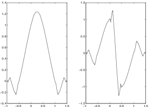
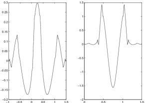
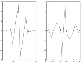
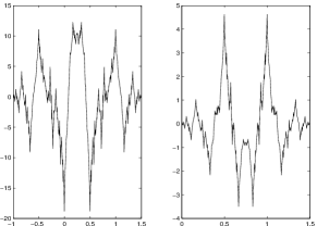
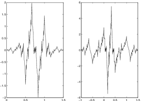
Figure 3.2: The graphs of $\eta=[\eta_{1},\eta_{2}]^{T}$, $\zeta^{1}=[\zeta^{1}_{1},\zeta^{1}_{2}]^{T}$, and $\zeta^{2}=[\zeta^{2}_{1},\zeta^{2}_{2}]^{T}$ (top, left to right), and $\widetilde{\eta}=[\widetilde{\eta}_{1},\widetilde{\eta}_{2}]^{T}$, $\widetilde{\zeta}^{1}=[\widetilde{\zeta}^{1}_{1},\widetilde{\zeta}^{1}_{2}]^{T}$, and $\widetilde{\zeta}^{2}=[\widetilde{\zeta}^{2}_{1},\widetilde{\zeta}^{2}_{2}]^{T}$ (bottom, left to right).

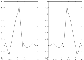
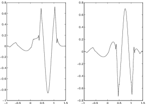
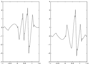
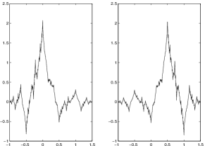
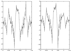
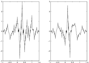
Figure 3.3: The graphs of $\phi=[\phi_{1},\phi_{2}]^{T}$, $\psi^{1}=[\psi^{1}_{1},\psi^{1}_{2}]^{T}$, and $\psi^{2}=[\psi^{2}_{1},\psi^{2}_{2}]^{T}$ (top, left to right), and $\widetilde{\phi}=[\widetilde{\phi}_{1},\widetilde{\phi}_{2}]^{T}$, $\widetilde{\psi}^{1}=[\widetilde{\psi}^{1}_{1},\widetilde{\psi}^{1}_{2}]^{T}$, and $\widetilde{\psi}^{2}=[\widetilde{\psi}^{2}_{1},\widetilde{\psi}^{2}_{2}]^{T}$ (bottom, left to right).

4 Conclusions and Remarks

In this paper, we study the matrix extension problem with symmetry for the biothogonal case. We obtain a result on representing a pair of $r\times s$ biorthogonal matrices $(\mathsf{P},\widetilde{\mathsf{P}})$ having the same compatibly symmetry and provide a step-by-step algorithm for deriving a pair of $s\times s$ biorthogonal matrices from a given pair of biorthogonal matrices $(\mathsf{P},\widetilde{\mathsf{P}})$. Our results show that for the one row case ($r=1$), the support lengths of the extension matrices can be controlled by the given pair of columns. We apply our results in this paper to the derivation of symmetric biortahogonal multiwavelets from a pair of dual $\mathsf{d}$-refinable functions.

References

- [1] Y. G. Cen and L. H. Cen, Explicit construction of compactly supported biorthogonal multiwavelets based on the matrix extension, IEEE Int. Conference Neural Networks & Signal Processing, Zhenjiang, China, June 810, 2008.
- [2] C. K. Chui and J. A. Lian, Construction of compactly supported symmetric and antisymmetric orthonormal wavelets with scale , Appl. Comput. Harmon. Anal., 2 (1995), 21–51.
- [3] L. H. Cui, Some properties and construction of multiwavelets related to different symmetric centers, Math. Comput. Simul., 70 (2005), 69–89.
- [4] L. H. Cui, A method of construction for biorthogonal multiwavelets system with multiplicity, Appl. Math. Comput., 167 (2005), 901–918.
- [5] I. Daubechies, Ten lectures on wavelets, CBMS-NSF Series in Applied Mathematics, SIAM, Philadelphia, 1992.
- [6] G. Donovan, J. Geronimo, and D. Hardin, Intertwining multiresolution analysis and the construction of piecewise-polynomial wavelets, SIAM J. Math. Anal., 27 (1996), 1791–1815.
- [7] J. Geronimo, D. P. Hardin, and P. Massopust, Fractal functions and wavelet expansions based on several scaling functions, J. Approx. Theory, 78 (1994), 373–401.
- [8] S. S. Goh and V. B. Yap, Matrix extension and biorthogonal multiwavelet construction, Lin. Alg. Appl., 269 (1998), 139–157.
- [9] B. Han, Symmetric orthonormal scaling functions and wavelets with dilation factor 4, Adv. Comput. Math., 8 (1998), 221–247.
- [10] B. Han, Approximation properties and construction of Hermite interpolants and biorthogonal multiwavelets, J. Approx. Theory, 110 (2001), 18–53.
- [11] B. Han, Matrix extension with symmetry and applications to symmetric orthonormal complex -wavelets, J. Fourier Anal. Appl., 15 (2009), 684–705.
- [12] B. Han, S. Kwon and X. S. Zhuang, Generalized interpolating refinable function vectors, J. Comput. Appl. Math., 227 (2009), 254–270.
- [13] B. Han and H. Ji, Compactly supported orthonormal complex wavelets with dilation and symmetry, Appl. Comput. Harmon. Anal., 26 (2009), 422–431.
- [14] B. Han and X. S. Zhuang, Matrix extension with symmetry and its application to filter banks, preprnt, http://arxiv.org/abs/1001.1117.
- [15] H. Ji and Z. Shen, Compactly supported (bi)orthogonal wavelets generated by interpolatory refinable functions, Adv. Comput. Math., 11 (1999), 81–104.
- [16] Q. T. Jiang, Symmetric paraunitary matrix extension and parameterization of symmetric orthogonal multifilter banks, SIAM J. Matrix Anal. Appl., 22 (2001), 138–166.
- [17] W. Lawton, S. L. Lee, and Z. Shen, An algorithm for matrix extension and wavelet construction, Math. Comp., 65 (1996), 723–737.
- [18] A. Petukhov, Construction of symmetric orthogonal bases of wavelets and tight wavelet frames with integer dilation factor, Appl. Comput. Harmon. Anal., 17 (2004), 198–210.
- [19] Z. Shen, Refinable function vectors, SIAM J. Math. Anal., 29 (1998), 235–250.
- [20] P. P. Vaidyanathan, Multirate systems and filter banks, Prentice Hall, New Jersey, 1992. (1984), 513–518.
- [21] D. C. Youla and P. F. Pickel, The Quillen-Suslin theorem and the structure of -dimesional elementary polynomial matrices, IEEE Trans. Circ. Syst., 31 (1984), 513–518.