Exchange cotunneling through quantum dots with spin-orbit coupling

Abstract

We investigate the effects of spin-orbit interaction (SOI) on the exchange cotunneling through a spinful Coulomb blockaded quantum dot. In the case of zero magnetic field, Kondo effect is shown to take place via a Kramers doublet and the SOI will merely affect the Kondo temperature. In contrast, we find that the breaking of time-reversal symmetry in a finite field has a marked influence on the effective Anderson, and Kondo models for a single level. The nonlinear conductance can now be asymmetric in bias voltage and may depend strongly on direction of the magnetic field. A measurement of the angle dependence of finite-field cotunneling spectroscopy thus provides valuable information about orbital, and spin degrees of freedom and their mutual coupling.

Quantum dots based on materials with pronounced spin-orbit interaction (SOI), such as InAs, SiGe, carbon nanotubes, and single molecules have recently received reinforced attention. Fasth07 ; Jespersen06 ; Csonka08 ; Takahashi09 ; Katsaros10 ; Kuemmeth08 ; Galpin10 ; Fang08 ; Herzog10 This is partially motivated by the quest for achieving electrical control of single spins, utilizing the fact that an electrical coupling to the orbital degrees of freedom may allow for manipulations of the spin via the SOI. Levitov03 ; Stepanenko04 ; Debald05 ; Flindt06 ; Nowack07 ; Trif07 In quantum dots, the precise form of the spin-orbit coupling depends strongly on the band structure, confining potential and dot geometry altogether. It would therefore be of great value if one could infer about the SOI directly from a measured cotunneling bias spectroscopy, which is known to produce sharp spectroscopic features due to threshold processes and/or Kondo effects.

It is well known that Kondo effect in metals with magnetic impurities like Ce and Yb, say, are strongly affected by spin-orbit interaction Coqblin69 ; Nozieres80 ; Yamada84 . The SOI modifies the spectrum of the impurity atom, but since it preserves time-reversal invariance a Kramers-degenerate groundstate remains and gives rise to Kondo effect. Likewise, a quantum dot holding a net spin-1/2, will also have its spectrum modified by SOI, and a Kramers degeneracy will still be available for Kondo effect. Unlike the atomic $\mathbf{L}\cdot\mathbf{S}$ coupling, however, the SOI in a quantum dot breaks rotational invariance and relates to specific spatial directions, akin to the effect of a crystal fields Coqblin69 ; Nozieres80 ; Yamada84 or nearby surfaces Ujsaghy98 ; Szunyogh06 in the atomic problem. Since a spinful quantum dot allows for local directional probes such as bias voltage and magnetic field, the question arises if there are effects of SOI that show up directly in a transport measurement?

Here we show that in the case where a single level approximation is valid, the SOI can be absorbed in a redefinition of the lead electron fields and thus leaves the Kondo effect unaffected. In the presence of a finite magnetic field, however, spin, and orbital contents of the Kramers doublets become disentangled and a spatial asymmetry in the tunneling amplitudes can cause the Zeeman-split Kondo peak to become asymmetric in bias voltage. This type of asymmetric splitting does not occur without SOI, unless the voltage becomes large enough to allow for real charge fluctuations on the dot. Furthermore, the SOI induced asymmetry will depend strongly on the direction of the magnetic field. The distinct angular dependence provides a very direct signature of the SOI in a quantum dot, thus providing valuable information about the quantum dot in question.

We employ the following general single-particle Hamiltonian to describe a quantum dot defined by a potential $V(\mathbf{r})$ and placed in an external magnetic field

$$\mathcal{H}_{d}= \frac{({\mathbf{p}}\!-\!e{\mathbf{A}})^{2}}{2m}+V({\mathbf{r}})+g\mu_{B}{\mathbf{B}}\cdot{\boldsymbol{\tau}}$$

$$\hskip 28.45274pt+\frac{e\hbar}{4m^{2}c^{2}}[\mathbf{{E}(r)\times(\mathbf{p}-e\mathbf{A})]\cdot{\boldsymbol{\tau}},}$$ (1)

with ${\boldsymbol{\tau}}$ denoting the vector of Pauli matrices, and $\mathbf{B}$ the external magnetic field corresponding to a vector potential $\mathbf{A}$. The spin-orbit coupling is here kept on its most generic form in terms of the relevant nuclear or structural electrical field $\mathbf{E}({\mathbf{r}})$. The potential contains both the periodic potential from the ionic background and the imposed confining potentials defining the dot.

In the absence of an external field $({\mathbf{A}}={\mathbf{0}})$, this Hamiltonian is symmetric under time reversal and its eigenstates therefore take the form of Kramers doublets of two spinors Sakurai94 :

$$\psi_{n\Uparrow}(\mathbf{{r})=\left(\begin{array}[]{c}u_{n}({r})\\ v_{n}({r})\end{array}\right),\,\,\,\,\psi_{n\Downarrow}({r})=\left(\begin{array}[]{c}-v_{n}^{\ast}({r})\\ u_{n}^{\ast}({r})\end{array}\right),}$$ (2)

where the wavefunction components $u_{n}$ and $v_{n}$ depend strongly on the confining potential. The corresponding eigenenergies, $\varepsilon_{n}$, come with a characteristic level spacing set by the confining potential and the strength of the SOI. Also the source, and drain electrodes may experience a SOI, so in general, we can express the eigenstates of the corresponding Hamiltonian in the leads, $\mathcal{H}_{L/R}$, in the same way:

$$\psi_{\alpha\mathbf{k}\uparrow}(\mathbf{{r})=}\left(\begin{array}[]{c}a_{\alpha\mathbf{k}}(\mathbf{r})\\ b_{\alpha\mathbf{k}}(\mathbf{r})\end{array}\right)\mathbf{,\,\,\,\,}\psi\mathbf{{}_{\alpha\mathbf{k}\downarrow}({r})=}\left(\begin{array}[]{c}-b_{\alpha\mathbf{k}}^{\ast}(\mathbf{r})\\ a_{\alpha\mathbf{k}}^{\ast}(\mathbf{r})\end{array}\right),$$ (3)

where $\alpha=L,R$ refers to left, and right lead, respectively. Using these eigenstates, the total many-body Hamiltonian is given by

$$H= \sum_{\overset{\alpha=L/R}{\mathbf{k},\,\nu}}(\varepsilon_{k}-\mu_{\alpha})c_{\alpha\mathbf{k}\nu}^{\dagger}c_{\alpha\mathbf{k}\nu}+\sum_{n,\eta}\varepsilon_{n}d_{n\eta}^{\dagger}d_{n\eta}$$ (4)

$$+\sum_{\overset{\alpha=L/R}{\mathbf{k},\,\nu,\,\eta,n}}\left(t^{\nu\eta}_{\alpha kn}c_{\alpha\mathbf{k}\nu}^{\dagger}d_{n\eta}+t^{\eta\nu}_{n\alpha k}d_{n\eta}^{\dagger}c_{\alpha\mathbf{k}\nu}\right)+H_{int},$$

where $c_{\alpha k\nu}^{\dagger}$ creates an electron in the $\nu$’th component of the Kramers doublet $(\nu=\uparrow/\downarrow)$ with momentum $\mathbf{k}$ in lead $\alpha=L/R$, and $d_{n\eta}^{\dagger}$ creates an electron in the $\eta$’th component $(\eta=\Uparrow/\Downarrow)$ of the $n$’th Kramers doublet on the dot. For the interaction term we employ the constant interaction model $H_{int}=E_{C}(N-N_{g})^{2}$, where $E_{C}$ denotes the total capacitive charging energy of the dot.

The amplitudes for tunneling between dot and leads $t^{\alpha kn}_{\nu\eta}$ depend on the index of the Kramers doublets and it is given by the Hamiltonian overlap,

$$t^{\alpha\mathbf{k}n}_{\nu\eta}=\int\!\!d{\mathbf{r}}\,\,\psi^{\ast}_{\alpha\mathbf{k}\nu}(\mathbf{r})\mathcal{H}_{tot}(\mathbf{r})\psi_{n\eta}(\mathbf{r}),$$ (5)

where the total single-particle Hamiltonian still takes the form of Eq. (1), but with an extended potential defining two tunneling barriers which support the distinction into leads and dot ($\mathcal{H}_{tot}=\mathcal{H}_{d}+\mathcal{H}_{L}+\mathcal{H}_{R}$) made in our definition of the eigenfunctions for the separate parts. Regardless of the details of this potential, this first-quantized Hamiltonian takes the following form:

$$\mathcal{H}_{tot}(\mathbf{r})=\mathcal{H}_{0}(\mathbf{r})\tau^{0}+i\lambda_{so}\varepsilon_{ijk}\tau^{i}E_{j}(\mathbf{r})\partial_{x_{k}},$$ (6)

with kinetic energy and local potential contained in $\mathcal{H}_{0}(\mathbf{r})$ and the local spin-orbit term written in terms of the Levi-Cevita symbol $\varepsilon_{ijk}$ (Einstein summation convention implied). Using the fact that the different Kramers doublet components can be related via time reversal Sakurai94 , i.e.

$$\psi_{n\Uparrow,\sigma}=i\tau^{y}_{\sigma\sigma^{\prime}}\psi^{\ast}_{n\Downarrow,\sigma^{\prime}},$$ (7)

together with the relation $\tau^{y}\tau^{i}\tau^{y}=-(\tau^{i})^{\ast}$, it is readily demonstrated that

$$\langle\alpha\mathbf{k}\downarrow|\mathcal{H}_{tot}|n\Downarrow\rangle= \,\langle\alpha\mathbf{k}\uparrow|\mathcal{H}_{tot}|n\Uparrow\rangle^{\ast},$$ (8)

$$\langle\alpha\mathbf{k}\downarrow|\mathcal{H}_{tot}|n\Uparrow\rangle= -\langle\alpha\mathbf{k}\uparrow|\mathcal{H}_{tot}|n\Downarrow\rangle^{\ast},$$ (9)

which renders the tunneling amplitude proportional to a unitary matrix in $\nu\eta$ space:

$$t^{\alpha\mathbf{k}n}_{\nu\eta}=t_{\alpha\mathbf{k}n}\mathbb{U}^{\alpha{\mathbf{k}n}}_{\nu\eta}.$$ (10)

Next, we consider a specific charge state with an odd number of electrons on the dot and assume all levels below the $m$’th level to be doubly occupied. For the singly occupied $m$’th level the dimensionless unitary matrix in Eq. (10) can be now be absorbed in a redefinition of the fermion fields in the two leads: ${\tilde{c}}^{\dagger}_{\alpha\mathbf{k}\eta}=c^{\dagger}_{\alpha\mathbf{k}\nu}\mathbb{U}^{\alpha{\mathbf{k}m}}_{\nu\eta}$. For sufficiently large level spacings, we thus end up with the following single-orbital Anderson model:

$$H= \sum_{\alpha\mathbf{k}\eta}(\varepsilon_{k}-\mu_{\alpha}){\tilde{c}}^{\dagger}_{\alpha\mathbf{k}\eta}{\tilde{c}}_{\alpha\mathbf{k}\eta}+\sum_{\eta}\varepsilon_{m}d_{m\eta}^{\dagger}d_{m\eta}$$

$$+\sum_{\alpha\mathbf{k}\eta}t_{\alpha\mathbf{k}m}\left({\tilde{c}}_{\alpha\mathbf{k}\eta}^{\dagger}d_{m\eta}+d_{m\eta}^{\dagger}{\tilde{c}}_{\alpha\mathbf{k}\eta}\right)+H_{int},$$ (11)

which no longer bears any trace of the SOI. Notice that this unitary transformation is specific to the $m$’th level and therefore tunneling amplitudes to any of the other levels on the dot will in general retain their full (unitary) $2\times 2$ matrix structure in $\nu\eta$ space. Apart from its influence on the precise magnitude of $t_{\alpha\mathbf{k}m}$, SOI thus appears to have no effect whatsoever on transport phenomena involving only a single level. In particular, the Kramers degeneracy of this level will give rise to Kondo effect.

This conclusion changes dramatically in the case of a finite applied magnetic field, which couples directly to the constituent quantum numbers of the Kramers doublets, i.e. to spin, and orbital degrees of freedom. Using symmetric gauge, ${\bf A}({\bf r})=({\bf B}\times{\bf r})/2$, the magnetic field enters $\mathcal{H}_{d}$ through the kinematic momentum. This gives rise to the following first quantized terms:

$$\mathcal{H}_{B}= -\mu_{B}{\bf B}\cdot{\bf L}+\mu_{B}\frac{e}{4}(r^{2}B^{2}-({\bf r}\cdot{\bf B})^{2})$$ (12)

$$+\mu_{B}\left[g{\bf B}+\left(({\bf E}({\bf r})\cdot{\bf B}){\bf r}-({\bf E}({\bf r})\cdot{\bf r}){\bf B}\right)\frac{e}{4mc^{2}}\right]\cdot{\boldsymbol{\tau}},$$

with an orbital term depending on the angular momentum operator ${\bf L}$, a diamagnetic term quadratic in $B$, and a local anisotropic Zeeman term. The terms linear in $B$ both break the time-reversal symmetry and thus destroy the degeneracy of the Kramers doublets. We shall assume $B$ to be weak enough that this splitting, which we parameterize by an effective $g$ factor, ${\tilde{g}}$, is much smaller than the relevant zero-field level spacing, i.e. ${\tilde{g}}\mu_{B}B\ll\Delta\varepsilon\equiv\min[\varepsilon_{m+1}-\varepsilon_{m},\varepsilon_{m}-\varepsilon_{m-1}]$.

Apart from this renormalization of the Zeeman splitting within the $m$’th level, the linear terms in $B$ also have off-diagonal terms which couple the state $|m\eta\rangle$ to other states $|n\eta^{\prime}\rangle$ via ${\bf L}$ and ${\boldsymbol{\tau}}$. The amplitudes for tunneling into the resulting finite $B$ eigenstates of the dot are therefore changed and in particular the unitarity of $t_{\alpha{\bf k}m}^{\eta^{\prime}\!\eta}$ used for $B=0$ is no longer guaranteed. In general, the matrix of tunneling amplitudes can be polar decomposed into a product of a unitary and a hermitian matrix. The unitary part can again be absorbed in a canonical transformation of the conduction electrons in the corresponding lead and $t_{\alpha{\bf k}m}^{\eta^{\prime}\!\eta}$ can be taken to be hermitian in $\eta^{\prime}\!\eta$ space. Altogether, the tunneling term in (11) is therefore modified to

$$H_{T}= \sum_{\alpha{\bf k}\eta^{\prime}\!\eta}\left(t_{\alpha{\bf k}m}^{\eta^{\prime}\!\eta}{\tilde{c}}_{\alpha{\bf k}\eta^{\prime}}^{\dagger}\tilde{d}_{m\eta}+(t_{\alpha{\bf k}m}^{\eta^{\prime}\eta})^{\!\ast}\tilde{d}_{m\eta}^{\dagger}{\tilde{c}}_{\alpha{\bf k}\eta^{\prime}}\right),$$ (13)

where electron creation operators, $\tilde{d}_{m\eta}^{\dagger}$ and ${\tilde{c}}_{\alpha{\bf k}\eta^{\prime}}^{\dagger}$, as well as tunneling amplitudes $t_{\alpha{\bf k}m}^{\eta^{\prime}\!\eta}$ now depend on the applied magnetic field.

Kondo model: Within the Kondo regime, $\max(\nu_{F,\alpha}|(t_{\alpha^{\prime}m}^{\eta\eta^{\prime}})^{\ast}t_{\alpha m}^{\eta^{\prime\prime}\eta^{\prime\prime\prime}}|)\ll\min(-\varepsilon_{m},\varepsilon_{m}+E_{C})$, a Schrieffer-Wolff transformation Schrieffer66 with the full $\eta^{\prime}\eta$ matrix tunneling amplitudes now leads to the following exchange-cotunneling (Kondo) model:

$$H_{K}= \sum_{\alpha{\bf k}\eta}(\varepsilon_{k}-\mu_{\alpha}){\tilde{c}}^{\dagger}_{\alpha{\bf k}\eta}{\tilde{c}}_{\alpha{\bf k}\eta}+\mu_{B}{\tilde{g}}^{ij}B^{i}S^{j}$$ (14)

$$\hskip 28.45274pt+\frac{1}{2}\sum_{\stackrel{{\scriptstyle\alpha^{\prime}\alpha,{\bf k^{\prime}}{\bf k},\eta^{\prime}\eta}}{{i,j=0,x,y,z}}}J^{ij}_{\alpha^{\prime}\alpha}S^{i}\,{\tilde{c}}^{\dagger}_{\alpha^{\prime}{\bf k}^{\prime}\eta^{\prime}}\tau^{j}_{\eta^{\prime}\eta}{\tilde{c}}_{\alpha{\bf k}\eta},$$

with $S^{0}=\mathds{1}$, $\tau^{0}_{\eta^{\prime}\eta}=\delta_{\eta^{\prime}\eta}$ and cotunneling amplitudes:

$$J^{ij}_{\alpha^{\prime}\alpha}={\rm Tr}[t_{\alpha^{\prime}m}\tau^{i}t_{\alpha m}^{\dagger}\tau^{j}]\frac{\varepsilon_{+}+(-1)^{\delta_{i0}}\varepsilon_{-}}{2^{(\delta_{i0}+\delta_{j0})}\varepsilon_{+}\varepsilon_{-}},$$ (15)

where $\varepsilon_{\pm}$ denotes the addition, and subtraction energies on the dot. Away from the particle-hole symmetric point, $\varepsilon_{+}=\varepsilon_{-}$, a vector of potential scattering amplitudes, $J^{0j}$, is present. Notice also that expanding (15) to leading order in $B$, it follows from the hermiticity of $t_{\alpha{\bf k}m}^{\eta^{\prime}\!\eta}$ that the intra-lead exchange couplings will be diagonal and isotropic, i.e. $J^{ij}_{\alpha^{\prime}\alpha}\propto\delta_{ij}$.

It is interesting to note that this exchange scattering has lead indices ($L/R$) mixed up with Kramers doublet indices ($\eta$) in such a way that the usual simplification to a single channel Kondo model no longer is possible. For $B=0$ (or without SOI) only one channel is involved, but a finite field breaks the L/R symmetry via the SOI and gives rise to a channel asymmetric two-channel (anisotropic) Kondo model. As we shall demonstrate below, certain system geometries will have zero Zeeman splitting in finite magnetic field and therefore a strong coupling two-channel regime Rosch01 ; Pustilnik04 should in fact be attainable for such geometries.

Cotunneling current: From these cotunneling amplitudes one can now calculate the current through the dot as Bruus04 $I=e\sum_{\eta^{\prime}\eta}(\Gamma^{RL}_{\eta^{\prime}\eta}-\Gamma^{LR}_{\eta^{\prime}\eta})P(\eta)$, The non-equilibrium occupation numbers $P(\eta)$ for the dot states satisfy a rate equation from which they are found to be $P(\eta)=\Gamma_{\eta\bar{\eta}}/(\Gamma_{\eta\bar{\eta}}+\Gamma_{\bar{\eta}\eta})$, with $\Gamma_{\eta^{\prime}\eta}=\sum_{\alpha^{\prime}\alpha}\Gamma^{\alpha^{\prime}\alpha}_{\eta^{\prime}\eta}$. These cotunneling rates are found as $\Gamma^{\alpha^{\prime}\alpha}_{\eta^{\prime}\eta}=\gamma^{\alpha^{\prime}\alpha}_{\eta^{\prime}\eta}\Delta\varepsilon^{\alpha^{\prime}\alpha}_{\eta^{\prime}\eta}n_{B}(\Delta\varepsilon^{\alpha^{\prime}\alpha}_{\eta^{\prime}\eta})$ where $n_{B}$ is the Bose function and the energy differences are defined as $\Delta\varepsilon^{\alpha^{\prime}\alpha}_{\eta^{\prime}\eta}=\tilde{\varepsilon}_{m,\eta^{\prime}}-\tilde{\varepsilon}_{m,\eta}-\mu_{\alpha}+\mu_{\alpha^{\prime}}$. Finally, the tunneling probabilities are $\gamma^{\alpha^{\prime}\alpha}_{\eta^{\prime}\eta}=\pi\nu_{F,\alpha^{\prime}}\nu_{F,\alpha}\sum_{ijk}J^{ij}_{\alpha^{\prime}\alpha}J^{ik}_{\alpha\alpha^{\prime}}\tau^{j}_{\eta^{\prime}\eta}\tau^{k}_{\eta\eta^{\prime}}$. Notice that this is a real number since $(J^{ij}_{\alpha^{\prime}\alpha})^{\ast}=J^{ij}_{\alpha\alpha^{\prime}}$. As for a system without SOI, the nonlinear conductance will exhibit cusped steps at bias voltage, $V=\mu_{L}-\mu_{R}$, corresponding to the effective Zeeman splitting. Since, however, Kramers doublet and lead indices are mixed for finite magnetic field, the nonlinear conductance is no longer symmetric in bias voltage. In general, the two cusps at respectively positive and negative bias can now be of different magnitude, and their relative magnitude will in general depend on the angle of the magnetic field.

Two-level model: To better illustrate these results, we now exemplify our discussion by a simple two-level model (cf. Fig. 1). With two levels split by an energy $\delta$, we can express the Hamiltonian in the basis $\{|1\uparrow\rangle$, $|1\downarrow\rangle$, $|2\uparrow\rangle$, $|2\downarrow\rangle\}$, where the wave functions of the two levels, $\psi_{1}$ and $\psi_{2}$, are chosen to be real. In this basis, the spin-orbit coupling is included to give the full dot Hamiltonian:

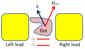
Figure 1: Sketch of two-orbital model system characterized by spin-orbit field $\mathbf{B}_{SO}$ and the angular momentum vector $\boldsymbol{\lambda}$.

$$\langle i\sigma|H_{0}|j\sigma^{\prime}\rangle=-\tau^{z}_{ij}\tau^{0}_{\sigma\sigma^{\prime}}\delta/2+\tau^{y}_{ij}\tau^{z}_{\sigma\sigma^{\prime}}\Delta_{SO}/2,$$ (16)

where we have chosen the spin quantization along the built-in spin-orbit field, $\mu_{B}\mathbf{B}_{SO}=\frac{e\hbar}{2mc^{2}}\langle\psi_{1}|\mathbf{E}(\mathbf{r})\times\mathbf{p}|\psi_{2}\rangle\equiv-\mathbf{\hat{z}~{}}i\Delta_{SO}/2$, characteristic for these two levels. $H_{0}$ is diagonalized by two Kramers doublets:

$$|a\eta\rangle = u|1\eta\rangle-iv\tau^{z}_{\eta\eta}|2\eta\rangle,$$ (17a)

$$|b\eta\rangle = v|1\eta\rangle+iu\tau^{z}_{\eta\eta}|2\eta\rangle,$$ (17b)

with $u^{2}+v^{2}=1$, $2uv=\Delta_{SO}/\Delta$, $\Delta=\sqrt{\delta^{2}+\Delta_{SO}^{2}}$ and eigenenergies $E_{a/b}=\mp\Delta/2$. Note that these doublets follow the general structure of time-reversed pairs in Eq. (2). In the presence of a magnetic field, we shall neglect the quadratic term in (12) altogether. This amounts to assuming the dot to be much smaller than the magnetic length, i.e. $eB\ell_{dot}^{2}\ll\hbar$, which will then ensure that $eB^{2}\langle r^{2}\rangle-e\langle({\bf r}\cdot{\bf B})^{2}\rangle\ll\langle({\bf r}\times{\bf p})\cdot{\bf B}\rangle$. The remaining linear terms in Eq. (12) have the following matrix elements in the original four-state basis:

$$\langle i\sigma|H_{B}|j\sigma^{\prime}\rangle=\frac{g_{0}\mu_{B}}{2}\tau^{0}_{ij}\mathbf{B}\cdot\boldsymbol{\tau}_{\sigma\sigma^{\prime}}+i\mu_{B}\tau^{y}_{ij}\tau^{0}_{\sigma\sigma^{\prime}}\boldsymbol{\lambda}\cdot\mathbf{B},$$ (18)

where $\boldsymbol{\lambda}=-i\langle 1|\mathbf{L}|2\rangle$ is a (real) vector characteristic for the two levels. Expressing this in the zero-field eigenbasis ($a,b$ doublets), we can now find the low field splitting of the individual doublets. That is, for fields low enough that this splitting will be much smaller than $\Delta$, we obtain the effective single-doublet ($m=a,b$) Hamiltonians:

$$\langle m\eta|H_{B}|m\eta^{\prime}\rangle=\frac{g_{0}\mu_{B}}{2}BZ_{m}(\sin\xi_{m},0,\cos\xi_{m})\cdot\boldsymbol{\tau}_{\eta\eta^{\prime}}$$ (19)

where we have defined

$$Z_{a/b}=\sqrt{\frac{\delta^{2}\sin^{2}\zeta}{\delta^{2}+\Delta_{SO}^{2}}+\left(\cos\zeta\pm\frac{2\tilde{\lambda}\Delta_{SO}}{g_{0}\Delta}\right)^{2}},$$ (20)

with $\sin\xi_{a/b}=\pm\delta(\sin\zeta)/(Z_{a/b}\Delta)$ and where $\tilde{\lambda}=|\boldsymbol{\lambda}|(\cos\zeta\cos\theta+\sin\zeta\cos\varphi\sin\theta)$ denotes the projection of $\boldsymbol{\lambda}$ on $\mathbf{B}$ in terms of the relative angles $(\zeta,\theta,\varphi$) between the two intrinsic vectors, $\mathbf{B}_{SO}$ and $\boldsymbol{\lambda}$, and the external $\mathbf{B}$, all indicated in Fig. 2(a). The eigenstates of this hamiltonian are readily found by a rotation within the plane spanned by $\mathbf{B}_{SO}$ and $\mathbf{B}$, i.e. $|\widetilde{m\eta}\rangle^{(0)}=\mathbb{R}_{y}(\xi_{m})|m\eta\rangle$, where $\mathbb{R}_{y}(\xi)=\tau^{0}\cos(\xi/2)+i\tau^{2}\sin(\xi/2)$. Apart from this splitting, a finite field will also mix the $a$ and $b$ doublets. Starting from this last eigenbasis, which only refers to the direction of $\mathbf{B}$, we include this mixing to linear order in the magnitude $|\mathbf{B}|$ from first order perturbation theory, i.e. $|\widetilde{a\eta}\rangle^{(1)}=|\widetilde{a\eta}\rangle^{(0)}+\langle b\eta^{\prime}|H_{B}|a\eta^{\prime\prime}\rangle[\mathbb{R}_{y}(\xi_{a})]_{\eta\eta^{\prime\prime}}|b\eta^{\prime}\rangle^{(0)}$, where $\langle b\eta^{\prime}|H_{B}|a\eta\rangle=(\tilde{\lambda}\delta\tau^{z}_{\eta^{\prime}\eta}-g_{0}\sin(\zeta)\Delta_{SO}\tau^{x}_{\eta^{\prime}\eta}/2)\mu_{B}B/\Delta$. The amplitudes for tunneling into this lowest lying Zeeman-split Kramers doublet $|\widetilde{a\eta}\rangle^{(1)}$, are now readily found using (17). Notice that it is only this last non-unitary mixing of $a$ and $b$ doublets which prevents us from diagonalizing $t_{\alpha a}^{\eta\eta^{\prime}}$ by a canonical transformation of the conduction electrons.

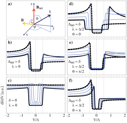
Figure 2: (a) Geometry of vectors $\boldsymbol{\lambda}$, $\mathbf{B}_{SO}$, and $\mathbf{B}$, indicating their relative angles. $\mathbf{B}_{SO}$ and $\mathbf{B}$ span the $x-z$ plane. (b-f) Nonlinear conductance, $dI/dV$, in arbitrary units vs. bias voltage in units of $\Delta$ for a set of representative parameters given in the insets. Each panel shows a progression of curves with varying $\zeta$, moving from the thick solid (black) curve with $\zeta=0$ to the thick dashed (black) curve with $\zeta=\pi/2$. Remaining parameters are $g\mu_{B}B=0.5\Delta$, $\varphi=\pi/4$, $t_{1,L/R}=1$, $t_{2,L}=3$, $t_{2,R}=0.1$. Notice the closing of the Zeeman splitting for $\mathbf{B}\perp\mathbf{B}_{SO}$ for two solely SOI-split orbitals in panel (c). This can also be seen analytically from Eq. (20).

Whereas the SOI could not be discerned at zero field, the angle-dependent bias voltage asymmetry of $dI/dV$, confirmed by our simple model in Figs. 2(b-f), is a unique signature of SOI at finite field. Such bias asymmetries have often been found in experiments on various quantum dots. Jespersen06 ; Schmauss09 Nevertheless, it is often difficult to rule out the influence of incipient charge fluctuations, setting in at slightly higher bias voltages, as the source of this asymmetry. The only unambiguous evidence for such SOI-induced bias asymmetry will therefore be the observation of its variation with a change in the direction of the magnetic field. Taken together with the possible angle dependence of the Zeeman splitting itself (cf. e.g. Refs. Takahashi09, ; Katsaros10, ), such a measurement can thus reveal otherwise inaccessible details on the spin-orbit coupling in a given quantum dot.

We thank V. Golovach and P. Brouwer for stimulating discussions and acknowledge financial support from the Danish Agency for Science, Technology and Innovation and from the European Union under the FP7 STREP program SINGLE (J.P., K.F.).

References

• (1) C.ย Fasth et al., Phys. Rev. Lett. 98, 266801 (2007).
• (2) T.ย S.ย Jespersen et al., Phys. Rev. B 74, 233304 (2006).
• (3) S.ย Csonka et al., Nano Lett. 8, 3932 (2008).
• (4) S.ย Takahashi et al., arXiv:0912.3088v1.
• (5) G.ย Katsaros et al., Nat. Nanotech. (2 May 2010) doi:10.1038/nnano.2010.84 Article
• (6) F.ย Kuemmeth, S.ย Ilani, D.ย Ralph, and P.ย McEuen, Nature, 452, 448-452 (2008).
• (7) M.ย R.ย Galpin et al., Phys. Rev. B 81, 075437 (2010).
• (8) T.-F.ย Fang, w.ย Zuo, and H.-G.ย Luo, Phys. Rev. Lett. 101, 246805 (2008).
• (9) S. Herzog, M. R. Wegewijs, arXiv:0911.0571.
• (10) L.ย S.ย Levitov and E.ย I.ย Rashba, Phys. Rev. B 67, 115324 (2003).
• (11) D.ย Stepanenko and N.ย E.ย Bonesteel, Phys. Rev. Lett. 93, 140501 (2004).
• (12) S.ย Debald and C.ย Emary, Phys. Rev. Lett. 94, 226803 (2005).
• (13) C.ย Flindt, A.ย S.ย Sรธrensen, and K.ย Flensberg, Phys. Rev. Lett. 97, 240501 (2006).
• (14) K.ย C.ย Nowack et al., Science 318, 1430 (2007).
• (15) M.ย Trif, V.ย N.ย Golovach, and D.ย Loss, Phys. Rev. B 75, 085307 (2007).
• (16) B.ย Coqblin, and J.ย R.ย Schrieffer, Phys. Rev. 185, 847 (1969).
• (17) P.ย Noziรจres, and A.ย Blandin, J. Phys. 41, 193 (1980).
• (18) K.ย Yamada, K.ย Yosida, and K.ย Hanzawa, Prog. Theor. Phys. 71, 450 (1984).
• (19) O.ย รšjsรกghy, and A.ย Zawadowski, Phys. Rev. B 57, 11598 (1998).
• (20) L.ย Szunyogh et al., Phys. Rev. Lett. 96, 067204 (2006).
• (21) Cf. e.g. Ch. 4.4 in J.ย J.ย Sakurai, Modern Quantum Mechanics (Addison-Wesley Publishing Company, 1994).
• (22) J.ย R.ย Schrieffer, and P.ย A.ย Wolff, Phys. Rev. 149, 491 (1966).
• (23) A.ย Rosch, J.ย Kroha, and P.ย Wรถlfle, Phys. Rev. Lett. 87, 156802 (2001).
• (24) M.ย Pustilnik, L.ย Borda, L.ย I.ย Glazman, and J.ย von Delft, Phys. Rev. B 69, 115316 (2004).
• (25) H.ย Bruus and K.ย Flensberg, Many-body Quantum Theory in Condensed Matter Physics (Oxford University Press, Oxford, 2004).
• (26) S. Schmaus et al., Phys. Rev. B 79, 045105 (2009).