Meir-Wingreen formula for heat transport in a spin-boson nanojunction model

Abstract

An analog of the Meir-Wingreen formula for the steady-state heat current through a model molecular junction is derived. The expression relates the heat current to correlation functions of operators acting only on the degrees of freedom of the molecular junction. As a result, the macroscopic heat reservoirs are not treated explicitly. This allows one to exploit methods based on a reduced description of the dynamics of a relatively small part of the overall system to evaluate the heat current through a molecular junction. The derived expression is applied to calculate the steady-state heat current in the weak coupling limit, where Redfield theory is used to describe the reduced dynamics of the molecular junction. The results are compared with those of previously developed approximate and numerically exact methods.

I Introduction

Heat transport in nanoscale molecular junctions, i.e., in molecules that interconnect metal or semiconductor electrodes, is a process that is crucial for the stability of the junction and thus for potential molecular electronic devices.Montgomery2002-5377 ; Chen2003-1691 ; Segal2003-6840 ; Huang2006-1240 ; Pecchia2007-035401 ; Ioffe2008-727 ; Hartle2009-146801 It has been demonstrated experimentally that the localized Joule heating may induce a substantial temperature increase within a molecule-metal contact due to inefficient heat dissipation.Huang2006-1240 Theoretical studies of heat transport at the nanoscale, in particular the dependence of heat dissipation on various physical parameters of a molecular junction, will thus provide valuable insight into the transport mechanisms thus facilitating the interpretation of experimental results and the design of novel nanoscale electronic devices.

Segal and Nitzan investigated the characteristics of heat transport of a spin-boson nanojunction model (SBNM), where a two-level system is simultaneously connected to two heat reservoirs (baths) of different temperatures.Segal2005-034301 ; Segal2005-194704 ; Segal2006-026109 Based on these studies, they suggested possible realization of novel nano-devices such as a thermal rectifierSegal2005-034301 ; Segal2005-194704 and a molecular heat pump.Segal2006-026109 The methodology used in their work assumes weak coupling between the two-level system and the reservoirs so that Redfield theoryRedfield1957-19 ; Redfield1965-1 may be applied. This assumption may not always hold for a realistic molecular junction where the energy flow may be enhanced/maximized by tuning certain physical parameters. To address this problem, we have developed a numerically exact methodologyVelizhanin2008-325 to study the dynamics of the SBNM. The methodology is based on the multilayer multiconfiguration time-dependent Hartree (ML-MCTDH) theory,Wang2003-1289 which is a non-perturbative and numerically exact approach. Thus, it can provide accurate results in a broader range of physical regimes (within the model). For example, our previous study has revealed a turnover behavior of the heat current with respect to the coupling strength between the two-level system and the heat baths. As a consequence, the optimization of heat transport is possible by choosing an appropriate set of physical parameters.

Numerically exact simulationsVelizhanin2008-325 also provide benchmark results that can be used to develop more accurate approximate theories. This is the focus of the present paper. From a broader perspective, the spin-boson nanojunction model is a two-bath, nonequilibrium version of the standard spin-boson Hamiltonian for studying electron transfer reactions.Leggett1987-1 ; Weiss1999 To date, the reduced dynamics of the two-level system has been of primary interest and various approximate approaches have been developed to study this dynamics. Examples include the noninteracting blip approximation,Leggett1987-1 ; Aslangul1986-1657 Redfield theory,Redfield1957-19 ; Redfield1965-1 Zusman equationZusman1980-295 and its generalization to the low temperature domain.Ankerhold2004-1436 It is desirable to apply these methods directly to the study of heat transport in the spin-boson nanojunction model. However, this is not straightforward since the operator for heat current involves not only the degrees of freedom of the two-level system but also those of the heat baths.

On the other hand, the relation between the reduced dynamics of an open system and the current flowing through it was found in the theory of electron transport in mesoscopic systems by Meir and Wingreen.Meir1992-2512 They derived a Landauer-type expression that relates the electrical current to certain correlation functions of the small mesoscopic system. The goal of this paper is to derive a similar expression for the heat current through a two-level system, driven out of equilibrium by two heat baths. Based on the thus obtained expression, the approximate methods mentioned above can be used to study heat transport properties of the SBNM.

The remainder of the paper is organized as follows. The model Hamiltonian and the observable of interest are described in Sec. II.1. Section II.2 describes the theoretical techniques that allow us to express the heat current through correlation functions of the two-level system. The final Meir-Wingreen type expression for the steady-state heat current is obtained in Section II.3. As a demonstration, we apply the developed theory in Sec. II.4 to evaluate the heat current in the limit of weak coupling between the two-level system and the baths. In Sec. III this heat current is compared with the results obtained using the Segal-Nitzan approach and the numerically exact simulations. Sec IV concludes.

II Theory

II.1 Spin-Boson nanojunction model

The spin-boson nanojunction model (SBNM) considered in this work Segal2005-034301 ; Segal2005-194704 ; Segal2006-026109 ; Velizhanin2008-325 consists of two heat reservoirs (baths) interconnected by a bridge, which is represented by a two-level system (TLS) (see Fig. 1).

Figure 1: Spin-Boson nanojunction model.

The heat baths at different temperatures drive the TLS out of equilibrium and the dependence of the heat current through the TLS on various parameters of the model can be studied. The SBNM Hamiltonian reads as

$$H=H_{B}+H_{S}+H_{SB},$$ (1)

where $H_{B}$ describes the two harmonic baths, “cold” ($C$) and “hot” ($H$) (atomic units are assumed throughout the paper)

$$H_{B}=H_{C}+H_{H},$$

$$H_{K}=\sum_{m\in K}\omega_{m}a^{\dagger}_{m}a_{m};~{}~{}K=C,H,$$ (2)

where $a^{\dagger}_{m}$ ($a_{m}$) are bosonic creation (annihilation) operators. The bridge Hamiltonian $H_{S}$ in the second quantization reads

$$H_{S}=\sum_{i=1,2}E_{i}n_{ii};~{}~{}E_{2}-E_{1}=\epsilon>0,$$ (3)

where $n_{ij}\equiv c^{\dagger}_{i}c_{j}$ and $c^{\dagger}_{i}$ ($c_{j}$) is a fermionic creation (annihilation) operator. The energy spacing between the two levels of the bridge is denoted by $\epsilon$. The coupling between the bath and the TLS is given by

$$H_{SB}=H_{SC}+H_{SH},$$

$$H_{SK}=\sum_{m\in K}V_{m}(a^{\dagger}_{m}+a_{m})[n_{21}+n_{12}];~{}~{}K=C,H.$$ (4)

The dynamics of the TLS is restricted to the single-particle space spanned by the basis functions $|1\rangle=c^{\dagger}_{1}|{\rm vac}\rangle$ and $|2\rangle=c^{\dagger}_{2}|{\rm vac}\rangle$, where $|{\rm vac}\rangle$ denotes the fermionic vacuum. This restriction guarantees that the TLS representation by Hamiltonian (3) is equivalent to the more commonly used form,Leggett1987-1 ; Weiss1999 $H_{S}=\frac{\epsilon}{2}(|2\rangle\langle 2|-|1\rangle\langle 1|)$. On the other hand, the fermionic representation introduced here is more convenient for the diagrammatic technique exploited in Sec. II.2.

Starting with the Heisenberg operator of the heat current from the TLS to the cold bath

$$I_{C}(t)\equiv i[H,H_{C}](t)=i\left[H,\sum_{m\in C}\omega_{m}a^{\dagger}_{m}a_{m}\right](t),$$ (5)

straightforward algebra gives the expectation value of the heat current

$$\langle I_{C}(t)\rangle=-2{\rm Im}\left[\sum_{i,j;~{}m\in C}\omega_{m}V^{ij}_{m}M^{>}_{m,ij}(t,t)\right].$$ (6)

In this expression we introduce the notation

$$V^{ij}_{m}=(1-\delta_{ij})V_{m},$$ (7)

and the nonequilibrium Green’s function (NEGF) $M_{m,ij}(t,t^{\prime})$ defined on the Schwinger-Keldysh contourSchwinger1961-407 ; Keldysh1965-1018 (depicted in Fig. 2)

$$M_{m,ij}(t,t^{\prime})=\langle T_{c}[a_{m}(t)n_{ij}(t^{\prime})]\rangle$$ (8a)

$$M_{m,ij}(t,t^{\prime})=\left\{\begin{array}[]{ll}M^{>}_{m,ij}(t,t^{\prime});~{}~{}t>_{c}t^{\prime},\\ M^{<}_{m,ij}(t,t^{\prime});~{}~{}t<_{c}t^{\prime},\\ \end{array}\right.$$ (8b)

where $t>_{c}t^{\prime}$ means that $t$ is ”later” on the contour than $t^{\prime}$ as is illustrated in Fig. 2.

Figure 2: The Schwinger-Keldysh contour.

The contour-ordering operator $T_{c}$ moves operators with later (in the contour sense) time-arguments to the left. Thus, in accordance with Eq. (8), the greater and the lesser Green’s functions are defined as $M^{>}_{m,ij}(t,t^{\prime})=\langle a_{m}(t)n_{ij}(t^{\prime})\rangle$ and $M^{<}_{m,ij}(t,t^{\prime})=\langle n_{ij}(t^{\prime})a_{m}(t)\rangle$, respectively. The choice of $t_{max}$, the contour’s turning point, is arbitrary as long as $t_{max}>t,t^{\prime}$. The quantum mechanical average with respect to the initial state in Eq. (8a) is defined as $\langle...\rangle={\rm Tr}[...~{}\rho(t_{0})]$, where the initial state density operator $\rho(t_{0})$ is taken in the product form

$$\rho(t_{0})=\rho_{B}\times\rho_{S},$$ (9a)

$$\rho_{B}=\frac{e^{-\beta_{C}H_{C}}e^{-\beta_{H}H_{H}}}{{\rm Tr}\left\{e^{-\beta_{C}H_{C}}e^{-\beta_{H}H_{H}}\right\}}.$$ (9b)

In the expression above $\beta_{C}=1/k_{B}T_{C}$, $\beta_{H}=1/k_{B}T_{H}$, and $k_{B}$ is the Boltzmann constant. The initial density operator of the bridge $\rho_{S}$ is arbitrary as long as one is only interested in the steady state.

II.2 Dyson equation for $M_{m,ij}(t,t^{\prime})$

Inspired by the pioneering work of Meir and Wingreen,Meir1992-2512 we proceed to express $M_{m,ij}(t,t^{\prime})$ in terms of correlation functions of the TLS operators only. Our derivation closely follows the procedure used by Gaudin in his proof of the generalized Wick’s theorem.Gaudin1960-89 ; Fetter1971 First, we rewrite $M_{m,ij}(t,t^{\prime})$ in the interaction representation

$$M_{m,ij}(t,t^{\prime})={\rm Tr}\left\{S_{c}[\hat{a}_{m}(t)\hat{n}_{ij}(t^{\prime})]\rho(t_{0})\right\}.$$ (10)

Operators in the interaction representation are denoted by a hat, i.e., $\hat{a}_{m}(\tau)=e^{i(H_{S}+H_{B})\tau}a_{m}e^{-i(H_{S}+H_{B})\tau}$, and $S_{c}$ is

$$S_{c} =T_{c}\left[1+(-i)\int_{c}d\tau\>\hat{H}_{SB}(\tau)\right.$$

$$\left.+\frac{(-i)^{2}}{2}\int_{c}d\tau\int_{c}d\tau^{\prime}\>\hat{H}_{SB}(\tau)\hat{H}_{SB}(\tau^{\prime})+\dots\right].$$ (11)

The above expansion of $S_{c}$ in powers of $\hat{H}_{SB}(\tau)$ yields the perturbation expansion for $M_{m,ij}(t,t^{\prime})$

$$M_{m,ij}(t,t^{\prime})=M^{(0)}_{m,ij}(t,t^{\prime})+M^{(1)}_{m,ij}(t,t^{\prime})+\dotsb,$$ (12)

where

$$M^{(0)}_{m,ij}(t,t^{\prime})={\rm Tr}\left\{T_{c}[\hat{a}_{m}(t)\hat{n}_{ij}(t^{\prime})]\rho(t_{0})\right\}=0,$$

$$M^{(1)}_{m,ij}(t,t^{\prime})=-i\int_{c}d\tau\;{\rm Tr}\left\{T_{c}[\hat{H}_{SB}(\tau)\hat{a}_{m}(t)\hat{n}_{ij}(t^{\prime})]\rho(t_{0})\right\},$$

$$\dotso$$ (13)

The successive commutation of $a_{m}$ through all operators $\hat{H}_{SB}$ and $\rho(t_{0})$, with the use of the following identity Gaudin1960-89 ; Fetter1971

$$\exp(-\beta\omega_{m}a^{\dagger}_{m}a_{m}a_{m})=a_{m}\exp(-\beta\omega_{m}a^{\dagger}_{m}a_{m})\exp(-\beta\omega_{m}),$$ (14)

and the cyclic permutation within the trace, leads to

$$M^{(1)}_{m,ij}(t,t^{\prime})=-i\sum_{kl}V_{m}^{kl}\int_{c}d\tau\;{\rm Tr}\left\{T_{c}[\hat{a}_{m}(t)\hat{a}^{\dagger}_{m}(\tau)]\rho(t_{0})\right\}$$

$$\times{\rm Tr}\left\{T_{c}[\hat{n}_{kl}(\tau)\hat{n}_{ij}(t^{\prime})]\rho(t_{0})\right\},$$

$$M^{(2)}_{m,ij}(t,t^{\prime})=(-i)^{2}\sum_{kl}V_{m}^{kl}\int_{c}d\tau\;{\rm Tr}\left\{T_{c}[\hat{a}_{m}(t)\hat{a}^{\dagger}_{m}(\tau)]\rho(t_{0})\right\}$$

$$\times\int_{c}d\tau^{\prime}\;{\rm Tr}\left\{T_{c}[\hat{H}_{SB}(\tau^{\prime})\hat{n}_{kl}(\tau)\hat{n}_{ij}(t^{\prime})]\rho(t_{0})\right\},$$

$$\dotso$$ (15)

By continuing the series in Eq. (15) one notices that

$$M^{(q)}_{m,ij}(t,t^{\prime})=\sum_{kl}V_{m}^{kl}\int_{c}d\tau\>D_{m}(t,\tau)K^{(q-1)}_{kl,ij}(\tau,t^{\prime}),$$ (16)

where

$$D_{m}(t,\tau)=-i{\rm Tr}\left\{T_{c}[\hat{a}_{m}(t)\hat{a}^{\dagger}_{m}(\tau)]\rho(t_{0})\right\}$$ (17)

is the contour-ordered Green’s function of the non–interacting bath and $K^{(q)}_{kl,ij}(\tau,t^{\prime})$ arises from the perturbation expansion of the Green’s function

$$K_{kl,ij}(\tau,t^{\prime})=\sum^{\infty}_{q=0}K^{(q)}_{kl,ij}(\tau,t^{\prime})={\rm Tr}\left\{T_{c}[n_{kl}(\tau)n_{ij}(t^{\prime})]\rho(t_{0})\right\}.$$ (18)

Finally, substitution of Eqs. (16) and (18) into Eq. (12) results in

$$M_{m,ij}(t,t^{\prime})=\sum_{kl}V_{m}^{kl}\int_{c}d\tau\;D_{m}(t,\tau)K_{kl,ij}(\tau,t^{\prime}),$$ (19)

which expresses $M_{m,ij}(t,t^{\prime})$ in terms of correlation functions of TLS operators and non-interacting bath operators separately. It is noted that Eq. (19) can also be obtained using the equation-of-motion technique.Jauho1994-5528 ; Haug1996 ; Bruus2004

A Dyson equation similar to Eq. (19) was recently obtained in the context of charge transport through single molecules, where molecular many-body states were employed to describe the central molecular part.Esposito2009-205303 This similarity is due to the formal resemblance of the Hamiltonian describing the bath-TLS coupling, Eq. (4) in the present work, and that of molecule-contact coupling, Eq. (8) in Ref. Esposito2009-205303, .

II.3 Steady-state heat current

Since only the greater NEGF $M^{>}_{m,ij}(t,t^{\prime})$ is needed to evaluate the heat current in Eq. (6), we can immediately assign $t$ and $t^{\prime}$ to the lower and the upper Schwinger-Keldysh contour branches, respectively. Omitting straightforward manipulations with Eq. (19) based on Langreth’s contour deformation rules,Haug1996 the final result for $M^{>}_{m,ij}(t,t^{\prime})$, which contains only traditional real-time correlation functions and the time integration along the real axis, is obtained

$$M^{>}_{m,ij}(t,t^{\prime}) =\sum_{kl}V_{m}^{kl}\int^{\infty}_{t_{0}}d\tau\left[D^{r}_{m}(t,\tau)K^{>}_{kl,ij}(\tau,t^{\prime})\right.$$

$$\left.+D^{>}_{m}(t,\tau)K^{a}_{kl,ij}(\tau,t^{\prime})\right].$$ (20)

Here, correlation functions $D(t,\tau)$ and $K(\tau,t^{\prime})$ are given in Eqs. (17) and (18), respectively, and for an arbitrary contour-ordered Green’s function $G(t,t^{\prime})$ we define

$$G^{r}(t,t^{\prime}) \equiv\theta(t-t^{\prime})[G^{>}(t,t^{\prime})-G^{<}(t,t^{\prime})],$$

$$G^{a}(t,t^{\prime}) \equiv\theta(t^{\prime}-t)[G^{<}(t,t^{\prime})-G^{>}(t,t^{\prime})],$$ (21)

where $\theta(t-t^{\prime})=1$ if $t>t^{\prime}$ and zero otherwise.

In the steady-state regime ($t_{0}\rightarrow-\infty$) two-time correlation functions become stationary, i.e., $M^{>}_{m,ij}(t,t^{\prime})=M^{>}_{m,ij}(t-t^{\prime})$. Combining Eq. (6) with Eq. (20) and setting $t=0$ for simplicity we obtain the expression for the heat current

$$\langle I_{C}\rangle=-2{\rm Im}\sum_{i,j;k,l}\sum_{m\in C}\omega_{m}V_{m}^{ij}V_{m}^{kl}$$

$$\times\int^{+\infty}_{-\infty}d\tau\left(D^{r}_{m}(-\tau)K^{>}_{kl,ij}(\tau)+D^{>}_{m}(-\tau)K^{a}_{kl,ij}(\tau)\right).$$ (22)

The Green’s functions of the cold non-interacting bath can be easily evaluated as Haug1996 ; Mahan2000

$$D^{r}_{m}(-\tau) =-i\theta(-\tau)e^{i\omega_{m}\tau},$$

$$D^{>}_{m}(-\tau) =-i(1+\eta^{C}_{m})e^{i\omega_{m}\tau},$$ (23)

where $\eta^{C}_{m}=\eta^{C}(\omega_{m})=[e^{\beta_{C}\omega_{m}}-1]^{-1}$ is the Bose-Einstein distribution. Combining the last two equations and noting that the time integration corresponds to a Fourier transform we finally obtain

$$\langle I_{C}\rangle =\sum_{i,j;k,l}\sum_{m\in C}\omega_{m}V_{m}^{ij}V_{m}^{kl}\left[(1+\eta^{C}_{m})K^{<}_{kl,ij}(\omega_{m})\right.$$

$$\left.-\eta^{C}_{m}K^{>}_{kl,ij}(\omega_{m})\right],$$ (24)

where

$$K^{>(<)}_{kl,ij}(\omega)=\int^{+\infty}_{-\infty}d\tau\>K^{>(<)}_{kl,ij}(\tau)e^{i\omega\tau}.$$ (25)

The expression for the heat current to the other (hot) bath is obtained by a straightforward substitution of “C” with “H” in Eq. (24)

Eq. (24) exactly relates the heat current in the spin-boson nanojunction model to correlation functions of the bridge that can be evaluated using methods developed to describe reduced dynamics of a TLS. In fact, Eq. (24) is also formally valid for a multi-level bridge. In this case the indices $i,j,k,l$ run through all multiple bridge states and the expression includes the corresponding coupling constants $V^{ij}_{m}$ and correlation functions $K^{>(<)}_{kl,ij}(\omega)$. A similar expression was recently derived for photonic heat current through an arbitrary (nonlinear) circuit element coupled to two dissipative reservoirs at finite temperatures.Ojanen2008-155902 ; Ruokola2009-144306

The next subsection is dedicated to an approximate evaluation of the TLS correlation functions, and hence the SBNM heat current, in the limit of weak TLS-bath coupling.

II.4 Treatment of the correlation function within the Redfield approximation

Redfield theory in the form of kinetic equations for the TLS populations has been previously employed by Segal and Nitzan to study the heat-conducting properties of the SBNM.Segal2005-034301 ; Segal2005-194704 ; Segal2006-026109 Within the Redfield approximation it is possible to obtain simple and physically transparent analytical results. However, this approach is accurate only at very weak TLS-bath couplings, which restricts its applicability. In particular, the non-monotonic dependence of the heat current on the coupling strength (see the next section for details) can not be described within this approach.Velizhanin2008-325

In the remainder of the paper we will use the theory developed in the previous subsections to derive an improved description of heat transport that still retains the analytical nature of the method. Specifically, we will evaluate the TLS correlation functions $K^{>(<)}_{kl,ij}(\omega)$ within the Redfield approximation. The thus evaluated correlation functions will then be used to calculate the heat current by means of Eq. (24). As will be demonstrated in Sec. III, this approach results in a notable improvement over the original Redfield-type theory by Segal and Nitzan.

In the following discussions it is convenient to split $K^{>(<)}_{kl,ij}(t,t^{\prime})$ into the “retarded” ($+$) and “advanced” ($-$) part

$$K^{>}_{kl,ij}(t,t^{\prime})=K^{+}_{kl,ij}(t,t^{\prime})+K^{-}_{kl,ij}(t,t^{\prime}),$$ (26)

where

$$K^{+}_{kl,ij}(t,t^{\prime})=\theta(t-t^{\prime}){\rm Tr}\left\{e^{iH(t-t^{\prime})}n_{kl}e^{-iH(t-t^{\prime})}n_{ij}\rho(t^{\prime})\right\},$$ (27a)

$$K^{-}_{kl,ij}(t,t^{\prime})=\theta(t^{\prime}-t){\rm Tr}\left\{e^{iH(t^{\prime}-t)}n_{ij}e^{-iH(t^{\prime}-t)}\rho(t)n_{kl}\right\}.$$ (27b)

Lesser correlation function $K^{<}_{kl,ij}(t,t^{\prime})$ can always be obtained using the property $K^{<}_{kl,ij}(t,t^{\prime})=K^{>}_{ij,kl}(t^{\prime},t)$. Furthermore, the retarded and the advanced parts are related through $K^{-}_{ji,lk}(t^{\prime},t)=\left[K^{+}_{kl,ij}(t,t^{\prime})\right]^{*}$, so we focus on the retarded correlation function and obtain all other functions accordingly. The steady-state regime implies that both $t-t_{0}$ and $t^{\prime}-t_{0}$ significantly exceed the characteristic time of the transient dynamics. This, together with the Redfield approximation,Redfield1957-19 ; Redfield1965-1 yields the steady-state density operators in Eq. (27)

$$\rho(t)=\rho(t^{\prime})=\left(|1\rangle\langle 1|P^{S}_{1}+|2\rangle\langle 2|P^{S}_{2}\right)\rho_{B},$$ (28)

where $P^{S}_{1}$, $P^{S}_{2}$ are the stationary populations of the two levels and $\rho_{B}$ is defined in Eq (9b). Since the density operators $\rho(t)$ and $\rho(t^{\prime})$ in Eq. (28) are effectively time-independent, the correlation functions in Eq. (27) depend only on $\tau=t-t^{\prime}$ as expected at the steady state.

The correlation functions $K^{+}_{ij,kl}$ have a clear physical meaning. For example $K^{+}_{12,12}(\tau)$ describes a process where the system, being in the stationary state, undergoes a coherence-introducing transition $|2\rangle\langle 2|\rightarrow|1\rangle\langle 2|$, then evolves for time $\tau$, and finally the amplitude of the coherence $|2\rangle\langle 1|$ is measured and multiplied by the steady-state population of state $|2\rangle\langle 2|$, i.e., $P^{S}_{2}$. Therefore, within the Redfield approximation, this correlation function can be calculated as

$$K^{+}_{12,12}(\tau)=P^{S}_{2}\langle 2|\rho_{S}(\tau)|1\rangle,$$ (29)

where $\rho_{S}(\tau)$ is the solution of the Redfield master equation

$$\frac{d\rho_{ij}(\tau)}{d\tau}=-iE_{ij}\rho_{ij}(\tau)+\sum_{kl}R_{ijkl}\rho_{kl}(\tau)$$ (30)

subject to the initial condition $\rho_{S}(0)=|1\rangle\langle 2|$. In this master equation, $\rho_{ij}=\langle i|\rho(\tau)|j\rangle$, $E_{ij}=E_{i}-E_{j}$ and the Redfield tensor $R_{ijkl}$ is given by

$$R_{ijkl}=\Gamma^{+}_{ljik}+\Gamma^{-}_{ljik}-\delta_{jl}\sum_{\alpha}\Gamma^{+}_{i\alpha\alpha k}-\delta_{ik}\sum_{\alpha}\Gamma^{-}_{l\alpha\alpha j},$$ (31)

with

$$\Gamma^{+}_{ljik} =\int^{\infty}_{0}ds\>{\rm Tr}_{B}\left\{\langle l|e^{-iH_{B}s}H_{SB}e^{iH_{B}s}|j\rangle\langle i|H_{SB}|k\rangle\right\}$$

$$\times e^{-iE_{ik}s},$$

$$\Gamma^{-}_{ljik} =\int^{\infty}_{0}ds\>{\rm Tr}_{B}\left\{\langle l|H_{SB}|j\rangle\langle i|e^{-iH_{B}s}H_{SB}e^{iH_{B}s}|k\rangle\right\}$$

$$\times e^{-iE_{lj}s}.$$ (32)

All the other retarded correlation functions can be obtained in a similar fashion.

Instead of solving Eq. (30) for each correlation function independently, it is more practical to reformulate the problem as an equation of motion for the correlation functions themselves. Straightforward but somewhat tedious algebraic manipulations, including the evaluation of various components $\Gamma^{+(-)}_{ljik}$ of the Redfield tensor, allow one to obtain this equation of motion in matrix form with the initial conditions included

$$\frac{d}{d\tau}{\bf K}^{+}(\tau) =\begin{pmatrix}i\epsilon^{\prime}-\gamma~{}~{}&i\Delta\epsilon+\gamma\\ -i\Delta\epsilon+\gamma~{}~{}&-i\epsilon^{\prime}-\gamma\end{pmatrix}{\bf K}^{+}(\tau)$$

$$+\delta(\tau)\begin{pmatrix}P^{S}_{2}&0\\ 0&P^{S}_{1}\end{pmatrix},$$ (33)

where ${\bf K}^{+}$ is $2\times 2$ matrix

$${\bf K}^{+}(\tau)=\begin{pmatrix}K^{+}_{21,12}(\tau)~{}&K^{+}_{21,21}(\tau)\\ K^{+}_{12,12}(\tau)~{}&K^{+}_{12,21}(\tau)\end{pmatrix}.$$ (34)

The renormalized energy splitting $\epsilon^{\prime}$ of the TLS levels is given by

$$\epsilon^{\prime}=\epsilon+\Delta\epsilon,$$

$$\Delta\epsilon=\frac{1}{\pi}\sum_{K=C,H}\mathcal{P}\int^{\infty}_{0}d\omega\left[1+2\eta_{K}(\omega)\right]$$

$$\times J_{K}(\omega)\left\{\frac{1}{\epsilon+\omega}+\frac{1}{\epsilon-\omega}\right\},$$ (35)

where $\mathcal{P}$ stands for the Cauchy principal value. The spectral density

$$J_{K}(\omega)=\pi\sum_{m\in K}V^{2}_{m}\delta(\omega-\omega_{m});~{}~{}K=C,H,$$ (36)

is introduced here to change the summation over the bath modes to an integration over the frequency in Eq. (35). In this work we employ a spectral density of Ohmic form with exponential cutoff

$$J_{K}(\omega)=\lambda_{K}\frac{\pi\omega}{4\omega_{K}}e^{-\omega/\omega_{K}},$$ (37)

where $\lambda_{K}$ and $\omega_{K}$ are the TLS-bath coupling strength and the characteristic frequency of the $K^{\rm th}$ bath, respectively. The stationary dephasing rate is related to the spectral density as

$$\gamma=\sum_{K=C,H}\left[1+2\eta_{K}(\epsilon)\right.]J_{K}(\epsilon)$$ (38)

The system of linear ordinary differential equations in Eq. (33) can be easily solved by converting it to a system of linear algebraic equations employing a Fourier transform

$${\bf K}^{+}(\omega)=\frac{1}{D(\omega)}\begin{bmatrix}(\gamma+i\epsilon^{\prime}-i\omega)P^{S}_{2},&(\gamma+i\Delta\epsilon)P^{S}_{1}\\ (\gamma-i\Delta\epsilon)P^{S}_{2},&(\gamma-i\epsilon^{\prime}-i\omega)P^{S}_{1}\end{bmatrix},$$ (39)

where $D(\omega)=(\epsilon^{\prime})^{2}-(\Delta\epsilon)^{2}-2i\omega\gamma-\omega^{2}$. The inverse Fourier transform is not needed since these correlation functions in frequency domain are exactly what is required to evaluate the heat current in Eq. (24). The expression for ${\bf K}^{+}$ is the only one explicitly needed since ${\bf K}^{-}=\left({\bf K}^{+}\right)^{\dagger}$ and the greater and lesser correlation functions are given by

$$K^{>}_{kl,ij}(\omega)=K^{+}_{kl,ij}(\omega)+K^{-}_{kl,ij}(\omega),$$

$$K^{<}_{kl,ij}(\omega)=K^{>}_{ij,kl}(-\omega).$$ (40)

Finally, Eq. (24) can be rewritten with the use of Eqs. (39) and (40)

$$\langle I_{C}\rangle=\Gamma^{C}_{d}P^{S}_{2}-\Gamma^{C}_{u}P^{S}_{1},$$ (41)

where heat transfer rates are

$$\Gamma^{C}_{d}=\frac{2}{\pi}\int^{\infty}_{0}d\omega\>J_{C}(\omega)\omega\times{\rm Re}\left\{\frac{2\gamma-i\epsilon(1+2\eta_{C}(\omega))-i\omega}{D(\omega)}\right\},$$ (42a)

$$\Gamma^{C}_{u}=-\frac{2}{\pi}\int^{\infty}_{0}d\omega\>J_{C}(\omega)\omega\times{\rm Re}\left\{\frac{2\gamma+i\epsilon(1+2\eta_{C}(\omega))-i\omega}{D(\omega)}\right\}.$$ (42b)

The heat transfer rates for the hot bath can be found from the expressions above by formal substitution of “C” with “H”.

In a weak coupling regime the heat transfer rates reduce to

$$\Gamma^{C}_{d}=2\epsilon J_{C}(\epsilon)\left[1+\eta_{C}(\epsilon)\right],~{}\Gamma^{C}_{u}=2\epsilon J_{C}(\epsilon)\eta_{C}(\epsilon),$$ (43)

which are identical to the results of Ref. Segal2005-034301, . Another way to obtain the rates in Eq. (43) is to eliminate the dephasing (and energy renormalization) by setting $\gamma$ and $\Delta\epsilon$ in Eq. (33) to zero. Hence, the previous expressionSegal2005-034301 for the heat transfer rate is recovered when coherence, described by correlation functions $K(\tau)$, persists indefinitely. Once realistic dephasing and energy renormalization are added, Eq. (42) for the heat current is obtained. From this we expect that Eq. (42) can provide a more accurate description of the SBNM heat current than Eq. (43) except for the very weak coupling regime where they agree with each other. In what follows, we will refer to the expression for the heat current obtained in this work [Eqs. (41), (42)] as NEGF-Redfield approach to distinguish it from the Redfield approximation used previously.Segal2005-034301

Finally, it is worthwhile to discuss the energy conservation in the NEGF-Redfield approach. Conservation laws are not always automatically satisfied in approximate theories. Thus, often special care must be taken to guarantee conservation of, e.g., number of particles, energy or momentum. For example, in the application of many-body Green’s functions it has been demonstrated that self-consistency must be incorporated into the Dyson equation in order to preserve conservation laws.Baym1961-287 ; Baym1962-1391 As will be seen later, the NEGF-Redfield approach developed in this subsection does not conserve energy, i.e., $\langle I_{C}\rangle+\langle I_{H}\rangle\neq 0$, if the TLS steady-state populations are determined as the stationary solution of Eq. (30). In fact, numerical tests show that with so obtained steady-state populations the heat current in Eq. (41) does not necessarily vanish at equilibrium, i.e.,when the both baths have identical temperature. To correct for this, we introduce self-consistency by explicitly requiring the energy conservation

$$\langle I_{C}\rangle+\langle I_{H}\rangle=0,$$ (44)

The steady-state populations are then determined from this constraint. Specifically, once the heat transfer rates, Eq. (42), are evaluated for both baths, Eq. (44) becomes a linear equation for the steady-state populations of the two levels. This linear equation is solved straightforwardly taking into account the identity $P^{S}_{1}+P^{S}_{2}=1$. It is noted that the so obtained steady-state populations are identical to those obtained by assuming a kinetic equation for the TLS populations with the “cold” and “hot” rates given by Eq. (42). The latter procedure can be straightforwardly extended to multi-level bridges.

It will be demonstrated in the next section that the introduction of self-consistency performs surprisingly well and drastically improves the accuracy of the NEGF-Redfield method.

III Numerical Results and Discussion

The dependence of the steady-state heat current $\langle I_{C}\rangle$ on the TLS-bath coupling strength $\lambda_{C}$ is shown in Figure 3.

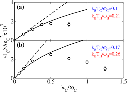
Figure 3: Dependence of the steady-state heat current $I_{C}$ on TLS-bath coupling strength $\lambda_{C}$. Panels (a) and (b) correspond to different temperatures of baths. The spectral densities for the two baths are equal ($\lambda_{C}=\lambda_{H}$, $\omega_{C}=\omega_{H}$). The TLS energy spacing is $\epsilon/\omega_{C}=0.75$. The numerical results have been obtained with the numerically exact ML-MCTDH methodology (circles), the Segal-Nitzan theory (dashed lines), and the NEGF-Redfield approach developed in this work (full lines). Error bars for some numerically exact points are smaller than the size of circles, and, therefore, not shown in the figure.

The bath parameters in Eq. (37), i.e., the TLS-bath coupling strength and the characteristic frequency, are chosen to be identical for the two baths, i.e., $\lambda_{C}=\lambda_{H}$ and $\omega_{C}=\omega_{H}$, respectively. The bath temperatures are defined by $k_{B}T_{C}/\omega_{C}=0.1$, $k_{B}T_{H}/\omega_{H}=0.21$ for the cold and the hot bath in panel (a) and $k_{B}T_{C}/\omega_{C}=0.17$, $k_{B}T_{H}/\omega_{H}=0.26$ for the cold and the hot bath in panel (b), respectively. The ratio of the TLS energy spacing to the characteristic frequency of the bath is taken as $\epsilon/\omega_{C}=0.75$ in both panels.

The numerical results of the NEGF-Redfield and Segal-Nitzan methods are obtained from Eq. (42) and Eq. (43), respectively. The numerically exact results are obtained by means of the Multilayer Multiconfiguration Time-Dependent Hartree (ML-MCTDH) approach.Wang2003-1289 The details on the application of the ML-MCTDH method to the study of heat transport in the SBNM are described elsewhere.Velizhanin2008-325 For the parameters considered here both the NEGF-Redfield and Segal-Nitzan theories, depicted by the dashed and full black lines, perform well if $\lambda_{C}$ is sufficiently small. However, when $\lambda_{C}/\omega_{C}$ is larger than $\sim 0.5$, both approximate theories cease to be valid and the results deviate significantly from the numerically exact simulation. This failure is expected considering the weak-coupling nature of the approximations in both approximate methods. In the intermediate region ($\lambda_{C}/\omega_{C}\approx$ 0.3-0.5) the NEGF-Redfield method gives significantly better results than the Segal-Nitzan approach, because the former treats the TLS-bath coupling more accurately as was discussed in the previous section.

At large coupling strengths the numerically exact simulation predicts a “turnover”,Hanggi1990-251 ; Pollak2000-1 ; Velizhanin2008-325 i.e., the heat current reaches its maximum and starts to decrease with increasing of the coupling strength. This phenomenon is similar to Kramers’ turnover and has been discussed in more detail elsewhere.Velizhanin2008-325 The turnover is not reproduced (even qualitatively) by the approximate theories although the NEGF-Redfield method displays the correct curvature change in the intermediate coupling regime.

The accuracy of the NEGF-Redfield approach deteriorates significantly if the self-consistency constraint, Eq. (44), is not applied and the steady-state populations are obtained from regular Redfield theory, i.e., from Eq. (30). The heat currents from the bridge to the cold bath, $\langle I_{C}\rangle$, and from the hot bath to the bridge, $-\langle I_{H}\rangle$, evaluated for this choice of the steady-state populations, are depicted by up-triangles and down-triangles, respectively, in Fig. 4(a).

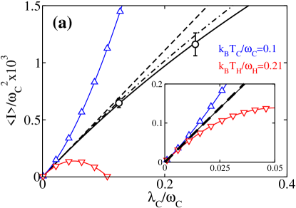
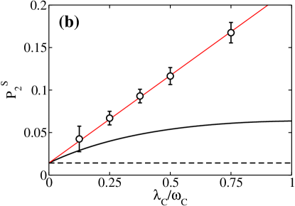
Figure 4: Dependence of the steady-state heat current (Panel a) and the steady-state population of the higher TLS level (Panel b) on the TLS-bath coupling strength $\lambda_{C}$. All parameters are the same and circles, full lines and dashed lines correspond to the same theoretical methods as in Fig. 3(a). The up-triangles and down-triangles depict $\langle I_{C}\rangle$ and $-\langle I_{H}\rangle$, respectively, in the case when steady-state populations are obtained directly from the Redfield master equation, Eq. (30), and not from the self-consistency requirement, Eq. (44). The average of these two currents, i.e., $(\langle I_{C}\rangle-\langle I_{H}\rangle)/2$, is depicted by the dashed-dotted line. The thin red line in Panel b, which was obtained by fitting the numerically exact results, is a guide for the eye.

In the inset, it is seen that at very small coupling strength these two currents coincide with each other and with the current determined self-consistently. However, $\langle I_{C}\rangle$ and $-\langle I_{H}\rangle$ start to deviate from each other at $\lambda_{C}/\omega_{C}\approx 0.01$, thus demonstrating the non-conservation of the energy current discussed above. Furthermore, the heat current from the hot bath to the bridge becomes unphysically negative at $\lambda_{C}/\omega_{C}\approx 0.1$.

The energy conservation condition in Eq. (44) suggests another, more symmetric, definition of heat current by averaging $\langle I_{C}\rangle$ and $-\langle I_{H}\rangle$, i.e., $(\langle I_{C}\rangle-\langle I_{H}\rangle)/2$.Velizhanin2008-325 This averaged current, with $\langle I_{C}\rangle$ and $-\langle I_{H}\rangle$ given by up- and down-triangles, respectively, is depicted by the dashed-dotted line in Fig. 4. This current is seen to agree much better with the numerically exact results than $\langle I_{C}\rangle$ and $-\langle I_{H}\rangle$ separately. However, this “averaging” trick does not resolve the energy non-conservation problem, and merely conceals it. Furthermore, the NEGF-Redfield approach with self-consistency introduced (full line) is still in better agreement with the numerically exact calculations. Therefore, the results of Fig. 4(a) emphasize the necessity of the energy conservation requirement and support our choice of the steady-state populations.

This choice is further supported by Fig. 4(b), where the steady-state population of the higher TLS state, evaluated from Eq. (44) within the NEGF-Redfield theory (full line), Redfield master equation (dashed line) and the numerically exact simulation (circles), is depicted. Whereas standard Redfield theory (dashed line) yields a population $P^{S}_{2}$ that is totally independent on the coupling strength, the NEGF-Redfield theory performs better reproducing, although not quantitatively, the increase of the population with $\lambda_{C}$.

The influence of the TLS energy spacing $\epsilon$ on the steady-state heat current in shown in Figure 5.

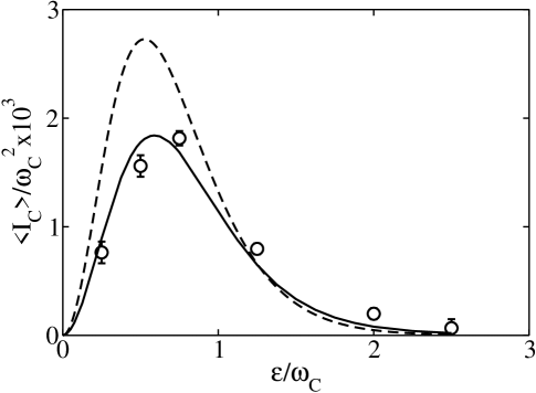
Figure 5: Dependence of steady-state heat current $I_{C}$ on the TLS energy spacing $\epsilon$. The results have been obtained with the numerically exact ML-MCTDH method (circles), the Segal-Nitzan theory (dashed line), and the NEGF-Redfield approach (full line). The temperatures are $k_{B}T_{C}/\omega_{C}=0.17$ and $k_{B}T_{H}/\omega_{H}=0.26$ ($\omega_{C}=\omega_{H}$). The TLS-bath coupling strength is $\lambda_{C}/\omega_{C}=0.25$ ($\lambda_{C}=\lambda_{H}$). Error bars for some numerically exact points are smaller than the size of circles, and, therefore, not shown in the figure.

As is seen, the heat current also exhibits a turnover behavior as a function of the energy spacing. This is due to the resonant character of heat transport: The heat transport is most efficient if the TLS has the same characteristic frequency, i.e., energy spacing between the two levels, as that of the baths. Too large or too small $\epsilon$ (compared to $\omega_{c}$) both result in inefficient heat transfer. The detailed discussion of this phenomenon is given elsewhere.Velizhanin2008-325

While the Segal-Nitzan theory can qualitatively predict this turnover behavior, there is a significant quantitative discrepancy with the numerically exact simulation. However, the NEGF-Redfield theory method is in much better agreement with the numerically exact results in Fig. 5. We attribute this to the fact that since the coupling strength is relatively small ($\lambda_{C}/\omega_{C}=0.25$), a more accurate treatment of TLS-bath coupling within the NEGF-Redfield approach leads to a much better agreement with the numerically exact result.

IV Concluding Remarks

In this paper we have derived an analog of the Meir-Wingreen formula for a spin-boson nanojunction model for heat transport in a single-molecule junction. This formula exactly relates the steady-state heat current through a two-level system, connected to two heat reservoirs, to correlation functions of the operators of the two-level system only. The formula allows one to calculate the steady-state heat current for the spin-boson nanojunction model using previously developed methodologies for the reduced dynamics of the standard spin-boson problem.

As an illustrative application of the formalism developed, we have analyzed the properties of the steady-state heat conduction in the spin-boson nanojunction model using the derived expression for the heat current and Redfield theory to evaluate the correlation functions of the two-level system. In addition, a self-consistency criterion was formulated and applied that enforces the conservation of the heat current within the NEGF-Redfield scheme. Employing this approach, we have studied the dependence of the heat current on the energy spacing of the two level-system and the coupling strength between the system and the heat baths. The numerical results obtained in this work demonstrated that the NEGF-Redfield method represents a significant improvement compared to previous approaches due to the more accurate treatment of the coupling between the two-level system and the heat baths.

Finally, we would like to comment on the relation of the Meir-Wingreen formula (24) developed in this work to previously developed NEGF-based theories of thermal transport. The latter theories are based on the phonon picture and the anharmonicity, i.e., phonon-phonon interactions, is included perturbatively (see Ref. Wang2008-381, for an excellent review and references therein). In contrast, Eq. (24) treats in-bridge anharmonicity non-perturbatively since exact eigenstates of an anharmonic oscillator can serve as bridge levels. For example, the two levels considered in this may model the two lowest eigenstates of a double-well potential, which often cannot be treated perturbatively. On the other hand, an eigenstate expansion is limited to a relatively small bridge including only few vibrational modes. Thus, the approach developed in this paper has to be extended and optimized to apply it to large molecular bridges. Therefore, the method developed in this work and the conventional NEGF-based theories of heat transport are independent and complementary. A major improvement in the theory of heat transport through nanojunctions can thus be expected if the two methods are combined, allowing the simultaneous treatment of weakly and highly anharmonic modes of the same nanojunction by anharmonic perturbation theory and exact diagonalization methods, respectively.

- (1) M. J. Montgomery, T. N. Todorov, and A. P. Sutton, J. Phys. Condens. Matter 14, 5377 (2002).
- (2) Y. C. Chen, M. Zwolak, and M. D. Ventra, Nano Lett. 3, 1691 (2003).
- (3) D. Segal, A. Nitzan, and P. Hanggi, J. Chem. Phys. 119, 6840 (2003).
- (4) Z. F. Huang, B. Q. Xu, Y. C. Chen, M. D. Ventra, and N. J. Tao, Nano Lett. 6, 1240 (2006).
- (5) A. Pecchia, G. Romano, and A. D. Carlo, Phys. Rev. B 75, 035401 (2007).
- (6) Z. Ioffe, T. Shamai, A. Ophir, G. Noy, I. Yutsis, K. Kfir, O. Chesnovsky, and Y. Selzer, Nature Nano. 3, 727 (2008).
- (7) R. Härtle, C. Benesch, and M. Thoss, Phys. Rev. Lett. 102, 146801 (2009).
- (8) D. Segal and A. Nitzan, Phys. Rev. Lett. 94, 034301 (2005).
- (9) D. Segal and A. Nitzan, J. Chem. Phys. 122, 194704 (2005).
- (10) D. Segal and A. Nitzan, Phys. Rev. E 73, 026109 (2006).
- (11) A. G. Redfield, IBM J. Res. Dev. 1, 19 (1957).
- (12) A. G. Redfield, Adv. Magn. Reson. 1, 1 (1965).
- (13) K. A. Velizhanin, H. Wang, and M. Thoss, Chem. Phys. Lett. 460, 325 (2008).
- (14) H. Wang and M. Thoss, J. Chem. Phys. 119, 1289 (2003).
- (15) A. J. Leggett, S. Chakravarty, A. T. Dorsey, M. P. A. Fisher, A. Garg, and W. Zwerger, Rev. Mod. Phys. 59, 1 (1987).
- (16) U. Weiss, Quantum Dissipative Systems (World Scientific, Singapore, 1999).
- (17) C. Aslangul, N. Pottier, and D. Saint-James, J. Phys (Paris) 47, 1657 (1986).
- (18) L. Zusman, Chem. Phys. 49, 295 (1980).
- (19) J. Ankerhold and H. Lehle, J. Chem. Phys. 120, 1436 (2004).
- (20) Y. Meir and N. S. Wingreen, Phys. Rev. Lett. 68, 2512 (1992).
- (21) J. Schwinger, J. Math. Phys. 2, 407 (1961).
- (22) L. V. Keldysh, Sov. Phys. JETP 20, 1018 (1965).
- (23) M. Gaudin, Nucl. Phys 15, 89 (1960).
- (24) A. Fetter and J. Walecka, Quantum Theory of Many-Particle Physics (McGraw-Hill, New York, 1971), 1st ed.
- (25) A. P. Jauho, N. S. Wingreen, and Y. Meir, Phys. Rev. B 50, 5528 (1994).
- (26) H. Haug and A. P. Jauho, Quantum Kinetics in Transport and Optics of Semiconductors (Springer-Verlag, Berlin, 1996).
- (27) H. Bruus and K. Flensberg, Many-Body Quantum Theory in Condensed Matter Physics (Oxford University Press, New York, 2004), 1st ed.
- (28) M. Esposito and M. Galperin, Phys. Rev. B 79, 205303 (2009).
- (29) G. D. Mahan, Many-Particle Physics (Kluwer Academic/Plenum Publishers, New York, 2000), 3rd ed.
- (30) T. Ojanen and A.-P. Jauho, Phys. Rev. Lett. 100, 155902 (2008).
- (31) T. Ruokola, T. Ojanen, and A.-P. Jauho, Phys. Rev. B 79, 144306 (2009).
- (32) G. Baym and L. P. Kadanoff, Phys. Rev. 124, 287 (1961).
- (33) G. Baym, Phys. Rev. 127, 1391 (1962).
- (34) P. Hänggi, P. Talkner, and M. Borkovec, Rev. Mod. Phys. 62, 251 (1990).
- (35) E. Pollak, in Theoretical Methods in Condensed Phase Chemistry, edited by S. D. Scwhartz (Kluwer, The Netherlands, 2000), p. 1.
- (36) J.-S. Wang, J. Wang, and J. T. Lü, Eur. Phys. J. B 62, 381 (2008).