Continuous symmetry reduction and return maps for high-dimensional flows

Abstract

We present two continuous symmetry reduction methods for reducing high-dimensional dissipative flows to local return maps. In the Hilbert polynomial basis approach, the equivariant dynamics is rewritten in terms of invariant coordinates. In the method of moving frames (or method of slices) the state space is sliced locally in such a way that each group orbit of symmetry-equivalent points is represented by a single point. In either approach, numerical computations can be performed in the original state-space representation, and the solutions are then projected onto the symmetry-reduced state space. The two methods are illustrated by reduction of the complex Lorenz system, a 5-dimensional dissipative flow with rotational symmetry. While the Hilbert polynomial basis approach appears unfeasible for high-dimensional flows, symmetry reduction by the method of moving frames offers hope.

1 Introduction

In his seminal paper, E. Lorenz [1] reduced the continuous time and discrete spatial symmetries of the 3-dimensional Lorenz equations, resulting in a 1-dimensional return map that yields deep insights [2] into the nature of chaos in this flow. For strongly contracting, low-dimensional flows, Gilmore, Lefranc and Letellier [3, 4] systematized construction of such discrete time return maps, through use of topological templates, Poincaré sections (to reduce the continuous time invariance) and invariant polynomial bases (to reduce the spatial symmetries). They showed that in presence of spatial symmetries one has to ‘quotient’ the symmetry and replace the dynamics by a physically equivalent reduced, desymmetrized flow, in which each family of symmetry-related states is replaced by a single representative. This approach leads to symbolic dynamics and labeling of all periodic orbits up to a given topological period. Periodic orbit theory can then yield accurate estimates of long-time dynamical averages, such as Lyapunov exponents and escape rates [5].

In a series of papers Cvitanović, Putkaradze, Christiansen and Lan [6, 7, 8, 9, 10, 11] showed that effectively low-dimensional return maps can be constructed for high-dimensional (formally infinite dimensional) flows described by dissipative partial differential equations (PDEs) such as the Kuramoto-Sivashinsky equation (KS). Such flows have state-space topology vastly more complicated than the Lorenz flow, and collections of local Poincaré sections together with maps from a section to a section are required to capture all of the important asymptotic dynamics. These KS studies were facilitated by a restriction to the flow-invariant subspace of odd solutions, but at a price: elimination of the translational symmetry of the KS system and with it physically important phenomena, such as traveling waves. Traveling (or relative) unstable coherent solutions are ubiquitous and play a key role in organization of turbulent hydrodynamic flows, as pointed already in 1982 by Rand [12], and confirmed both by simulations and experimentation [13, 14, 15, 16, 17, 18]. For KS [19, 20], and even for a relatively low-dimensional flow such as the complex Lorenz equations [21, 22] used as an example here, with the simplest possible continuous (rotational) spatial symmetry, the symmetry-induced drifts obscure the underlying hyperbolic dynamics.

The question that we address here is how one can construct suitable return maps for arbitrarily high-dimensional but strongly dissipative flows in presence of continuous symmetries. Our exposition is based in part on refs. [20, 5, 23]. The reader is referred to Golubitsky and Stewart [24], Hoyle [25], Olver [26], Bredon [27], and Krupa [28] for more depth and rigor than would be wise to wade into here.

In sect. 2 we review the basic notions of symmetry in dynamics. Sect. 2.1 introduces the $\textrm{SO}(2)$ equivariant complex Lorenz equations (CLE), a 5-dimensional set of ODEs that we use throughout the paper to illustrate the strengths and drawbacks of different symmetry reduction methods. In sect. 3 we describe important classes of solutions and their symmetries: equilibria, relative equilibria, periodic and relative periodic orbits, and use them to motivate the need for symmetry reduction.

In sect. 4 we describe the problem of symmetry reduction. The action of a symmetry group endows the state space with the structure of a union of group orbits, each group orbit an equivalence class. The goal of symmetry reduction is replace each group orbit by a unique point a lower-dimensional reduced state space. In sect. 5 we briefly review the standard approach to spatial symmetry reduction, projection to a Hilbert basis, and explain why we find it impracticable. In sect. 6 we review the method of moving frames, a direct and efficient method for computing symmetry-invariant bases that goes back to Cartan, and in sect. 6.1 we apply the method to the complex Lorenz equations. The method maps all solutions to a slice, a submanifold of state space that plays a role for group orbits akin to the role Poincaré sections play in reducing continuous time invariance. In contrast to the Hilbert basis approach, slices are local, with a generic trajectory within a slice bound to encounter singularities, and more than one slice might be needed to capture the flow globally. In sect. 6.2 we show that a single local slice can suffice for the purpose of reducing the complex Lorenz equations flow to a return map. In sect. 7 we recast the method of moving frames into the equivalent, differential method of slices, with time integration restricted to a slice fixed by a given state space point.

2 Symmetries of dynamical systems

Here we are interested in the role continuous symmetries play in dynamics. The methods we develop are in principle applicable to to translational and rotational symmetries of ODEs and PDEs, described by compact or noncompact Lie groups. We have in mind applications to PDEs such as Kuramoto-Sivashinsky and plane Couette flow which exhibit translational symmetries in either infinite or periodic domains. In the former case the group of symmetries is Euclidean and noncompact, and in the latter case orthogonal and compact. In numerical computations the periodic setting is usually considered and, though Fourier analysis, a translation is represented by the action of the 1-parameter Lie $\textrm{SO}(2)$ group on its linearly irreducible subspaces, the Fourier modes. Through truncation (for example spectral discretization), PDEs are transformed to high- but finite-dimensional systems of ODEs. The key concepts will thus be illustrated by a specific ODE example, the $\textrm{SO}(2)$ group acting on a five-dimensional state space, linearly decomposable into a direct sum of irreducible subspaces of $\textrm{SO}(2)$.

Consider a system of ODEs of the form

$$\dot{x}=v(x)$$ (1)

with $v$ a smooth vector field and $x\in{\cal M}\subset\mathbb{R}^{d}$.

A linear action $g$ is a symmetry of (1) if

$$v(gx)=g\,v(x)$$ (2)

for all $x\in\mathbb{R}^{d}$. One says that $v$ commutes with $g$ or that $v$ is $g$-equivariant. When $v$ commutes with the set of group elements $g\in G$, the vector field $v$ is said to be $G$-equivariant. The group $G$ is said to be a symmetry of dynamics if for every solution $x(\tau)={f^{\tau}(x)}$, $g\,x(\tau)$ is also a solution. The finite time flow ${f^{\tau}(gx)}$ through $gx$ then satisfies the equivariance condition

$${f^{\tau}(gx)}=g{f^{\tau}(x)}\,.$$ (3)

In physics literature the term $in\-vari\-ant$ is most commonly used; for example, in Hamiltonian systems a symmetry is manifested as invariance of the Hamiltonian under the symmetry group action.

An element of a compact Lie group continuously connected to identity can be written as

$$g({\bf\theta})=e^{{\bf\theta}\cdot\mathbf{T}}\,,\qquad{\bf\theta}\cdot\mathbf{T}=\sum{\bf\theta}_{a}\mathbf{T}_{a},\;a=1,2,\cdots,N\,,$$ (4)

where ${\bf\theta}\cdot\mathbf{T}$ is a Lie algebra element, and ${\bf\theta}_{a}$ are the parameters of the transformation. Repeated indices are summed throughout this chapter, and the dot product refers to a sum over Lie algebra generators. The Euclidian product of two vectors $x,y$ is indicated by $x$-transpose times $y$, i.e., $x^{T}y=\sum_{i}^{d}x_{i}y_{i}$. Finite transformations $\exp({\bf\theta}\cdot{\mathbf{T}})$ are generated by sequences of infinitesimal steps of form

$$g(\delta{\bf\theta})\simeq 1+\delta{\bf\theta}\cdot\mathbf{T}\,,\quad\delta{\bf\theta}\in\mathbb{R}^{N}\,,\quad|\delta{\bf\theta}|\ll 1\,,$$ (5)

where $\mathbf{T}_{a}$, the generators of infinitesimal transformations, are a set of $N$ linearly independent $[d\!\times\!d]$ anti-hermitian matrices, $(\mathbf{T}_{a})^{\dagger}=-\mathbf{T}_{a}$, acting linearly on the $d$-dimensional state space ${\cal M}$. For $G\subset\textrm{O}(n)$ the generators can always be brought to real, antisymmetric form $\mathbf{T}^{T}=-\mathbf{T}$. The flow induced by the action of the group on the state space point $x$ is given by the set of $N$ tangent fields

$$t_{a}(x)_{i}=(\mathbf{T}_{a}){}_{ij}x_{j}\,.$$ (6)

These tangent fields are always normal to the ‘radial’ vector $x$,

$$x^{T}t_{a}(x)=0\,.$$ (7)

For an infinitesimal transformation (5) the $G$-equivariance condition (2) becomes

$$v(x)\simeq(1-{\bf\theta}\cdot\mathbf{T})\,v(x+{\bf\theta}\cdot\mathbf{T}\,x)=v(x)-{\bf\theta}\cdot\mathbf{T}\,v(x)+\frac{dv}{dx}\,{\bf\theta}\cdot\mathbf{T}\,x\,.$$

Thus the infinitesimal, Lie algebra $G$-equivariance condition is

$$t_{a}(v)-A(x)\,t_{a}(x)=0\,,$$ (8)

where $A={\partial v}/{\partial x}$ is the stability matrix. The left-hand side,

$${\cal L}_{t_{a}}v=\left.\left(\mathbf{T}_{a}-\frac{\partial}{\partial y}(\mathbf{T}_{a}x)\right)v(y)\right|_{y=x}\,,$$ (9)

is known as the Lie derivative of the dynamical flow field $v$ along the direction of the infinitesimal group-rotation induced flow $t_{a}(x)=\mathbf{T}_{a}x$. The equivariance condition (8) states that the two flows, one induced by the dynamical vector field $v$, and the other by the group tangent field $t$, commute if their Lie derivatives (or the Lie brackets or Poisson brackets) vanish.

Any representation of a compact Lie group $G$ is fully reducible, and invariant tensors constructed by contractions of $\mathbf{T}_{a}$ are useful for identifying irreducible representations. The simplest such invariant is bilinear,

$$\mathbf{T}^{T}\cdot\mathbf{T}=\sum_{\alpha}C_{2}^{(\alpha)}\,{\ \hbox{{\rm 1}\kern-6.00006pt\hbox{\rm 1}}}^{(\alpha)}\,,$$ (10)

where $C_{2}^{(\alpha)}$ is the quadratic Casimir for irreducible representation labeled $\alpha$, and ${\ \hbox{{\rm 1}\kern-6.00006pt\hbox{\rm 1}}}^{(\alpha)}$ is the identity on the $\alpha$-irreducible subspace, 0 elsewhere. The dot product of two tangent fields is thus a sum weighted by Casimirs,

$$t(x)^{T}\cdot t(x^{\prime})=\sum_{\alpha}C_{2}^{(\alpha)}x_{i}\,\delta_{ij}^{(\alpha)}x^{\prime}_{j}\,.$$ (11)

If $x$ is not invariant (fixed under group actions), $t(x)^{T}\cdot t(x)$ is strictly positive. $t(x)^{T}\cdot t(x^{\prime})$, however, can take either sign, or even vanish.

2.1 An example: Complex Lorenz equations

Consider a complex generalization of Lorenz equations,

$$\dot{x} = -\sigma x+\sigma y\,,\qquad\dot{y}\,=\,(\rho-z)x-ay$$

$$\dot{z} = (xy^{*}+x^{*}y)/2-bz\,,$$ (12)

where $x,y$ are complex variables, $z$ is real, while the parameters $\sigma,\,b$ are real and $\rho=\rho_{1}+i\rho_{2}$, $a=1-ie$ are complex. Recast in real variables, $x=x_{1}+ix_{2}\,,\,y=y_{1}+iy_{2}$ this is a set of five coupled ODEs

$$\dot{x}_{1} = -\sigma x_{1}+\sigma y_{1}\,,\quad\dot{x}_{2}\,=\,-\sigma x_{2}+\sigma y_{2}$$

$$\dot{y}_{1} = (\rho_{1}-z)x_{1}-\rho_{2}x_{2}-y_{1}-ey_{2}$$

$$\dot{y}_{2} = \rho_{2}x_{1}+(\rho_{1}-z)x_{2}+ey_{1}-y_{2}$$

$$\dot{z}\; = -bz+x_{1}y_{1}+x_{2}y_{2}\,.$$ (13)

In all numerical examples that follow, the parameters will be set to $\rho_{1}=28,\,\rho_{2}=0,\,b=8/3,\,\sigma=10,\,e=1/10$, unless explicitly stated otherwise.

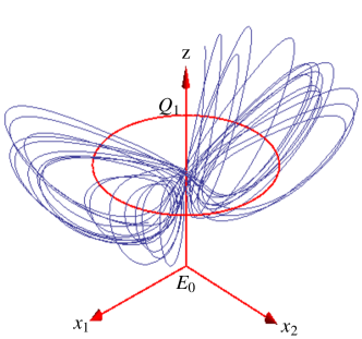
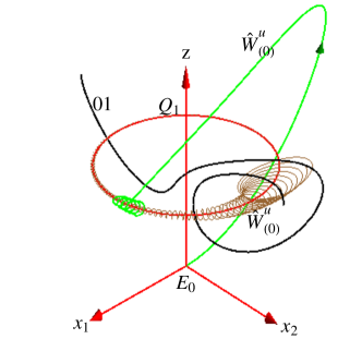
Figure 1: State space portrait of complex Lorenz flow. Plotted are a generic chaotic trajectory (blue), the $\mathrm{E}_{0}$ equilibrium, a representative of its unstable manifold (green), the $\mathrm{Q}_{1}$ relative equilibrium (red), its unstable manifold (brown), and one repeat of the $\overline{01}$ relative periodic orbit (black) (color online).

Why worry about continuous symmetries? The visualization in figure 1 of typical long-time dynamics of complex Lorenz flow suffices to illustrate the effect a continuous symmetry has on dynamics. A generic trajectory slowly drifts along the direction of continuous symmetry while tracing a Lorenz-butterfly like attractor. It is a mess.

The complex Lorenz equations are a dynamical system with a continuous (but no discrete) symmetry, equivariant under the one-parameter rotation group $\textrm{U}(1)\cong\textrm{SO}(2)$ acting by

$$(x,\,y,\,z)\mapsto(e^{i\theta}x,\,e^{i\theta}y,\,z)\,,\ \theta\in[0,2\pi]\,.$$ (14)

Alternatively, substituting the Lie algebra generator

$$\mathbf{T}\,=\,\left(\begin{array}[]{ccccc}0&-1&0&0&0\\ 1&0&0&0&0\\ 0&0&0&-1&0\\ 0&0&1&0&0\\ 0&0&0&0&0\end{array}\right)$$ (15)

acting on a 5-dimensional space (13) into (4) yields the $\mathbb{R}^{5}$ representation of a finite angle action (14) of $\textrm{SO}(2)$

$$g({\bf\theta})\,=\,\left(\begin{array}[]{ccccc}\cos{\bf\theta}&-\sin{\bf\theta}&0&0&0\\ \sin{\bf\theta}&\cos{\bf\theta}&0&0&0\\ 0&0&\cos{\bf\theta}&-\sin{\bf\theta}&0\\ 0&0&\sin{\bf\theta}&\cos{\bf\theta}&0\\ 0&0&0&0&1\end{array}\right)\,.$$ (16)

We see that the linear action of $\textrm{SO}(2)$ on the state space of the complex Lorenz equations decomposes into the $m\!=\!0$ $G$-invariant subspace ($z$-axis) and the $m=1$ subspace of multiplicity 2.

The generator $\mathbf{T}$ is anti-symmetric, $\mathbf{T}^{T}=-\mathbf{T}$, and the group is compact, its elements parametrized by ${\bf\theta}\mbox{ mod }2\pi$. Locally, at $x\in{\cal M}$, the infinitesimal action of the group is given by the group tangent field $t(x)=\mathbf{T}x=(-x_{2},x_{1},-y_{2},y_{1},0)$. In other words, the flow induced by the group action is normal to the radial direction in the $(x_{1},x_{2})$ and $(y_{1},y_{2})$ planes, while the $z$-axis is left invariant.

The equivariance of the complex Lorenz flow under $\textrm{SO}(2)$ rotations (16) can be verified by substituting the Lie algebra generator (15) and the stability matrix for complex Lorenz flow (13),

$$A=\left(\begin{array}[]{ccccc}-\sigma&0&\sigma&0&0\\ 0&-\sigma&0&\sigma&0\\ \rho_{1}-z&-\rho_{2}&-1&-e&-x_{1}\\ \rho_{2}&\rho_{1}-z&e&-1&-x_{2}\\ y_{1}&y_{2}&x_{1}&x_{2}&-b\end{array}\right)\,,$$ (17)

into the equivariance condition (8). For the parameter values (13) the flow is strongly volume contracting,

$$\partial_{i}v_{i}=\mbox{\rm tr}\,A=\sum_{i=1}^{5}\lambda_{i}(x,t)=-b-2(\sigma+1)=-24-2/3\,.$$ (18)

The complex Lorenz equations (12) were introduced by Gibbon and McGuinness [21, 22] as a low-dimensional model of baroclinic instability in the atmosphere. Zeghlache and Mandel [29] and Ning and Haken [30] have shown that equations isomorphic to the complex Lorenz equations, with $e+\rho_{2}=0$, also appear as a truncation of Maxwell-Bloch equations describing a single mode, detuned, ring laser. The choice $e+\rho_{2}=0$ is degenerate (see (22)) in the sense that it leads to non-generic bifurcations. We follow Bakasov and Abraham [31] who set $\rho_{2}=0$ and $e\neq 0$ to describe detuned ring lasers.

Here, however, we are not interested in the physical applications of these equations; rather, we study them as a simple example of a dynamical system with continuous (but no discrete) symmetries, with a view of testing methods of reducing the dynamics to a lower-dimensional reduced state space. We investigate various ways of quotienting its $\textrm{SO}(2)$ symmetry, and reducing the dynamics to a 4-dimensional reduced state space. As we shall show, the dynamics has a nice ‘stretch & fold’ action, but that is totally masked by the continuous symmetry drifts. We shall not rest until we attain the simplicity of figure 6, and the bliss of 1-dimensional return map of figure 4.

3 Symmetries of solutions

In order to explore the implications of equivariance on solutions of dynamical equations, we start by examining the way a compact Lie group acts on a state space ${\cal M}$. The group orbit or $G$-orbit of the point $x\in{\cal M}$ is the set

$${\cal M}_{x}=\{g\,x\mid g\in{G}\}$$ (19)

of all state space points into which $x$ is mapped under the action of $G$. The symmetry $G_{x}$ (isotropy or stabilizer group) of a state space point $x$ is the largest subgroup of $G$

$$G_{x}=\{g\in G:gx=x\}$$ (20)

that leaves $x$ fixed. The symmetry $G_{X}$ of a set ${\cal M}_{X}\in{\cal M}$ is the largest subgroup of $G$ that leaves ${\cal M}_{X}$ invariant as a set:

$$G_{X}=\{g:g\,{\cal M}_{X}={\cal M}_{X}\}\,.$$

If $G_{p}$ is a symmetry, intrinsic properties of a solution ${\cal M}_{p}$ (such as equilibrium or a cycle stability eigenvalues, period, Floquet multipliers) evaluated anywhere along its $G_{p}$-orbit are the same. A symmetry thus reduces the number of inequivalent solutions. So we also need to describe the symmetry of a solution, as opposed to (3), the symmetry of the system.

The fixed-point subspace $\mathrm{Fix}\left(H\right)$ of a subgroup $H\subset G$ is the subspace of ${\cal M}$ containing all fixed points of $H$:

$$\mathrm{Fix}\left(H\right)=\{x\in{\cal M},\,g\in H\,|\,gx=x\}\,.$$

The physical importance of fixed-point subspaces lies in the fact that they are invariant under $G$-equivariant dynamics [24],

$$f^{\tau}\left(\mathrm{Fix}\left(H\right)\right)\subseteq\mathrm{Fix}\left(H\right)$$

and thus flow invariant for all times $\tau$. Therefore if $x(\tau)$ is a solution of an equivariant ODE, then its symmetry $G_{x(\tau)}=G_{x(0)}$ is preserved for all times.

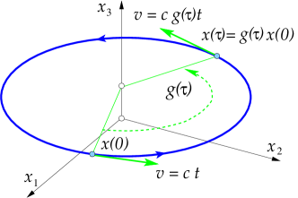
(a)  (b)

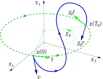
Figure 2: (a) A relative equilibrium orbit starts at some point $x(0)$, with the dynamical flow field $v(x)=c\cdot t(x)$ pointing along the group tangent space. For the $\textrm{SO}(2)$ symmetry depicted here, the flow traces out the group orbit of $x(0)$ in time ${T}=2\pi/c$. An equilibrium lives either in the $\mathrm{Fix}\left(G\right)$ subspace ($x_{3}$ axis in this sketch), or on a group orbit as the one depicted here, but with zero angular velocity $c$. In the latter case the circle (in general, $N$-torus) depicts a continuous family of fixed equilibria, related only by the group action. (b) A relative periodic orbit starts out at $x(0)$ with the dynamical $v$ and group tangent $t$ flows pointing in different directions, and returns to the group orbit of $x(0)$ after time ${T_{p}}$ at $x({T_{p}})=g_{p}x(0)$, a rotation of the initial point by $g_{p}$.

In contrast to equilibrium solutions that satisfy $f^{\tau}(x)=x$, relative equilibria (or traveling waves) satisfy $f^{\tau}(x)=g(\tau)\,x$ for any $\tau$, where the group has been reparameterized by time, $\theta=\theta(\tau)$. In a co-moving frame moving along the group orbit with velocity $v(x)=c\cdot t(x)$, the relative equilibrium appears as an equilibrium. Here $t$ is the group tangent field (6).

A relative periodic orbit is an orbit ${\cal M}_{p}$ for which the initial point exactly recurs

$$x_{p}(0)=g_{p}x_{p}({T_{p}})\,,\qquad x_{p}(\tau)\in{\cal M}_{p}\,,$$ (21)

at a fixed relative period ${T_{p}}$, but shifted by a fixed group action ${g_{p}}$ which brings the endpoint $x_{p}({T_{p}})$ back into the initial point $x_{p}(0)$, see figure 2 (b). The group action ${g_{p}}=g_{p}({\bf\theta})$ parameters ${\bf\theta}_{p}=({\bf\theta}_{1},{\bf\theta}_{2},\cdots{\bf\theta}_{N})$ will be referred to as phases, or shifts. For dynamical systems with only continuous (no discrete) symmetries, the parameters $\{t,{\bf\theta}_{1},\cdots,{\bf\theta}_{N}\}$ are real numbers, the ratios $\pi/{\bf\theta}_{j}$ are almost never rational, and the likelihood of closing into a periodic orbit is zero. Thus the trajectory of a relative periodic orbit generically sweeps out the group orbit ergodically.

(a)  (b)

Figure 3: A relative periodic orbit of the Kuramoto-Sivashinsky flow, traced for four periods ${T_{p}}$ and projected on (a) a stationary state space coordinate frame $\{v_{1},v_{2},v_{3}\}$; (b) a co-moving $\{\tilde{v}_{1},\tilde{v}_{2},\tilde{v}_{3}\}$ coordinate frame, moving with the mean velocity $c_{p}={\bf\theta}_{p}/{T_{p}}$. (From ref. [19].)

A relative periodic orbit is periodic in its mean velocity $c_{p}={\bf\theta}_{p}/{T_{p}}$ co-rotating frame, figure 3, but in the stationary frame its trajectory is quasiperiodic. A co-moving frame is helpful in visualizing a single ‘relative’ orbit, but useless for viewing collections of orbits, as each one drifts with its own group velocity. A simultaneous visualization of all relative periodic orbits as periodic orbits can be attained only by symmetry reduction, to be undertaken in sects. 5 and 6.

Relative equilibria and relative periodic orbits are the hallmark of systems with continuous symmetry. Amusingly, in this extension of periodic orbit theory from unstable 1-dimensional closed periodic orbits to unstable $(N\!+\!1)$-dimensional compact manifolds ${\cal M}_{p}$ invariant under continuous symmetries, there are either no or proportionally few periodic orbits. In presence of a continuous and no discrete symmetry, likelihood of finding a periodic orbit is zero. Relative periodic orbits are almost never eventually periodic, i.e., they almost never lie on periodic trajectories in the full state space, so looking for periodic orbits in systems with only continuous symmetries is a fool’s errand.

A historical note. Relative equilibria and relative periodic orbits are related to equilibria and periodic orbits of dynamics reduced by the symmetries. They appear in many physical situations, such as motion of rigid bodies, gravitational $N$-body problems, molecules, nonlinear waves, spiralling patterns and turbulence. According to Cushman, Bates [32] and Yoder [33], C. Huygens [34] understood the relative equilibria of a spherical pendulum many years before publishing them in 1673. A reduction of the translation symmetry was obtained by Jacobi (for a modern, symplectic implementation, see Laskar et al. [35]). According to Chenciner [36], the first attempt to find (relative) periodic solutions of the $N$-body problem was the 1896 short note by Poincaré [37], in the context of the 3-body problem. Relative equilibria of the $N$-body problem (known in this context as Lagrange points, stationary in the co-rotating frame) are circular motions in the inertial frame, and relative periodic orbits correspond to quasiperiodic motions in the inertial frame. Relative equilibria that exist in a rotating frame are called central configurations. For relative periodic orbits in celestial mechanics see also ref. [38]. A striking application of relative periodic orbits has been the discovery of ‘choreographies’ of $N$-body problems [39, 40, 41].

The modern story on equivariance and dynamical systems starts perhaps with M. Field [42], and on bifurcations in presence of symmetries with Ruelle [43]. Ruelle proves that the stability matrix/Jacobian matrix evaluated at an equilibrium/fixed point $x\in{\cal M}_{G}$ decomposes into linear irreducible representations of $G$, and that stable/unstable manifold continuations of its eigenvectors inherit their symmetry properties, and shows that an equilibrium can bifurcate to a rotationally invariant periodic orbit (i.e., relative equilibrium).

3.1 An example: Solutions of the complex Lorenz equations

In the case of the complex Lorenz equations the origin $\mathrm{E}_{0}$ is an equilibrium of (12) for any value of the parameters. It is stable for $0<\rho_{1}<\rho_{1c}$ and unstable for $\rho_{1c}<\rho_{1}$, where [22]

$$\rho_{1c}=1+{(e+\rho_{2})(e-\sigma\rho_{2})}/{(\sigma+1)^{2}}\,.$$

At the bifurcation [43] a pair of eigenvalues crosses the imaginary axis with imaginary part

$$\omega_{c}={\sigma(e+\rho_{2})}/{(\sigma+1)}\,,$$ (22)

and a relative equilibrium $\mathrm{Q}_{1}$ with constant angular velocity $\omega_{c}$ is born. For $\omega_{c}=0$ the relative equilibrium degenerates to an $\textrm{SO}(2)$-orbit of equilibria. As the existence of a relative equilibrium in a system with $\textrm{SO}(2)$ symmetry is the generic situation, we follow ref. [31] and set $\rho_{2}=0$ and $e\neq 0$.

To find the location of the relative equilibrium it is convenient to work in polar coordinates

$$(x_{1},x_{2},y_{1},y_{2},z)=(r_{1}\cos\theta_{1},r_{1}\sin\theta_{1},r_{2}\cos\theta_{2},r_{2}\sin\theta_{2},z)\,,$$ (23)

where $r_{1}\geq 0\,,r_{2}\geq 0$. The complex Lorenz equations (12) take the form

$$\left(\begin{array}[]{c}\dot{r}_{1}\\ \dot{\theta}_{1}\\ \dot{r}_{2}\\ \dot{\theta}_{2}\\ \dot{z}\end{array}\right)=\left(\begin{array}[]{c}-\sigma\left(r_{1}-r_{2}\cos\theta\right)\\ -\sigma\frac{r_{2}}{r_{1}}\sin\theta\\ -r_{2}+r_{1}\left((\rho_{1}-z)\cos\theta-\rho_{2}\sin\theta\right)\\ e+\frac{r_{1}}{r_{2}}\left((\rho_{1}-z)\sin\theta+\rho_{2}\cos\theta\right)\\ -bz+r_{1}r_{2}\cos\theta\end{array}\right),$$

For rotationally invariant flows the dynamics depends only on the relative angle $\theta=\theta_{1}-\theta_{2}$ (which is why one speaks of ‘relative’ equilibria). This observation enables us to recast the complex Lorenz equations in the 4-dimensional reduced state space:

$$\left(\begin{array}[]{c}\dot{r}_{1}\\ \dot{r}_{2}\\ \dot{\theta}\\ \dot{z}\end{array}\right)=\left(\begin{array}[]{c}-\sigma\left(r_{1}-r_{2}\cos\theta\right)\\ -r_{2}+(\rho_{1}-z)r_{1}\cos\theta\\ -e-\left(\sigma\frac{r_{2}}{r_{1}}+(\rho_{1}-z)\frac{r_{1}}{r_{2}}\right)\sin\theta\\ -bz+r_{1}r_{2}\cos\theta\end{array}\right)\,,$$ (24)

where we have set $\rho_{2}=0$. The full 5-dimensional evolution can be regained by integrating the driven reconstruction equation for the mean angular velocity:

$$\dot{\theta}_{1}+\dot{\theta}_{2}=e-\left[\sigma\,{r_{2}}/{r_{1}}-(\rho_{1}-z)\,{r_{1}}/{r_{2}}\right]\sin\theta\,.$$ (25)

In general $\theta_{1}$ and $\theta_{2}$ change in time, but for the relative equilibria the difference between them is constant. The condition for a relative equilibrium is that all time derivatives in (24) vanish, while $\dot{\theta}_{1}=\dot{\theta}_{2}\neq 0$ (if $\dot{\theta}_{1}=\dot{\theta}_{2}=0$ we have a group orbit of equilibria instead). The relative equilibrium $\mathrm{Q}_{1}$ is given by

$$(r_{1},r_{2},\theta,z) = \left(\sqrt{b\,(\rho_{1}-d)},\sqrt{bd\,({\rho_{1}}-d}),\cos^{-1}({1}/{\sqrt{d}}),\rho_{1}-d\right)\,,$$ (26)

where $d=1+{e^{2}}/{(\sigma+1)^{2}}$, and its angular velocity is

$$\dot{\theta}_{i}={\sigma e}/{(\sigma+1)}\,,$$ (27)

with period ${T_{{\mathrm{Q}_{1}}}}=2\pi(\sigma+1)/\sigma e$. For the parameter values (13), the relative equilibrium is at

$$x_{\mathrm{Q}_{1}}=(r_{1},r_{2},\theta,z)=(8.48527,8.48562,0.00909,26.9999)\,,$$ (28)

rotating with the period ${T_{{\mathrm{Q}_{1}}}}=69.1150$.

As $\rho_{1}$ is increased, a secondary bifurcation from $\mathrm{Q}_{1}$ results in a relative periodic orbit (21), or, more precisely, in the quasiperiodic 2-frequency modulated traveling wave [28]. With further increase in $\rho_{1}$ the dynamics turns chaotic, with an infinity of unstable relative periodic orbits. Once symmetry reduced maps are constructed (see figure 4 (b) below), a large number of these can be computed by methods described elsewhere [19, 20]. Calculation of the $\mathrm{Q}_{1}$ stability eigenvalues for the parameter values (13) (see ref. [20] for a calculation of stability of relative equilibria in equivariant variables) yields a weakly unstable spiral-out equilibrium

$$(\lambda_{1,2},\lambda_{3},\lambda_{4})=(0.0938179\pm 10.1945i,-11.0009,-13.8534)\,.$$ (29)

The role of the above exact invariant solutions is illustrated by the portrait of complex Lorenz flow state space in figure 1, with the relative equilibrium $\mathrm{Q}_{1}$ and three repetitions of the $\overline{01}$ relative periodic orbit superimposed over a generic chaotic orbit. Repeats of $\overline{01}$ trace out a torus ergodically, so in a system with a $1$-dimensional continuous symmetry the organizational blocks of a strange attractor are circles (relative equilibria) instead of points (equilibria), and partially hyperbolic tori (relative periodic orbits) instead of closed loops (periodic orbits). It is difficult to understand the geometry of the flow by looking at such tori.

The large imaginary part of $\lambda_{1}$ in (29) implies that the simulation has to be run up to time of order of at least 70 for the strange attractor in figure 1 to start filling in. Dynamics is organized by the interplay of the stable and unstable manifolds of equilibrium $\mathrm{E}_{0}$ and relative equilibrium $\mathrm{Q}_{1}$, but the symmetry-induced drift along the direction of rotation blurs the picture and the notion of recurrence becomes relative. In what follows, it is this confusing situation (as well as the theoretical fact [44] that dynamical zeta functions have their support on relative periodic orbits) that motivates the search for effective methods to project the dynamics onto a reduced state space.

4 Symmetry reduction

The action of a symmetry group $G$ on ${\cal M}$ endows the state space with the structure of a union of group orbits, each group orbit an equivalence class. The goal of symmetry reduction is the identification of a unique point as the representative of a group orbit, and the replacement of the original state space by the space of such points, the reduced state space. In the literature this space is alternatively called desymmetrized state space, symmetry-reduced space, orbit space, or quotient space ${\cal M}/G$ because symmetry has been ‘divided out.’ The symmetry group $G$ of equivariant dynamics acts trivially in the reduced state space, and the resulting dynamical system, called by Gilmore and Lettelier [4] the image, is symmetry invariant, in the sense that its symmetry group is the identity. Reduced state space is in general not a manifold but rather a union of manifolds of different dimensions [45].

In sect. 5 we briefly review one of the standard tools by which spatial symmetry reduction can be achieved: projection to a Hilbert basis, and show in sect. 5.1 how it works for complex Lorenz flow. A wonderful symmetry reduction tool for low-dimensional flows, the Hilbert basis approach turns out to be too cumbersome to be applicable to high-dimensional flows. Next we describe the method of moving frames (sect. 6) and apply it to the complex Lorenz flow example to illustrate the form of a general linear slice (sect. 6.1), show how the method enables us to explicitly compute $G$-invariant coordinates, and relate these to the Hilbert invariant polynomial basis (sect. 6.2). Then we discus different choices of slice-fixing points (sect. 6.3), and the associated singular sets. Since rotations commute with time integration, one can start with a point on the slice, integrate for short time and then rotate the end point back into the slice. In sect. 7 the limit of infinitesimal time steps yields the equivalent but differential formulation, the method of slices for which the flow is restricted to the reduced state space. In practice we find it more convenient to use the numerical code as given, and post-process the data by the method of moving frames, rather than rewriting the equations in the method of slices form.

5 Hilbert polynomial bases

In atomic physics and other low-dimensional physical problems with spatial symmetries, symmetry reduction is customarily implemented just as we did it in (23), by going to the natural coordinate system (polar, cylindrical, etc.). That works well for linear systems, but not so well for nonlinear flows, and some take pride in using no polar coordinates in symmetry reduction of Hamiltonian flows [46, 32]; note, for example, that these coordinate transformations introduce singularities in (24) at $r_{1}=r_{2}=0$.

What are we really doing when redefining dynamics in terms of such invariant coordinates? We are recasting equivariant dynamics of $(x_{1},x_{2},\cdots)$ coordinates in terms of rotationally invariant lengths $(r_{1}=(x_{1}^{2}+x_{2}^{2})^{2},\cdots)$, volumes and other invariant quantities. Physical laws have the same form in all coordinate frames, so they are often formulated in terms of functions (Hamiltonians, Lagrangians, $\cdots$) that are invariant under a given set of symmetries. Given a symmetry, what is the most general functional form of such law? The general problem of symmetry reduction in this sense was elegantly solved nearly a century ago. According to the Hilbert-Weyl theorem, for a compact group $G$ there exists a finite $G$-invariant Hilbert polynomial basis $\{u_{1},u_{2},\dots,u_{m}\}$, $m\geq d$, such that any $G$-invariant polynomial can be written as a multinomial

$$h(x)=p(u_{1}(x),u_{2}(x),\dots,u_{m}(x))\,,\qquad x\in{\cal M}\,.$$ (30)

The Gilmore and Lettelier monograph [4] offers a clear, detailed and user friendly discussion of symmetry reduction by means of invariant polynomial bases (do not look for Hilbert in the index, though). The invariant dynamical equations follow from the equivariant ones by chain rule

$$\dot{u}_{i}=\frac{\partial u_{i}}{\partial x_{j}}\,\dot{x}_{j}\,,$$ (31)

upon substitution $\{x_{1},x_{2},\cdots,x_{d}\}$ $\to$ $\{u_{1},u_{2},\cdots,u_{m}\}$. One can either rewrite the dynamics in this basis, or one can simply plot the ‘image’ of solutions computed in the original, equivariant basis in terms of these invariant polynomials.

Unfortunately, while the idea is elegant, an explicit construction of $G$-invariant basis can in practice be a daunting undertaking. The set of $m\geq d$ invariant polynomials $\{u_{1},u_{2},\cdots,u_{m}\}$ is not unique, and while these polynomials are linearly independent, they are functionally dependent through $m-d+N$ nonlinear relations called syzygies. Their determination becomes quickly computationally prohibitive as the dimension of the system and/or group increases [47, 45], and in practice computations are confined to dimensions less than ten. As our goal is to quotient continuous symmetries of high-dimensional flows, as high as $10^{2}$-$10^{6}$ coupled ODEs arising from truncations of the Kuramoto-Sivashinsky and Navier-Stokes flows, reduction by the method of Hilbert basis is at present not a feasible option.

Nevertheless, as symmetry reduction of moderate-dimension flows by the method of invariant polynomials offers a clean benchmark for other approaches to symmetry reduction, we start by showing how it works for complex Lorenz flow.

5.1 An example: Complex Lorenz equations recast in Hilbert basis

As the Hilbert basis approach turns out to be too cumbersome for our main goal, symmetry reduction of high-dimensional flows, we forgo here a systematic discussion of how to construct invariant polynomials bases. The pedagogical literature mostly focuses on discrete symmetry groups [4, 47, 45], while general algorithms are a domain of advanced algebraic geometry monographs. For the purpose at hand it suffices to use the Gilmore and Letellier [4, 48] invariant polynomial basis for the action (16). They apply it to the symmetry reduction of the Zeghlache-Mandel system [29], a flow much like the complex Lorenz equations. As it can be easily verified, the Hilbert basis

$$u_{1} = x_{1}^{2}+x_{2}^{2}\,,\qquad\qquad u_{2}\,=\,y_{1}^{2}+y_{2}^{2}$$

$$u_{3} = x_{1}y_{2}-x_{2}y_{1}\,,\qquad u_{4}\,=\,x_{1}y_{1}+x_{2}y_{2}$$ (32)

$$u_{5} = z$$

is invariant under (16), the $\textrm{SO}(2)$ action on a 5-dimensional state space. That implies, in particular, that the image of the full state space relative equilibrium $\mathrm{Q}_{1}$ group orbit of figure 1 is the equilibrium point in figure 4 (a), while the image of a relative periodic orbit, such as $\overline{01}$, is a periodic orbit. The five polynomials are linearly independent, but related through one syzygy,

$$u_{1}u_{2}-u_{3}^{2}-u_{4}^{2}=0\,,$$ (33)

yielding a 4-dimensional ${\cal M}/\textrm{SO}(2)$ reduced state space, a symmetry-invariant representation of the 5-dimensional $\textrm{SO}(2)$ equivariant dynamics.

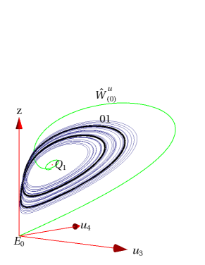
(a)     (b)

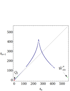
Figure 4: (a) Invariant image of complex Lorenz flow, figure 1, projected onto the invariant polynomials basis (32). Note the unstable manifold connection from the equilibrium $\mathrm{E}_{0}$ at the origin to the strange attractor controlled by the rotation around the reduced state space image of relative equilibrium $\mathrm{Q}_{1}$; as for the Lorenz flow [1], the natural measure close to $\mathrm{E}_{0}$ is vanishingly small but non-zero. (b) The return map for the Poincaré surface of section $u_{1}=u_{4}$ for the complex Lorenz equations projected on invariant polynomials (32). The return map coordinate is the Euclidean length (36) along the Poincaré section of the unstable manifold of $\mathrm{Q}_{1}$.

Vladimirov, Toronov and Derbov [49] use a different invariant polynomial basis to study bounding manifolds of the symmetry reduced complex Lorenz flow and its homoclinic bifurcations.

Application of the chain rule (31) brings the equivariant complex Lorenz equations (13) to the invariant form (32):

$$\dot{u}_{1} = 2\,\sigma\,(u_{4}-u_{1})\,,$$

$$\dot{u}_{2} = -2\left(\,u_{2}-\rho_{2}\,u_{3}-\,(\rho_{1}-u_{5})\,u_{4}\right)\,,$$

$$\dot{u}_{3} = -(\sigma\,+1)\,u_{3}+\rho_{2}\,u_{1}+e\,u_{4}\,,$$ (34)

$$\dot{u}_{4} = -(\sigma\,+1)\,u_{4}+\,(\rho_{1}-u_{5})\,u_{1}+\sigma\,u_{2}-e\,u_{3}\,,$$

$$\dot{u}_{5} = u_{4}-b\,u_{5}\,.$$

As far as visualization goes, we need neither construct the invariant equations (34) nor integrate them. It suffices to integrate the original, unreduced flow of Figure 1, but plot the solution in the image space, i.e., the invariant, Hilbert polynomial coordinates $u_{i}$, as in figure 4 (a). A minor drawback of the Hilbert polynomial basis projections is that the folding mechanism is harder to view since the dynamics is squeezed near the $z$-axis.

5.2 Symmetry reduced return map

Successive trajectory intersections with a Poincaré section, a $(d-1)$-dimensional manifold or a set of manifolds $\cal P$ embedded in the $d$-dimensional state space ${\cal M}$, define the Poincaré return map $P({x})$, a $(d-1)$-dimensional map of form

$$x^{\prime}=P({x})={f^{\tau(x)}(x)}\,,\qquad x^{\prime},x\in\cal P\,.$$ (35)

Here the first return function $\tau(x)$, sometimes referred to as the ceiling function, is the time of flight to the next Poincaré section for a trajectory starting at $x$. A good choice of the Poincaré section manifold $\cal P$ in high-dimensional ($d>3$) flows is basically a dark art. We chose a Poincaré section which contains the $z$-axis and the relative equilibrium, here defined by the condition $u_{1}=u_{4}$. Even though in the complex Lorenz equations case we could use one of the $u_{i}$’s as a coordinate to construct a return map, for high dimensional flows a dynamically intrinsic parametrization is the only option. Following ref. [6], we construct the first return map of figure 4 (b) using as a coordinate the Euclidean length along the intersection of the unstable manifold of $\mathrm{Q}_{1}$ within the Poincaré surface of section, measured from $\mathrm{Q}_{1}$.

We begin by sprinkling evenly spaced points $\{x^{(1)},x^{(2)},\cdots,x^{(N-1)}\}$ between the relative equilibrium point $x_{\mathrm{Q}_{1}}=x^{(0)}$ and the point $x=x^{(N)}$, along the $1d$ intersection of Poincaré section and unstable manifold continuation $x^{(k)}\in\hat{W}^{u}_{(1)}$ of the unstable ${\bf\hat{e}}^{(1)}$ eigenplane (we shall omit the eigendirection label ₍₁₎ in what follows). Then the arclength in Euclidean metric from the relative equilibrium point $x_{\mathrm{Q}_{1}}=x^{(0)}$ to $x=x^{(N)}$ is given by

$$s=\lim_{N\to\infty}\sqrt{\sum_{k=1}^{N}\left(dx^{(k)}\right)^{2}}\,.$$ (36)

By definition $f^{\tau(x)}(x)\in\hat{W}^{u}_{(j)}$, so $f^{t}(x)$ induces a $1d$ map $s(s_{0},\tau)=s(f^{\tau({x_{0}})}({x_{0}}))$.

Turning points are points on the unstable manifold for which the local unstable manifold curvature diverges for forward iterates of the map, i.e., points at which the manifold folds back onto itself arbitrarily sharply. The $1d$ curve $\hat{W}^{u}_{(1)}$ starts out linear at $x_{\mathrm{Q}_{1}}$, then gently curves until it folds back sharply at the ‘turning point’ along a possible heteroclinic connection to $\mathrm{E}_{0}$, and then nearly retraces itself.

The trick is to figure out a good base segment to the nearest turning point $L=[0,s_{b}]$, and after the foldback assign to $s(x,t)>s_{b}$ the nearest point $s$ on the base segment. Since here the stable manifold contraction is strong, the 2nd coordinate connecting $s(x,t)\to s$ can be neglected.

Armed with this intrinsic curvilinear coordinate parametrization, we are now in a position to construct a 1-dimensional model of the dynamics on the non–wandering set. If $\hat{x}_{n}$ is the $n$th Poincaré section of a trajectory in neighborhood of $x_{q}$, and $s_{n}$ is the corresponding curvilinear coordinate, then $s_{n+1}=f^{\tau_{n}}(s_{n})$ models the full state space dynamics $\hat{x}_{n}\to\hat{x}_{n+1}$. We approximate $f(s_{n})$ by a smooth, continuous 1-dimensional map $f:L_{q}\to L_{q}$ by taking $\hat{x}_{n}\in L_{q}$, and assigning to $\hat{x}_{n+1}$ the nearest base segment point $s_{n+1}=s(\hat{x}_{n+1})$. Thanks to the extreme contraction rate (18), the return map turns out to be unimodal for all practical purposes, so binary symbolic dynamics are easily constructed and admissible periodic orbits of the map up to desired length can be systematically obtained. A multiple shooting routine [5] can then be used to determine the corresponding relative periodic orbits of the complex Lorenz equations to machine precision.

6 The method of moving frames

The method of moving frames, introduced by G. Darboux and systematized by É. Cartan [50], is interpreted by Fels and Olver [51, 52] as a map from a $d$-dimensional manifold to a $N$-dimensional Lie group acting on it. Moving frames are then used to compute $d-N$ functionally independent fundamental invariants for general group actions in relation to general equivalence problems. ‘Fundamental’ here means that they can be used to generate all other invariants, and, in particular, they serve to distinguish group orbits in an open neighborhood of the slice point, i.e., two points lie on the same group orbit if and only if all fundamental invariants agree. For an introduction to the method we recommend Olver’s pedagogical monograph [26]. Here we emphasize the application of the method to dynamical symmetry reduction, and focus in particular on groups acting on spaces with the structure of a direct sum of irreducible subspaces, an application which is not to our knowledge explored in the literature. We are not concerned with the explicit determination of the fundamental invariants as in ref. [51, 52], except for illustrative purposes; instead we focus on implementation of a moving frame transformation as a numerically fast and efficient linear map of the full state space dynamics onto its desymmetrized, reduced state space projection.

The main idea behind method of moving frames is that we can, at least locally, map each point along any solution $x(\tau)$ to a unique representative $\overline{x}(\tau)$ of the associated group orbit equivalence class, by a suitable rotation

$$x(\tau)=g(\tau)\,\overline{x}(\tau)\,.$$ (37)

Equivariance implies the two points are equivalent. In the method of moving frames the reduced state space representative $\overline{x}$ of a group orbit equivalence class is picked by slicing across the group orbits by a fixed manifold.

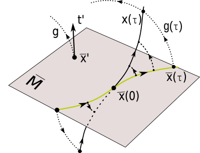
(a)     (b)

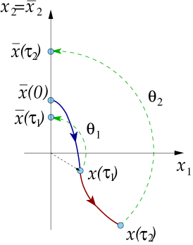
Figure 5: (a) Slice $\overline{\cal M}$ is a hyperplane (38) passing through the slice-fixing point ${\overline{x}^{\prime}}$, and normal to the group tangent $t^{\prime}$ at ${\overline{x}^{\prime}}$. It intersects all group orbits (indicated by dotted lines here) in an open neighborhood of ${\overline{x}^{\prime}}$. The full state space trajectory $x(\tau)$ and the reduced state space trajectory $\overline{x}(\tau)$ belong to the same group orbit ${\cal M}_{x(\tau)}$ and are equivalent up to a group rotation $g(\tau)$.  (b) The method of moving frames for a flow $\textrm{SO}(2)$-equivariant under (16) with slice through ${\overline{x}^{\prime}}=(0,1,0,0,0)$, group tangent $t^{\prime}=(-1,0,0,0,0)$. The orientation condition restricts the slice to half-hyperplane $\overline{x}_{1}=0,\;\overline{x}_{2}\geq 0$. A trajectory started on the slice at $\overline{x}(0)$ evolves to a state space point with a non-zero $x_{1}(\tau_{1})$. Compute angle ${\bf\theta}_{1}$ through slice condition (39). Rotate $x(\tau_{1})$ counter-clockwise by ${\bf\theta}_{1}$ to $\overline{x}(\tau_{1})=g({\bf\theta}_{1})\,x(\tau_{1})$, so that the equivalent point on the circle lies on the slice, $\overline{x}_{1}(\tau_{1})=0$. Repeat for all sample points $x(\tau_{i})$ along the trajectory.

In the following it will be useful to introduce the notion of a slice, an $(d-N)$-dimensional submanifold $\overline{\cal M}\subset{\cal M}$ such that $\overline{\cal M}$ intersects all group orbits in an open neighborhood of ${\overline{x}^{\prime}}\in\overline{\cal M}$ transversally and at most once. In other words, slice is the analogue of a Poincaré section, but for group orbits. As is the case for the dynamical Poincaré sections, in general a single slice does not suffice to intersect all group orbits of points in ${\cal M}$. One can construct a local slice passing through any point $x\in{\cal M}$ if the group orbits of $G$ have the same dimension, i.e. they are away from fixed-point subspaces of continuous subgroups of $G$, see ref. [52] for details.

The simplest slice condition defines a linear slice as a $(d\!-\!N)$-dimensional hyperplane $\overline{\cal M}$ normal to the $N$ group rotation tangents $t^{\prime}_{a}$ at point ${\overline{x}^{\prime}}$, see figure 5:

$$(\overline{x}-{\overline{x}^{\prime}})^{T}t^{\prime}_{a}=0\,,\qquad t^{\prime}_{a}=t_{a}({\overline{x}^{\prime}})=\mathbf{T}_{a}\,{\overline{x}^{\prime}}\,,\qquad a=1,2,\cdots,N\,.$$ (38)

As ${\overline{x}^{\prime}}^{T}t^{\prime}_{a}=0$ by the antisymmetry of $\mathbf{T}_{a}$, the slice condition (38) fixes ${\bf\theta}$ for a given $x$ by orthogonality,

$$0=\overline{x}^{T}t^{\prime}_{a}=x^{T}g({\bf\theta})^{T}t^{\prime}_{a}\,,$$ (39)

where $g^{T}$ denotes the transpose of $g$. A group orbit will in general intersect a slice more than once (for example in the case of $\textrm{SO}(2)$, two $\pi$-separated points), so we need to impose further conditions on the slice, in the form of either inequalities or orientation conditions, so as to ensure unique intersection. These restrictions are rather arbitrary, the only requirement being that $\overline{\cal M}$ remains a connected manifold. We illustrate this point for the complex Lorenz flow example in sect. 6.1.

For group orbits intersected by a slice, we can identify the unique group element $g=g(x)$ that rotates $x$ into the slice, $gx=\overline{x}\in\overline{\cal M}$. The map that associates to a state space point $x$ a Lie group action $g(x)$ is called a moving frame. The method of moving frames can be thought of as a change of variables $\overline{x}=g^{-1}(x)\,x\,,$ to a frame of reference for which the slice-fixing condition (39) is identically satisfied–hence the name ‘moving frame.’

The method of moving frames is a post-processing method; trajectories are computed in the full state space, then rotated into the slice whenever desired, with the slice condition easily implemented. The slice group tangent $t^{\prime}_{\ }$  is a given vector, and rotation parameters ${\bf\theta}$ are determined numerically, by a Newton method, through the slice condition (39). For given $\theta$, $g({\bf\theta})\,x$ is another vector, linear in $x$.

A slice can be identified with ${\cal M}/G$ in an open neighborhood of ${\overline{x}^{\prime}}$. As is the case for the dynamical Poincaré sections, a single slice does not suffice to reduce ${\cal M}\to{\cal M}/G$ globally as one cannot expect the group orbit of any point in ${\cal M}$ to intersect a given slice.

How does one pick a slice point ${\overline{x}^{\prime}}$? A generic point ${\overline{x}^{\prime}}$ not in an invariant subspace (on the $z$ axis of the complex Lorenz equations, for example) should suffice to fix a slice. The rules of thumb are much like the ones for picking Poincaré sections. The intuitive idea is perhaps best visualized in the context of fluid flows. Suppose the flow exhibits an unstable coherent structure that is frequently visited at different spatial dispositions. One can fit a ‘template’ to one recurrence of such structure, and describe other recurrences as its translations. A well-chosen slice point belongs to equivalence class that is dynamically important in this way (i.e., a group orbit). We discuss, in the context of our complex Lorenz equations example, several slice fixing choices in sects. 6.2 and 6.3.

A historical note. For the definition of slice see, for example, Chossat and Lauterbach [45]. Slices tend to be discussed in contexts much more difficult than our application - symplectic groups, sections in absence of global charts, non-compact Lie groups. We follow ref. [53] in referring to a local group-orbit section as a slice. The usage goes back at least to Palais [54] in 1961 and Mastow [55] in 1957. Some [52, 27] refer to global group-orbit sections as cross-sections, a term that we would rather avoid, as it has an honest, well-established meaning in physics. Guillemin and Sternberg [56] define the cross-section, but emphasize that finding it is very rare: “existence of a global section is a very stringent condition on a group action. The notion of slice is weaker but has a much broader range of existence.”

6.1 An example: Moving frame for complex Lorenz equations

In case of the complex Lorenz equations we can, due to equivariance, rotate any slice fixing point in (39) so that we have ${\overline{x}^{\prime}_{1}}=0$. As only the group tangent direction matters, a slice that goes through point (0, $\overline{x}^{\prime}_{2}$, $\overline{y}^{\prime}_{1}$,  $\overline{y}^{\prime}_{2}$, $\overline{z}^{\prime}$) is equivalent to (0, 1, $\overline{y}^{\prime}_{1}$/$\overline{x}^{\prime}_{2}$,  $\overline{y}^{\prime}_{2}$/$\overline{x}^{\prime}_{2}$, 0), so we can specify the most general slice fixing point for the complex Lorenz equations by two numbers,

$${\overline{x}^{\prime}}=(0,\,1,\,{\overline{y}^{\prime}_{1}},\,{\overline{y}^{\prime}_{2}},\,0)\,.$$ (40)

The group orbit tangent then becomes $t^{\prime}=(-1,\,0,\,-{\overline{y}^{\prime}_{2}},\,{\overline{y}^{\prime}_{1}},\,0)$ and slice condition (39) leads to

$$\theta=\tan^{-1}\frac{x_{1}+{\overline{y}^{\prime}_{2}}y_{1}-{\overline{y}^{\prime}_{1}}y_{2}}{x_{2}+{\overline{y}^{\prime}_{1}}y_{1}+{\overline{y}^{\prime}_{2}}y_{2}}\,.$$ (41)

To ensure a unique intersection with the slice, we have to further restrict $\overline{\cal M}$ by choosing a representative out of the two group orbit points that intersect the slice. One can impose an orientation condition, for example choosing the point that is at minimum distance from ${\overline{x}^{\prime}}$, or one can define the inverse tangent function $\tan^{-1}({b}/{a})$ so that it distinguishes quadrants in the $(a,b)$ plane. Either condition works equally well.

We observe that (41) is undefined when

$$x_{1}+{\overline{y}^{\prime}_{2}}y_{1}-{\overline{y}^{\prime}_{1}}y_{2} =0\,,$$ (42a)

$$x_{2}+{\overline{y}^{\prime}_{1}}y_{1}+{\overline{y}^{\prime}_{2}}y_{2} =0\,,$$ (42b)

are both satisfied. We will refer to this $3$-dimensional linear subspace as the singular set of the moving frame associated with (41). Condition (42a) implies that point $x$ is already on the slice, $x^{T}{\overline{x}^{\prime}}=0$. Condition (42b) implies that the group tangent at point $x$ is perpendicular to group tangent at slice fixing point, $t{}(x)^{T}t^{\prime}=-x^{T}{\overline{x}^{\prime}}=0$. The problem lies in the fact that the limit of (42) as we approach the singular set does not exist. For instance, consider points for which (42b) holds; as we approach the singularity with positive values of the numerator in (41) we have $\theta=\pi/2$, while for negative values $\theta=-\pi/2$. A $\pi$-jump occurs as we cross the singular set. In general such crossings are expected to occur, since the singular set is not flow invariant. Even worse, the singularity distorts the way trajectories are mapped onto the slice, even if they merely approach it rather than cross it, as we will see in the next two examples.

6.2 Irreducible subspace slice and explicit invariants

We now show how a particular choice of the slice point enables us to express the transformation to invariant variables in a simple analytic form. Place the slice point in one of the linearly irreducible subspaces of $\textrm{SO}(2)$ action (16), for instance ${\overline{x}^{\prime}}=(0,-1,0,0,0)$. The group-tangent at the slice point is then $t^{\prime}=(1,0,0,0,0)$ and the slice fixing condition is

$$\overline{x}_{1}=x_{1}\cos{\bf\theta}-x_{2}\sin{\bf\theta}=0\,.$$ (43)

The orientation condition restricts the slice to half-hyperplane $\overline{x}_{1}=0,\;\overline{x}_{2}\geq 0$. Solving (43) for the polar angle ${\bf\theta}$ in $(x_{1},x_{2})$ we get

$${\bf\theta}=\tan^{-1}({x_{1}}/{x_{2}})\,.$$ (44)

The transformation that rotates $x$ counter-clockwise by ${\bf\theta}$ to $\overline{x}=g({\bf\theta})\,x$ onto the slice is found by inserting (44) into the expression for the action of $\textrm{SO}(2)$ on $x$,

$$\overline{x}_{1} = x_{1}\cos{\bf\theta}-x_{2}\sin{\bf\theta}\,,\quad\overline{x}_{2}=x_{1}\sin{\bf\theta}+x_{2}\cos{\bf\theta}$$ (45)

$$\overline{y}_{1} = y_{1}\cos{\bf\theta}-y_{2}\sin{\bf\theta}\,,\quad\overline{y}_{2}=y_{1}\sin{\bf\theta}+y_{2}\cos{\bf\theta}$$

yielding the transformations in analytic form:

$$\overline{x}_{2} = r_{1}\,=\,\sqrt{x_{1}^{2}+x_{2}^{2}}\,,\qquad\overline{z}\,=\,z$$

$$\overline{y}_{1} = {(x_{2}y_{1}-x_{1}y_{2})}/{r_{1}}\,,\quad\overline{y}_{2}\,=\,{(x_{1}y_{1}+x_{2}y_{2})}/{r_{1}}\,.$$ (46)

This transformation rotates point $x$ into the slice point $\overline{x}$. Alternatively, the transformation can be viewed as providing invariant variables on which to project dynamics, as we did in Hilbert basis case. Note the relation to the invariant polynomials (32), and observe that as the rotational degree of freedom has been explicitly used, the method of moving frames requires no syzygies. Analytical determination of invariant variables through moving frame transformations and particular slice conditions can be carried out systematically for general group representations [51], but for reasons explained in sect. 6.3, we shall not take this path here.

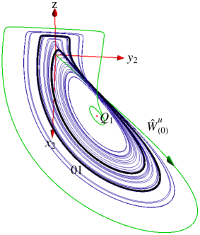
(a)     (b)

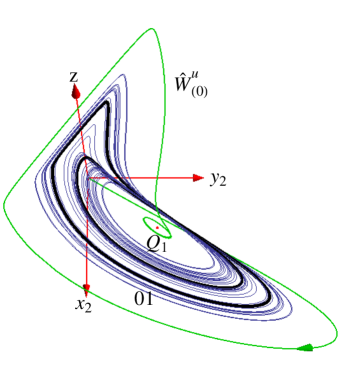
Figure 6: State space portrait of complex Lorenz flow in reduced state space, projected on the slice, taking as the slice fixing point ${\overline{x}^{\prime}}$ (a) the irreducible subspace slice condition (43), (b) the relative equilibrium $x_{\mathrm{Q}_{1}}$.

As in sect. 6.1, note that the invariants are not well defined in the $x_{1},\,x_{2}\to 0$ limit. Using $x=r_{1}\,e^{i\phi_{1}}\,,\,y=r_{2}\,e^{i\phi_{2}}$ we can write

$$\overline{x}_{2} = r_{1}\,,\qquad\overline{y}_{1}\,=\,r_{2}\sin(\phi_{1}-\phi_{2})$$

$$\overline{y}_{2} = r_{2}\cos(\phi_{1}-\phi_{2})\,,\qquad\overline{z}\,=\,z\,.$$ (47)

For any given $y$ (therefore also for given $\phi_{2}$), the limit of $\overline{y}$ for $x\rightarrow 0$ does not exist, as the above expression depends on the direction in the complex $x$-plane along which we approach zero.

From a different perspective, we may redefine the slice so that $x_{1}=x_{2}=0$ is excluded, that is by $\overline{x}_{1}=0,\;\overline{x}_{2}>0$. Then we may say that group orbits of points in the $x_{1}=x_{2}=0$ subspace fail to intersect the slice. In figure 6 (a) this becomes apparent by the trajectories in reduced space being stretched as they come closer to $x_{1}=x_{2}=0$ subspace, where transverse intersection would eventually fail.

It is instructive to rewrite the complex Lorenz equations (12) in terms of the invariant variables (46). This is achieved by using the chain rule (31) and expressing the result in terms of variables (46). The moving frames symmetry-reduced complex Lorenz equations are a 4-dimensional ODE system

$$\dot{\overline{x}}_{2} = -\sigma\,(\overline{x}_{2}-\overline{y}_{2})\,,\quad\dot{\overline{y}}_{1}\,=\,-\overline{y}_{1}+\rho_{2}\overline{x}_{2}-\left(e+{\sigma\,\overline{y}_{1}}/{\overline{x}_{2}}\right)\overline{y}_{2}$$

$$\dot{\overline{y}}_{2} = -\overline{y}_{2}+(\rho_{1}-z)\,\overline{x}_{2}+\left(e+{\sigma\,\overline{y}_{1}}/{\overline{x}_{2}}\right)\overline{y}_{1}\,,\quad\dot{z}\;\,=\,-b\,z+\overline{x}_{2}\overline{y}_{2}\,.$$ (48)

Note the singularity as $\overline{x}_{2}=r_{1}\rightarrow 0$.

The projections in figure 6 help us understand the topology of the dynamics but also present large discontinuous jumps. Note that the invariants (46) are related to the invariant polynomials (32) by division by $\sqrt{x_{1}^{2}+x_{2}^{2}}$. This is the reason we get a clearer visualization of the dynamics than with invariant polynomials: All invariants scale as the original coordinates. At the same time division by $\sqrt{x_{1}^{2}+x_{2}^{2}}$ causes the jumps in the $\overline{y}$ components whenever the magnitude of $x$ comes close to zero.

So what does this imply for the ultimate goal of this paper, “Continuous symmetry reduction and return maps for higher-dimensional flows?” In this example there is no problem. It is obvious by inspection of figure 6 that one can chose a Poincaré section away from the singular set. Repeating the construction of sect. 5.2 results in a return map very much like the one of figure 4 (b), with the same admissible orbits, so there is no need to plot further return maps for various choices of slices.

6.3 Complex Lorenz equations: the general linear slice

The irreducible subspace slice condition (43) yields the invariant variables (46) in explicit, analytic form. As explained in sect. 6.1, the method of moving frames also introduces artificial singularities in reduced state space, the location of which depend on the choice of slice point, and one might suspect that the singularities encountered by the strange attractor are due to very special choice of the slice fixing condition. How does a general choice of the slice fixing point affect the singular set? In this setting it is no longer convenient to explicitly write out transformations to invariant variables as we did in sect. 6; we will implement the moving frame map numerically, mapping computed trajectories to the slice. Even though the analytical computation of invariants by the method of moving frames can be implemented by computer algebra [20] for system dimensions of the order of $100$, it is both computationally prohibitive and utterly unnecessary for symmetry reduction of very high dimensional flows of order $100,000$ required for fully resolved $3$-D fluid simulations [57].

Since $\mathrm{Q}_{1}$ organizes reduced space dynamics around it, but also sets the scale of angular velocity of symmetry induced rotations in the system, we find it natural to choose slice-fixing point (40) computed from group orbit of the relative equilibrium $x_{\mathrm{Q}_{1}}$, given in (28) for the parameter values used here. We can use (41) to compute $\theta$ for any point $x$, but keeping up with the numerical approach of this section, we use a Newton’s method. As an initial guess we use the angle from previous point along the trajectory, while for the first point we choose among the two possible solutions by demanding that the rotation brings the point to a minimum distance from $\overline{x}^{\prime}$. Projections of complex Lorenz flow to the slice defined in this manner are shown in figure 6 (b). This projection of the strange attractor also clearly exhibits the moving frame angle $\pi$-jumps. Figure 7(a) shows the projection of singular set in $3$-dimensions $(x_{1},x_{2},y_{1})$; the attractor collides with the singular set head on.

The linear relation (42b) and figure 7 suggest that we can manipulate the singular set so that the attractor avoids the singularity by increasing the ratio ${\overline{y}^{\prime}_{2}}/{\overline{y}^{\prime}_{1}}$. Choosing the slice fixing point as ${\overline{x}^{\prime}}=x_{\mathrm{Q}_{1}}+(5,0,0,0,0)$ we can ‘tilt’ the singular set so that trajectories approach it in a smoother manner, see figure 7 (b).

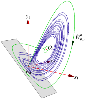
(a)     (b)

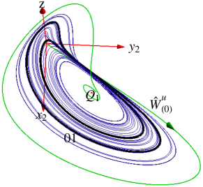
Figure 7: State space portraits of complex Lorenz flow in reduced state space. We use a moving frame map to a slice fixed by point (a) ${\overline{x}^{\prime}}=x_{\mathrm{Q}_{1}}$, with the gray plane indicating the singular set. (b) ${\overline{x}^{\prime}}=x_{\mathrm{Q}_{1}}+(5,0,0,0,0)$. Compare with figure 6 (b).

For more pointers on how to pick good slices and combine them with well-chosen Poincaré sections, the reader is referred to ref. [20].

7 Differential formulation: the method of slices

Instead of post-processing a full state space trajectory, we can proceed as follows: Split up the integration into a sequence of short time steps, each followed by a rotation of the final point such that the next segment’s initial point is in the slice fixed by a point ${\overline{x}^{\prime}}$. In the infinitesimal steps limit this leads to the method of slices, a differential form of the method of moving frames for which the trajectory never leaves the reduced state space.

Consider an $N$-dimensional Lie group $G$ acting on $d$-dimensional space and which, at least locally near ${\overline{x}^{\prime}}$, has $N$-dimensional orbits. For points that can be mapped by a moving frame to slice through ${\overline{x}^{\prime}}$ we can write, using decomposition (37), the full state space trajectory as $x(\tau)=g(\tau)\,\overline{x}(\tau)$, where the $(d\!-\!N)$-dimensional reduced state space trajectory $\overline{x}(\tau)$ is to be fixed by some condition, and $g(\tau)$ is then the corresponding group action on the $N$-dimensional group manifold that rotates $\overline{x}$ into $x$ at time $\tau$. The time derivative is $\dot{x}=v(g\overline{x})=\dot{g}\overline{x}+gu$, with the reduced state space velocity field given by $u={d\overline{x}}/{d\tau}$. Rewriting this as $u=g^{-1}v(g\,\overline{x})-g^{-1}\dot{g}\,\overline{x}$ and using the equivariance condition (3) leads to

$$u=v-g^{-1}\dot{g}\,\overline{x}\,.$$

The Lie group element (4) and its time derivative describe the group tangent flow

$$g^{-1}\dot{g}=g^{-1}\frac{d~{}}{d\tau}e^{{\bf\theta}\cdot\mathbf{T}}=\dot{{\bf\theta}}\cdot\mathbf{T}\,.$$

This is the group tangent velocity $g^{-1}\dot{g}\,\overline{x}=\dot{{\bf\theta}}\cdot t(\overline{x})$ evaluated at the point $\overline{x}$, i.e., with ${g}=1$, see figure 5 (a). The flow in the $(d\!-\!N)$ directions transverse to the group flow is now obtained by subtracting the flow along the group tangent direction,

$$u(\overline{x})=v(\overline{x})-\dot{{\bf\theta}}(\overline{x})\cdot t(\overline{x})\,,\qquad u={d\overline{x}}/{d\tau}\,,$$ (49)

for any factorization of the flow of form $x(\tau)=g(\tau)\,\overline{x}(\tau)$. To integrate these equations we first have to fix a particular flow factorization by imposing conditions on $\overline{x}(\tau)$, and then integrate phases ${\bf\theta}(\tau)$ on a given reduced state space trajectory $\overline{x}(\tau)$.

Here we shall demand that the reduced state space is confined to a linear hyperplane slice. Substituting (49) into the time derivative of the fixed slice condition (39),

$$u(\overline{x})^{T}t^{\prime}_{a}=v(\overline{x})^{T}t^{\prime}_{a}-\dot{{\bf\theta}}_{a}\cdot t(\overline{x})^{T}t^{\prime}_{a}=0\,,$$

yields the equation for the group phases flow $\dot{{\bf\theta}}$ for the slice fixed by $\overline{x}^{\prime}$, together with the reduced state space $\overline{\cal M}$ flow $u(\overline{x})$:

$$\dot{{\bf\theta}}_{a}(\overline{x}) = \frac{v(\overline{x})^{T}t^{\prime}_{a}}{t(\overline{x})^{T}\cdot t^{\prime}}$$ (50)

$$u(\overline{x}) = v(\overline{x})\,-\,\dot{{\bf\theta}}(\overline{x})\cdot t(\overline{x})\,,\qquad\quad\overline{x}\in\overline{\cal M}\,.$$ (51)

Each group orbit ${\cal M}_{x}=\{g\,x\,|\,g\in G\}$ is an equivalence class; the method of slices represents the class by its single slice intersection point $\overline{x}$. By construction $u^{T}t^{\prime}_{a}=0$, and the motion stays in the $(d\!-\!N)$-dimensional slice. We have thus replaced the original dynamical system $\{{\cal M},f\}$ by a reduced system $\{\overline{\cal M},\bar{f}\}$.

These equations are easily integrated (provided some care is taken about how the trajectories cross the singular set), and given the same slice-fixing conditions, the integrations reproduce the plots obtained by the method of moving frames, such as figure 6.

For example, consider the complex Lorenz equations slice condition of sect. 6.2: $x_{1}=0,\;x_{2}>0$. The reduced state space equations are given by

$$u(\overline{x})=v(\overline{x})-\frac{v_{1}}{\overline{x}_{2}}t(\overline{x})\,.$$ (52)

Substitution of the complex Lorenz equations equations recovers (48), obtained by the method of moving frames. The integration of (48) recovers the strange attractor in figure 6 (a), obtained by simulation in the full state space, followed by moving frame rotation into the slice.

In pattern recognition and ‘template fitting’ settings, (50) is called the reconstruction equation. We have already encountered it in our polar coordinates exercise (25). Integrated together, the reduced state space trajectory (51), the integrated phase (50), and $g(\tau)=\exp[{\bf\theta}(\tau)\cdot\mathbf{T}]$ reconstruct the full state space trajectory $x(\tau)=g(\tau)\,\overline{x}(\tau)$ from the reduced state space  trajectory $\overline{x}(\tau)$, so no information about the flow is lost in the process of symmetry reduction.

The denominator in (50) vanishes and the phase velocity $\dot{{\bf\theta}}(\overline{x})$ diverges whenever the direction of group action on the reduced state space point is perpendicular to the direction of group action on the slice point ${\overline{x}^{\prime}}$. Therefore the method of slices has the same singular set as its post-processing variant, the method of moving frames: the intersection of the slice with the set of points with group tangent perpendicular to $t^{\prime}$.

A historical note. The basic idea of the method of slices is intuitive and frequently reinvented, often under a different name; for example, it is stated without attribution as problem 1. of Sect. 6.2 of Arnol’d Ordinary Differential Equations [58]. The factorization (37) is stated on p. 31 of Anosov and Arnol’d [59], who note, without further elaboration, that in the vicinity of a point that is not fixed by the group one can reduce the order of a system of differential equations by the dimension of the group. Fiedler, in the influential 1995 talk at the Newton Institute, and Fiedler, Sandstede, Wulff, Turaev and Scheel [60, 61, 62, 63] treat Euclidean symmetry bifurcations in the context of spiral wave formation. The central idea is to utilize the semidirect product structure of the Euclidean group $E(2)$ to transform the flow into a ‘skew product’ form, with a part orthogonal to the group orbit, and the other part within it, as in (51). They refer to a linear slice $\overline{\cal M}$ near a relative equilibrium as a Palais slice, with Palais coordinates. As the choice of the slice is arbitrary, these coordinates are not unique. According to these authors, the skew product flow was first written down by Mielke [64], in the context of buckling in elasticity theory. However, this decomposition is no doubt much older. For example, it was used by Krupa [28, 45] in his local slice study of bifurcations of relative equilibria. Biktashev, Holden, and Nikolaev [65] cite Anosov and Arnol’d [59] for the ‘well-known’ factorization (37) and write down the slice flow equations (51). Haller and Mezić [66] reduce symmetries of three-dimensional volume preserving flows and reinvent method of moving frames, under the name ‘orbit projection map.’ There is extensive literature on reduction of symplectic manifolds with symmetry; the Marsden and Weinstein 1974 article [67] is an important early reference. Then there are studies of the reduced phase spaces for vortices moving on a sphere such as ref. [68], and many, many others.

Neither Fiedler et al. [60] nor Biktashev et al. [65] implemented their methods numerically. That was done by Rowley and Marsden for the Kuramoto-Sivashinsky [53] and the Burgers [69] equations, and Beyn and Thümmler [70, 71] for a number of reaction-diffusion systems, described by parabolic partial differential equations on unbounded domains. We recommend the Barkley paper [72] for a clear explanation of how the Euclidean symmetry leads to spirals, and the Beyn and Thümmler paper [70] for inspirational concrete examples of how freezing/slicing simplifies the dynamics of rotational, traveling and spiraling relative equilibria.

Beyn and Thümmler write the solution as a composition of the action of a time dependent group element $g(\tau)$ with a ‘frozen,’ in-slice solution $\hat{u}(\tau)$ (37). In their nomenclature, making a relative equilibrium stationary by going to a co-moving frame is ‘freezing’ the traveling wave, and the imposition of the phase condition (i.e., slice condition (38)) is the ‘freezing ansatz.’ They find it more convenient to make use of the equivariance by extending the state space rather than reducing it, by adding an additional parameter and a phase condition. The freezing ansatz [70] is identical to the Rowley and Marsden [69] and our slicing, except that freezing is formulated as an additional constraint, just as when we compute periodic orbits of ODEs we add Poincaré section as an additional constraint, i.e., increase the dimensionality of the problem by 1 for every continuous symmetry.

Our derivation of method of slices follows most closely Rowley and Marsden [69] who in the pattern recognition setting refer to the slice point as a template, and call (50) the reconstruction equation [73]. They also describe the ‘method of connections’ (called ‘orthogonality of time and group orbit at successive times’ in ref. [70]), for which the reconstruction equation (50) denominator is $t(\overline{x})^{T}\cdot t(\overline{x})$ and thus nonvanishing as long as the action of the group is regular. This avoids the spurious slice singularities, but it is not clear what the method of connections buys us otherwise. It does not reduce the dimensionality of the state space, and it accrues geometric phases which prevent relative periodic orbits from closing into periodic orbits. Geometric phase in laser equations, including complex Lorenz equations, has been studied in ref. [74, 75, 76, 77, 78].

One would think that with all the literature on desymetrization the case is shut and closed, but not so. Applied mathematicians are inordinately fond of bifurcations, and almost all of the previous work focuses on equilibria, relative equilibria (traveling waves), and their bifurcations, and for these problems a single slice works well. Only when one tries to describe the totality of chaotic orbits does the non-global nature of slices become a serious nuisance.

8 Discussion and conclusions

We have presented two approaches to continuous symmetry reduction of higher-dimensional flows and illustrated them with reductions of the complex Lorenz system, a 5-dimensional dissipative flow with rotational symmetry. In either approach numerical computations can be performed in the original, full state-space representation, and then the solutions can be projected onto the symmetry-reduced state space.

In the Hilbert polynomial basis approach, one transforms the equivariant state space coordinates into invariant coordinates by a nonlinear coordinate transformation

$$\{x_{1},x_{2},\cdots,x_{d}\}\to\{u_{1},u_{2},\cdots,u_{m}\}\,,$$

and studies the invariant image of dynamics rewritten in terms of invariant coordinates. These invariant polynomial bases can be algorithmically determined for both Hamiltonian and dissipative systems. Our goal is to reduce symmetries of fully-resolved simulations of PDEs, with state space dimensions of the order of a few tens to few hundreds (for Kuramoto-Sivashinsky flow), and well into the tens or hundreds of thousands (for pipe and plane Couette flows). Unfortunately, the computational cost of polynomial basis algorithms is at present prohibitive for state space dimensions larger than ten, so the invariant polynomial basis approach is not a feasible option. We have discussed it here solely for illustrative purposes.

In the method of moving frames (or its continuous time, differential version, the method of slices), one fixes a local slice $(\overline{x}-{\overline{x}^{\prime}})^{T}t^{\prime}=0$, a hyperplane normal to the group tangent $t^{\prime}$ that cuts across group orbits in the neighborhood of the slice-fixing point ${\overline{x}^{\prime}}$. The state space is sliced locally in such a way that each group orbit of symmetry-equivalent points is represented by a single point, with the symmetry-reduced dynamics in the reduced state space ${\cal M}/G$ given by (51):

$$u=v-\dot{{\bf\theta}}\cdot t\,,\qquad\dot{{\bf\theta}}=(v\cdot t^{\prime})/(t\cdot t^{\prime})\,.$$

The method of moving frames turns out to be an efficient method for reducing the flow to a symmetry-invariant reduced state space, suited to reduction of even very high-dimensional dissipative flows to local return maps: one runs the dynamics in the full state space and post-processes the trajectory by the method of moving frames. Importantly, from a numerical point of view, there is no need to actually recast the dynamics in the new coordinates or write new code. Either approach can be used as a visualization tool, with all computations carried out in the original coordinates, and then, when done, projecting the solutions onto the symmetry reduced state space by post-processing the data. In contrast to co-moving frames local to each traveling solution, restricting the dynamics to a slice renders all relative equilibria stationary in the same set of coordinates.

An inconvenience inherent in the linear slices formulation is that they are local, and the reduced flow encounters singularities in subsets of the reduced state space, with the reduced trajectory exhibiting large, slice-induced jumps. This singular set is introduced by and depends on the slice-fixing condition. We have shown, in the $5$-dimensional complex Lorenz equations example, that the location of the singular set can be manipulated by judicious choice of the slice fixing point, and geometrical information about the dynamics can be extracted by constructing a return map through a Poincaré section that does not intersect the singular set. The trick is to construct a good set of symmetry invariant Poincaré sections, and that is a dark art for systems of dimension higher than three, with or without a symmetry. In higher-dimensional flows, with more involved symmetry group actions and larger sets of stationary solutions, where a single slice and Poincaré section will not suffice, we can still expect to cover the reduced state space with multiple slices, obtaining a set of discrete maps involving multiple Poincaré sections. As to high-dimensional applications, it was shown in ref. [20] that the coexistence of four equilibria, two relative equilibria and a nested fixed-point subspace structure in an effectively $8$-dimensional Kuramoto-Sivashinsky system [19] complicates matters considerably. This application of symmetry reduction to a spatially extended, PDE system is the subject of a forthcoming publication [79].

References

- [1] E. N. Lorenz, Deterministic nonperiodic flow, J. Atmos. Sci. 20 (1963) 130–141.
- [2] W. Tucker, The Lorentz attractor exists, C. R. Acad. Sci. Paris Sér. I Math. 328 (1999) 1197–1202.
- [3] R. Gilmore, M. Lefranc, The Topology of Chaos, Wiley, New York, 2003.
- [4] R. Gilmore, C. Letellier, The Symmetry of Chaos, Oxford Univ. Press, Oxford, 2007.
- [5] P. Cvitanović, R. Artuso, R. Mainieri, G. Tanner, G. Vattay, Chaos: Classical and Quantum, Niels Bohr Inst., Copenhagen, 2010, ChaosBook.org.
- [6] F. Christiansen, P. Cvitanović, V. Putkaradze, Spatiotemporal chaos in terms of unstable recurrent patterns, Nonlinearity 10 (1997) 55–70, arXiv:chao-dyn/9606016.
- [7] P. Cvitanović, Chaotic Field Theory: A sketch, Physica A 288 (2000) 61–80, arXiv:nlin.CD/0001034.
-
[8]
Y. Lan, Dynamical systems approach to 1- spatiotemporal chaos – A
cyclist’s view, Ph.D. thesis, School of Physics, Georgia Inst. of Technology,
Atlanta,
ChaosBook.org/projects/theses.html (2004). - [9] P. Cvitanović, Y. Lan, Turbulent fields and their recurrences, in: N. Antoniou (Ed.), Proceedings of 10th International Workshop on Multiparticle Production: Correlations and Fluctuations in QCD, World Scientific, Singapore, 2003, pp. 313–325, arXiv:nlin.CD/0308006.
- [10] Y. Lan, P. Cvitanović, Variational method for finding periodic orbits in a general flow, Phys. Rev. E 69 (2004) 016217, arXiv:nlin.CD/0308008.
- [11] Y. Lan, P. Cvitanović, Unstable recurrent patterns in Kuramoto-Sivashinsky dynamics, Phys. Rev. E 78 (2008) 026208, arXiv:0804.2474.
- [12] D. Rand, Dynamics and symmetry - predictions for modulated waves in rotating fluids, Arch. Rational Mech. Anal. 79 (1982) 1–3.
- [13] G. Kawahara, S. Kida, Periodic motion embedded in plane Couette turbulence: regeneration cycle and burst, J. Fluid Mech. 449 (2001) 291–300.
- [14] H. Faisst, B. Eckhardt, Traveling waves in pipe flow, Phys. Rev. Lett. 91 (2003) 224502.
- [15] H. Wedin, R. R. Kerswell, Exact coherent structures in pipe flow, J. Fluid Mech. 508 (2004) 333–371.
- [16] D. Viswanath, Recurrent motions within plane Couette turbulence, J. Fluid Mech. 580 (2007) 339–358, arXiv:physics/0604062.
- [17] J. F. Gibson, J. Halcrow, P. Cvitanović, Visualizing the geometry of state-space in plane Couette flow, J Fluid Mech. 611 (2008) 107–130, arXiv:0705.3957.
- [18] B. Hof, C. W. H. van Doorne, J. Westerweel, F. T. M. Nieuwstadt, H. Faisst, B. Eckhardt, H. Wedin, R. R. Kerswell, F. Waleffe, Experimental observation of nonlinear traveling waves in turbulent pipe flow, Science 305 (2004) 1594–1598.
- [19] P. Cvitanović, R. L. Davidchack, E. Siminos, On the state space geometry of the Kuramoto-Sivashinsky flow in a periodic domain, SIAM J. Appl. Dyn. Syst. 9 (2010) 1–33, arXiv:0709.2944. doi:10.1137/070705623.
-
[20]
E. Siminos, Recurrent spatio-temporal structures in presence of continuous
symmetries, Ph.D. thesis, School of Physics, Georgia Inst. of Technology,
Atlanta,
ChaosBook.org/projects/theses.html (2009). - [21] J. D. Gibbon, M. J. McGuinness, The real and complex Lorenz equations in rotating fluids and lasers, Physica D 5 (1982) 108–122.
- [22] A. C. Fowler, J. D. Gibbon, M. J. McGuinness, The complex Lorenz equations, Physica D 4 (1982) 139–163.
-
[23]
R. Wilczak, Reducing the state-space of the complex Lorenz flow, nSF REU
summer 2009 project, U. of Chicago,
ChaosBook.org/projects/Wilczak/blog.pdf (2009). - [24] M. Golubitsky, I. Stewart, The Symmetry Perspective, Birkhäuser, Boston, 2002.
- [25] R. Hoyle, Pattern Formation: An Introduction to Methods, Cambridge Univ. Press, Cambridge, 2006.
- [26] P. J. Olver, Classical Invariant Theory, Cambridge Univ. Press, Cambridge, 1999.
- [27] G. Bredon, Introduction to Compact Transformation Groups, Academic Press, New York, 1972.
- [28] M. Krupa, Bifurcations of relative equilibria, SIAM J. Math. Anal. 21 (1990) 1453–1486.
- [29] H. Zeghlache, P. Mandel, Influence of detuning on the properties of laser equations, J. Optical Soc. of America B 2 (1985) 18–22.
- [30] C. Z. Ning, H. Haken, Detuned lasers and the complex Lorenz equations: Subcritical and supercritical Hopf bifurcations, Phys. Rev. 41 (1990) 3826.
- [31] A. A. Bakasov, N. B. Abraham, Laser second threshold: Its exact analytical dependence on detuning and relaxation rates, Phys. Rev. A 48 (1993) 1633–1660.
- [32] R. H. Cushman, L. M. Bates, Global Aspects of Classical Integrable Systems, Birkhäuser, Boston, 1997.
- [33] J. G. Yoder, Unrolling Time: Christiaan Huygens and the Mathematization of Nature, Cambridge Univ. Press, Cambridge, 1988.
- [34] C. Huygens, L’Horloge à Pendule, Swets & Zeitlinger, Amsterdam, 1673.
- [35] F. Malige, R. P., L. J., Partial reduction in the N-body planetary problem using the angular momentum integral, Celestial Mech. Dynam. Astronom. 84 (2002) 283–316.
- [36] A. Chenciner, A note by Poincaré, Regul. Chaotic Dyn. 10 (2005) 119 –128.
- [37] H. Poincaré, Sur les solutions périodiques et le principe de moindre action, C. R. Acad. Sci. Paris 123 (1896) 915–918.
- [38] R. Broucke, On relative periodic solutions of the planar general three-body problem, Celestial Mech. Dynam. Astronom. 12 (1975) 439–462.
- [39] A. Chenciner, R. Montgomery, A remarkable solution of the 3-body problem in the case of equal masses, Ann. Math. 152 (2000) 881–901.
- [40] A. Chenciner, J. Gerver, R. Montgomery, C. Simó, Simple choreographic motions of -bodies: A preliminary study, in: P. Newton, P. Holmes, A. Weinstein (Eds.), Geometry, Mechanics and Dynamics, Springer, New York, 2002, pp. 287–308.
- [41] C. McCord, J. Montaldi, M. Roberts, L. Sbano, Relative periodic orbits of symmetric Lagrangian systems, in: F. Dumortier, et.al. (Eds.), Proceedings of “Equadiff 2003”, 2004, pp. 482–493.
- [42] M. Field, Equivariant dynamical systems, Bull. Amer. Math. Soc. 76 (1970) 1314–1318.
- [43] D. Ruelle, Bifurcations in presence of a symmetry group, Arch. Rational Mech. Anal. 51 (1973) 136–152.
-
[44]
P. Cvitanović, Continuous symmetry reduced trace formulas,
ChaosBook.org/predrag/papers/trace.pdf (2007). - [45] P. Chossat, R. Lauterbach, Methods in Equivariant Bifurcations and Dynamical Systems, World Scientific, Singapore, 2000.
- [46] D. Sadovski , K. Efstathiou, No polar coordinates, in: J. Montaldi, T. Ratiu (Eds.), Geometric Mechanics and Symmetry: the Peyresq Lectures, Cambridge Univ. Press, Cambridge, 2005, pp. 211–302.
- [47] K. Gatermann, Computer Algebra Methods for Equivariant Dynamical Systems, Springer, New York, 2000.
- [48] C. Letellier, Modding out a continuous rotation symmetry for disentangling a laser dynamics, International Journal of Bifurcation and Chaos 13 (2003) 1573–1577.
- [49] A. G. Vladimirov, V. Y. Toronov, V. L. Derbov, The complex Lorenz model: Geometric structure, homoclinic bifurcation and one-dimensional map, Int. J. Bifur. Chaos 8 (1998) 723–729.
- [50] E. Cartan, La méthode du repère mobile, la théorie des groupes continus, et les espaces généralisés, Vol. 5 of Exposés de Géométrie, Hermann, Paris, 1935.
- [51] M. Fels, P. J. Olver, Moving coframes: I. A practical algorithm, Acta Appl. Math. 51 (1998) 161–213.
- [52] M. Fels, P. J. Olver, Moving coframes: II. Regularization and theoretical foundations, Acta Appl. Math. 55 (1999) 127–208.
- [53] C. W. Rowley, J. E. Marsden, Reconstruction equations and the Karhunen-Loéve expansion for systems with symmetry, Physica D 142 (2000) 1–19.
- [54] R. S. Palais, On the existence of slices for actions of non-compact Lie groups, Ann. Math. 73 (1961) 295–323.
- [55] G. D. Mostow, Equivariant embeddings in Euclidean space, Ann. Math. 65 (1957) 432–446.
- [56] V. Guillemin, S. Sternberg, Symplectic Techniques in Physics, Cambridge Univ. Press, Cambridge, 1990.
- [57] J. F. Gibson, Dynamical-systems models of wall-bounded, shear-flow turbulence, Ph.D. thesis, Cornell Univ. (2002).
- [58] V. I. Arnol’d, Ordinary Differential Equations, Springer, New York, 1992.
- [59] D. V. Anosov, V. I. Arnol’d, Dynamical systems I: Ordinary Differential Equations and Smooth Dynamical Systems, Springer, 1988.
- [60] B. Fiedler, B. Sandstede, A. Scheel, C. Wulff, Bifurcation from relative equilibria of noncompact group actions: skew products, meanders, and drifts, Doc. Math. 141 (1996) 479–505.
- [61] B. Sandstede, A. Scheel, C. Wulff, Dynamics of spiral waves on unbounded domains using center-manifold reductions, J. Diff. Eqn. 141 (1997) 122–149.
- [62] B. Sandstede, A. Scheel, C. Wulff, Bifurcations and dynamics of spiral waves, J. Nonlinear Sci. 9 (1999) 439–478.
- [63] B. Fiedler, D. Turaev, Normal forms, resonances, and meandering tip motions near relative equilibria of Euclidean group actions, Arch. Rational Mech. Anal. 145 (1998) 129–159.
- [64] A. Mielke, Hamiltonian and Lagrangian Flows on Center Manifolds, Springer, New York, 1991.
- [65] V. N. Biktashev, A. V. Holden, E. V. Nikolaev, Spiral wave meander and symmetry of the plane, Int. J. Bifur. Chaos 6 (1996) 2433–2440.
- [66] G. Haller, I. Mezić, Reduction of three-dimensional, volume-preserving flows with symmetry, Nonlinearity 11 (1998) 319–339.
- [67] J. E. Marsden, A. Weinstein, Reduction of symplectic manifolds with symmetry, Rep. Math. Phys. 5 (1974) 121–30.
- [68] F. Kirwan, The topology of reduced phase spaces of the motion of vortices on a sphere, Physica D 30 (1988) 99–123.
- [69] C. W. Rowley, I. G. Kevrekidis, J. E. Marsden, K. Lust, Reduction and reconstruction for self-similar dynamical systems, Nonlinearity 16 (2003) 1257–1275.
- [70] W.-J. Beyn, V. Thümmler, Freezing solutions of equivariant evolution equations, SIAM J. Appl. Dyn. Syst. 3 (2004) 85–116.
- [71] V. Thümmler, Numerical analysis of the method of freezing traveling waves, Ph.D. thesis, Bielefeld Univ. (2005).
- [72] D. Barkley, Euclidean symmetry and the dynamics of rotating spiral waves, Phys. Rev. Lett. 72 (1994) 164–167.
- [73] J. E. Marsden, T. S. Ratiu, Introduction to Mechanics and Symmetry, Springer, New York, 1994.
- [74] V. Y. Toronov, V. L. Derbov, Geometric phases in lasers and liquid flows, Phys. Rev. E 49 (1994) 1392–1399.
- [75] V. Y. Toronov, V. L. Derbov, Geometric-phase effects in laser dynamics, Phys. Rev. A 50 (1994) 878–881.
- [76] C. Z. Ning, H. Haken, Phase anholonomy in dissipative optical-systems with periodic oscillations, Phys. Rev. A 43 (1991) 6410–6413.
- [77] C. Z. Ning, H. Haken, An invariance property of the geometrical phase and its consequence in detuned lasers, Z. Phys. B 89 (1992) 261–262.
- [78] C. Z. Ning, H. Haken, Geometrical phase and amplitude accumulations in dissipative systems with cyclic attractors, Phys. Rev. Lett. 68 (1992) 2109–2112.
- [79] E. Siminos, P. Cvitanović, R. L. Davidchack, Recurrent spatio-temporal structures of translationally invariant Kuramoto-Sivashinsky flow, In preparation (2010).