Correlated Component Analysis for diffuse component separation with error estimation on simulated Planck polarization data

Abstract

We present a data analysis pipeline for CMB polarization experiments, running from multi-frequency maps to the power spectra. We focus mainly on component separation and, for the first time, we work out the covariance matrix accounting for errors associated to the separation itself. This allows us to propagate such errors and evaluate their contributions to the uncertainties on the final products.The pipeline is optimized for intermediate and small scales, but could be easily extended to lower multipoles. We exploit realistic simulations of the sky, tailored for the Planck mission. The component separation is achieved by exploiting the Correlated Component Analysis in the harmonic domain, that we demonstrate to be superior to the real-space application (Bonaldi et al., 2006). We present two techniques to estimate the uncertainties on the spectral parameters of the separated components. The component separation errors are then propagated by means of Monte Carlo simulations to obtain the corresponding contributions to uncertainties on the component maps and on the CMB power spectra. For the Planck polarization case they are found to be subdominant compared to noise.

1 Introduction

The Cosmic Microwave Background (CMB) radiation is a gold-mine of cosmological information. While cosmology is entering its precision era, the target of CMB experiments is shifting towards weak signals. The tiny amount of polarization associated with the CMB anisotropy is undoubtedly one of the most intriguing - and challenging - measurements of this kind. Several experimental efforts are already pursuing the polarization of the CMB; many others will follow soon, as the field is literally blossoming. The potential reward from this activity is immense, since the CMB is thought to encode the solution to several long standing puzzles in Cosmology and Fundamental Physics. While the largest contribution to CMB polarization (so called E mode) arises due to the effect of the scalar perturbations that also seed the large scale structure of the Universe, theory predicts that a tiny part of the polarized signal is in the form of (yet to be detected) B modes. On large angular scales, these modes bear the imprint of the stochastic background of gravitational waves generated during the inflationary phase of the Universe. At the same time, the amount of power in B modes can be used to measure the energy scale of inflation, thus probing particle physics. Furthermore, the different parity behavior of E and B modes opens up the possibility to test for the breakdown of fundamental symmetries.

CMB anisotropies were first discovered by the COBE satellite (Smoot et al., 1992), and higher resolution experiments detected the first acoustic peaks (de Bernardis et al., 1999; Hanany et al., 2000) in temperature. The E modes were first detected from the ground by DASI (Kovac et al., 2002). Soon after, the WMAP satellite produced all sky data with a resolution down to about 15 arcminutes (Bennett et al., 2003), impacting in particular on the large scale E polarization of the CMB, and on the polarized foreground properties (Page et al., 2007). The Planck satellite (Tauber et al., 2009) is now measuring the CMB anisotropy with an unprecedented accuracy. Lately, experiments are focussing on the mapping of small scales total intensity anisotropies (Reichardt et al., 2009), and of polarization (de Bernardis et al., 2009) with the ambitious goal of detecting the B modes for an interesting multipole range. The latter projects represent an extraordinary technological and scientific challenge, requiring a post-Planck, polarization dedicated satellite.

It must be clearly set forth that building high quality experiments is not the only necessary condition for the CMB to disclose its secrets. It is also of utmost importance to analyze the CMB data optimally in order to maximize the information drawn from the data. First, one is looking for a tiny signal buried under overwhelming instrumental noise, of both statistical and systematic origin. Furthermore, the CMB is not the only signal on the sky: other astrophysical sources exist, both compact and diffuse, that are powerful emitters in the microwave band. Their emission can easily jeopardize measurements of the CMB unless a very accurate separation of the astrophysical components is achieved. Despite the large number of papers on the subject - from Brandt et al. (1994) to Stompor et al. (2009) and references therein, see Delabrouille & Cardoso (2009) for a recent review - the handles used to achieve component separation are a few. On one side, one can linearly combine the multifrequency maps in order to extract from the data the most likely component scaling as a blackbody (Internal Linear Combination: Bennett et al., 2003, and references therein), or can exploit the statistical independence between components (Independent Component Analysis: Stivoli, 2006; Betoule et al., 2009, and references therein), or adopt internal template fitting procedures (Martínez-González et al., 2003). On the other side, one can exploit a partial knowledge of foregrounds, and in particular of their frequency scalings, in order to parameterize them and measure their parameters from multi-frequency maps, in the pixel domain (Stompor et al., 2009; Eriksen et al., 2006; Bedini et al., 2005) or in the harmonic one (Stolyarov et al., 2005). A crucially important still open issue is the estimation of errors on separated maps and their propagation through all the steps of the analysis, from the determination of spectral properties of the Galactic emissions to the component maps and CMB power spectra. A correct characterization of errors is clearly essential for analyses of separated maps and for cosmological parameter estimation. In this paper we present a pipeline for component separation in polarization based on the Correlated Component Analysis (CCA, Bedini et al., 2005; Bonaldi et al., 2006), including error estimates. Two methods for the estimation of errors on separated maps are presented and tested on realistic simulations of Planck polarization data.

The outline of the paper is the following. In $\S$ 2 we formalize the component separation problem. In $\S$ 3 we describe our approach: the CCA technique both in the pixel and in the harmonic domain, the associated error estimation and the reconstruction of the individual components. In $\S$ 4 we describe the simulations used to test our pipeline. In $\S$ 5 we assess the goodness of the Galactic spectral indices estimated on sky patches, used in $\S$ 6 to build spatially varying spectral index maps. In $\S$ 7 we present the component maps and the associated error maps. Finally, in $\S$ 8 we present and discuss the estimated CMB polarization power spectra.

2 Statement of the problem

The sky radiation, $\tilde{x}$, from the direction $\hat{r}$ at the frequency $\nu$ results from the superposition of signals coming from $N_{c}$ different physical processes $\tilde{s}_{j}$ :

$$\tilde{x}(\hat{r},\nu)=\sum_{j=1}^{N_{c}}\tilde{s}_{j}(\hat{r},\nu).$$ (1)

The signal $\tilde{x}$ is observed through a telescope, whose beam pattern can be modeled, at each frequency, as a shift-invariant point spread function $B(\hat{r},\nu)$. For each value of $\nu$, the telescope defocuses the physical radiation map by convolving it with the kernel $B$. The frequency-dependent convolved signal is input to an $N_{d}$-channel measuring instrument, which integrates the signal over frequency on each of its channels and adds noise to its outputs. The output of the measurement channel at a generic frequency $\nu$ is

$$x_{\nu}(\hat{r})=\int B(\hat{r}-\hat{r}^{\prime},\nu^{\prime})\sum_{j=1}^{N_{c}}t_{\nu}(\nu^{\prime})\tilde{s}_{j}(\hat{r}^{\prime},\nu^{\prime})d\hat{r}^{\prime}d\nu^{\prime}+n_{\nu}(\hat{r}),$$ (2)

where $t_{\nu}(\nu^{\prime})$ is the frequency response of the channel and $n_{\nu}(\hat{r})$ is the noise map. The data model in eq. (2) can be simplified by virtue of the following assumptions:

1. Each source signal is a separable function of direction and frequency:

   $$\tilde{s}_{j}(\hat{r},\nu)=\bar{s}_{j}(\hat{r})f_{j}(\nu)$$ (3)

2. $B(\hat{r},\nu)$ is constant within the passband of the measurement channel containing $\nu$.

These two assumptions lead us to a new data model:

$$x_{\nu}(\hat{r})=B_{\nu}(\hat{r})*\sum_{j=1}^{N_{c}}h_{\nu j}\bar{s_{j}}(\hat{r})+n_{\nu}(\hat{r}),$$ (4)

where $B_{\nu}(\hat{r})$ is the telescope beam pattern at the effective frequency $\nu$, $*$ denotes convolution, and

$$h_{\nu j}=\int t_{\nu}(\nu^{\prime})f_{j}(\nu^{\prime})d\nu^{\prime}.$$ (5)

In vector form, we have

$$\mathbf{x}(\hat{r})=[\mathbf{B*H\bar{s}}](\hat{r})+\mathbf{n}(\hat{r})$$ (6)

where $\mathbf{B}$ is a diagonal $N_{d}$-matrix whose elements are $B_{\nu}(\hat{r})$, $\mathbf{H}$ is a constant $N_{d}\times N_{c}$ matrix whose elements are $h_{\nu j}$, $\mathbf{\bar{s}}$ is an $N_{c}$-vector whose elements are $\bar{s_{j}}(\hat{r})$, and $\mathbf{n}$ is an $N_{d}$-vector whose elements are $n_{\nu}(\hat{r})$. The data model has thus become linear and convolutional, with known point spread functions.

Equation (6) can be translated to the harmonic domain where, for each transformed mode, the linear convolutional model becomes linear and instantaneous:

$$\mathbf{X}=\mathbf{H\tilde{B}}\mathbf{S}+\mathbf{N},$$ (7)

where $\mathbf{X}$, $\mathbf{S}$, and $\mathbf{N}$ are the transforms of $\mathbf{x}$, $\mathbf{\bar{s}}$, and $\mathbf{n}$, respectively, and $\mathbf{\tilde{B}}$ is the transform of the matrix $\mathbf{B}$.

Let us now assume that the beam patterns of the telescope are the same for all the measurement channels, that is,

$$B_{\nu}(\hat{r})=B(\hat{r}).$$ (8)

By virtue of this position, eq. (4) becomes

$$x_{\nu}(\hat{r})=\sum_{j=1}^{N_{c}}h_{\nu j}s_{j}(\hat{r})+n_{\nu}(\hat{r}),$$ (9)

with $s_{j}(\hat{r})=[B*\bar{s}](\hat{r})$, or, in vector form,

$$\mathbf{x}=\mathbf{Hs}+\mathbf{n}.$$ (10)

Hereafter we drop the overbar from the symbol of the source vector.

It is worthwhile to note that eq. (3) comes from an important assumption: the spectral properties of the astrophysical sources are spatially uniform on the $n_{p}$ pixels considered. This assumption must be dealt with carefully because the Galactic components are spatially varying, as we discuss better in § 4. Our strategy to overcome this difficulty is to apply our method separately to sky patches, where the foreground properties can be safely assumed to be uniform. Generally, the assumption leading to eq. (8), needed to build an instantaneous data model, is also not realistic.A simple way to apply the model [eq. (10)] to a general case is to equalize the resolution of the instrumental channels to the worse one. For the harmonic domain this is not needed, so that the full instrumental resolution of each channel can be exploited.

2.1 Strategy for component separation

Equations (10) and (7) clearly show that the key ingredient to estimate the source vector is the mixing matrix $\mathbf{H}$. The Correlated Component Analysis (CCA), described in the next section, gives an estimate of the mixing matrix. This estimation could be performed in the pixel domain (§  3.1) and in the harmonic domain (§ 3.2). Both methods exploit a tessellation of the data set and an estimation of the mixing matrix patch by patch. Once we have an estimate of $\mathbf{H}$, we can compute a suitable matrix $\mathbf{W}$, sometimes called reconstruction matrix, allowing us to obtain an estimate $\mathbf{\hat{s}}$ of the components from the noisy data $\mathbf{x}$:

$$\hat{\mathbf{s}}=\mathbf{Wx}.$$ (11)

with a reconstruction matrix $\mathbf{W}=\mathbf{W}(\mathbf{H})$.

The reconstruction as in eq. (11) could be done in principle both in pixel and in harmonic domain. As we will discuss in §  3.4 we choose to perform the reconstruction in pixel domain as this technique allows us to account for spatially-varying mixing matrix in a more direct way.

3 Correlated Component Analysis (CCA)

The CCA exploits a second-order statistics to estimate the mixing matrix from the statistics of data and noise. To reduce the number of unknowns, the mixing matrix is parameterized through a parameter vector $\mathbf{p}$, such that $\mathbf{H}=\mathbf{H}(\mathbf{p})$. To choose a suitable parameterization for $\mathbf{H}$ we use the fact that its elements are proportional to the spectra of astrophysical sources. As discussed in $\S$  4, this allows us to reduce substantially the number of unknowns in the mixing matrix with respect to the original $N_{d}\times N_{c}$ elements to be estimated.

3.1 Pixel domain CCA

From the pixel-space data model in eq. (10), we easily derive the following second-order statistics (Bedini et al., 2005):

$$\mathbf{C_{x}}(\tau,\psi)=\mathbf{H}\mathbf{C_{s}}(\tau,\psi)\mathbf{H}^{T}+\mathbf{C_{n}}(\tau,\psi).$$ (12)

The quantities $\mathbf{C_{x}}(\tau,\psi)$, $\mathbf{C_{s}}(\tau,\psi)$ and $\mathbf{C_{n}}(\tau,\psi)$ are the covariance matrices of data, components and noise, respectively, computed for a generic two-dimensional shift $(\tau,\psi)$. For example, for the data covariance matrix we have:

$$\mathbf{C_{x}}(\tau,\psi)=\langle[\mathbf{x(\xi,\eta)}-\mu][\mathbf{x}(\xi+\tau,\eta+\psi)-\mu]^{T}\rangle,$$ (13)

where $\xi$ and $\eta$ are the coordinates of the two dimensional space, $\tau$ and $\psi$ are increments in $\xi$ and $\eta$, $\langle...\rangle$ denotes expectation under the appropriate joint probability distribution, $\mu$ is the mean vector and the superscript $T$ means transposition. The application to sky patches is straightforward, as we simply need to compute the covariances on a suitable list of pixels.

In eq. (12), $\mathbf{C_{x}}(\tau,\psi)$ and $\mathbf{C_{n}}(\tau,\psi)$ can be computed from the data and the known statistics of noise, while $\mathbf{H}$ and $\mathbf{C_{s}}(\tau,\psi)$ are unknown.

Once we consider eq. (12) for a sufficient number of shift pairs$(\tau,\psi)$, both $\mathbf{p}$ (and hence $\mathbf{H}$) and $\mathbf{C_{s}}(\tau,\psi)$ can be estimated by minimizing the functional:

$$\mathbf{\Phi}[\mathbf{C_{s}},\mathbf{H}]\!=\!\sum_{\tau,\psi}\!\parallel\!\mathbf{H}\mathbf{C_{s}}(\tau,\psi)\mathbf{H}^{T}-\mathbf{\hat{C}_{x}}(\tau,\psi)+\mathbf{C_{n}}(\tau,\psi)\!\parallel^{2}\!.$$ (14)

3.2 Harmonic-domain CCA

By dropping the equal beam assumption [eq (8)] and relying on the data model of eq. (7) in the harmonic domain, we easily derive an equivalent of eq. (12) in terms of power cross-spectra (Bedini & Salerno, 2007):

$$\widetilde{\mathbf{C}}_{\mathbf{x}}=\widetilde{\mathbf{B}}\mathbf{H}\widetilde{\mathbf{C}}_{\mathbf{s}}\mathbf{H}^{T}\widetilde{\mathbf{B}}^{\dagger}+\widetilde{\mathbf{C}}_{\mathbf{n}}$$ (15)

where $\widetilde{\mathbf{B}}$ is the transform of the matrix $\mathbf{B}$ introduced in the previous section, and the dagger superscript denotes the adjoint matrix. The matrices $\widetilde{\mathbf{C}}_{\mathbf{x}}(\ell)$, $\widetilde{\mathbf{C}}_{\mathbf{s}}(\ell)$ and $\widetilde{\mathbf{C}}_{\mathbf{n}}(\ell)$, all depending on the multipole $\ell$, are the cross-spectra of the data, sources and noise, respectively. Formally, they are obtained by applying the spherical harmonic transform to the covariance matrices in eq. (12). When working in small patches, the cross-spectra are calculated by averaging circularly the 2-dimensional discrete Fourier transform on the rectangular grid.

If we reorder the matrices $\widetilde{\mathbf{C}}_{\mathbf{x}}(\ell)-\widetilde{\mathbf{C}}_{\mathbf{n}}(\ell)$ and $\widetilde{\mathbf{C}}_{\mathbf{s}}(\ell)$ into vectors $\mathbf{d}(\ell)$ and $\mathbf{c}(\ell)$, respectively, we can rewrite eq. (15) as

$$\mathbf{d}(\ell)=\mathbf{H}_{\mathbf{k}}(\ell)\mathbf{c}(\ell),$$ (16)

where $\mathbf{H}_{\mathbf{k}}(\ell)=[\widetilde{\mathbf{B}}(\ell)\mathbf{H}]\otimes[\widetilde{\mathbf{B}}(\ell)\mathbf{H}]$ and the symbol $\otimes$ denotes the Kronecker product. $\mathbf{H}_{\mathbf{k}}(\ell)$ and $\mathbf{c}(\ell)$ contain the unknowns of our problem (namely, the vector $\mathbf{p}$ and all the components of the source cross-spectra), and $\mathbf{d}(\ell)$ would be known if the data cross-spectra were known. In our case, we use binned cross-spectra, $\widetilde{\mathbf{C}}_{\mathbf{x}}(\hat{\ell})$, $\widetilde{\mathbf{C}}_{\mathbf{s}}(\hat{\ell})$ and $\widetilde{\mathbf{C}}_{\mathbf{n}}(\hat{\ell})$, obtained by averaging the transforms onto suitable spectral bins $D_{\hat{\ell}}$. Thus, the cross-spectra of data can be estimated from the available data samples:

$$\widetilde{\mathbf{C}}_{\mathbf{x}}(\hat{\ell})=\frac{1}{M_{\hat{\ell}}}\sum_{i,j\in D_{\hat{\ell}}}\mathbf{X}(i,j)\mathbf{X}^{{\dagger}}(i,j)$$ (17)

where the pairs $(i,j)$ are the modes contained in the spectral bin denoted by $D_{\hat{\ell}}$ in the transformed domain and $M_{\hat{\ell}}$ is the number of Fourier modes contained in the $\hat{\ell}$-th spectral bin $D_{\hat{\ell}}$, $\hat{\ell}=1,\ldots,\hat{\ell}_{max}$. The set $D_{\hat{\ell}}$ can be any subset of the Fourier plane, such as an annular bin defined by its mean radius and its thickness, which can easily be related to a specific $\ell$-interval in the spherical harmonic domain. Since the left-hand side of eq. (16) can only be evaluated through the empirical data cross-spectra of eq. (17), the data model is affected by an estimation error $\epsilon(\hat{\ell})$, with covariance matrix $\mathbf{N}_{\epsilon}(\hat{\ell})$:

$$\mathbf{d}(\hat{\ell})=\mathbf{H}_{\mathbf{k}}(\hat{\ell})\mathbf{c}(\hat{\ell})+\mathbf{\epsilon}(\hat{\ell}),$$ (18)

where $\mathbf{d}(\hat{\ell})$ is now computed using the observed data cross-spectrum matrix. Vectors $\mathbf{\epsilon}(\hat{\ell)}$ represent the differences between the components of the actual data cross-spectrum matrix and those evaluated from the data through eq. (17), and, of course, are ordered as vectors in the same way as $\mathbf{\tilde{C}_{x}}(\hat{\ell)}$. This ordering induces the structure of their covariance matrices, $\mathbf{N_{\epsilon}}(\hat{\ell})$. Let us express the mapping between the indices $j$ and $k$ in matrix $[\mathbf{\tilde{C}_{x}}(\hat{\ell})-\mathbf{\tilde{C}_{n}}(\hat{\ell)}]$ and the corresponding index $i$ in vector $\mathbf{d}(\hat{\ell})$ as follows

$$d_{i}(\hat{\ell})=[\mathbf{\tilde{C}_{x}}(\hat{\ell})-\mathbf{\tilde{C}_{n}}(\hat{\ell})]_{j(i),k(i)}.$$ (19)

With this position, if the estimation errors in $\mathbf{d}(\hat{\ell})$ are uncorrelated to each other, the matrix $\mathbf{N_{\epsilon}}(\hat{\ell})$ is diagonal, and its entries are given by

$$N_{\epsilon,ii}(\hat{\ell}) = 2\sigma_{j(i)}^{4}/M_{\hat{\ell}},\,\,\,\,\,\,\,\,\,\mathrm{if}\ j(i)=k(i)$$

$$N_{\epsilon,ii}(\hat{\ell}) = \sigma_{j(i)}^{2}\sigma_{k(i)}^{2}/M_{\hat{\ell}},\,\mathrm{if}\ j(i)\neq k(i)$$ (20)

where $\sigma_{j}^{2}$ is the known variance of the $j$-th element in the noise vector. Details on this derivation can be found in Bedini & Salerno (2008).

Let us now exploit all the significant spectral bins, that is, let us assume a suitable set $[1,\hat{\ell}_{max}]$ for $\hat{\ell}$, and rewrite eq. (18) by stacking all the quantities for the available values of $\hat{\ell}$:

$$\mathbf{d}_{V}=[\mathbf{d}(1),\mathbf{d}(2),...\mathbf{d}(\hat{\ell}_{max})]^{T},$$ (21)

$$\mathbf{c}_{V}=[\mathbf{c}(1),\mathbf{c}(2),...\mathbf{c}(\hat{\ell}_{max})]^{T},$$ (22)

$$\mathbf{\epsilon}_{V}=[\mathbf{\epsilon}(1),\mathbf{\epsilon}(2),...\mathbf{\epsilon}(\hat{\ell}_{max})]^{T},$$ (23)

$$\mathbf{H_{kB}}=\left[\begin{array}[]{cccc}\mathbf{H_{k}}(1)&0&\ldots&0\\ 0&\mathbf{H_{k}}(2)&\ldots&0\\ 0&\ldots&\ldots&0\\ 0&\ldots&\ldots&\mathbf{H_{k}}(\hat{\ell}_{max})\end{array}\right].$$ (24)

By these positions, and bearing in mind that matrix $\mathbf{H_{kB}}$ is completely specified by the parameter vector $\mathbf{p}$, eq. (18) becomes

$$\mathbf{d}_{V}=\mathbf{H_{kB}}(\mathbf{p})\cdot\mathbf{c}_{V}+\mathbf{\epsilon}_{V},$$ (25)

which allows us to estimate the parameter vector and the source cross-spectra by minimizing the functional:

$$\mathbf{\Phi}[\mathbf{p},\mathbf{c}_{V}]=$$

$$= \!\!\!\![\mathbf{d}_{V}-\mathbf{H_{kB}(p)}\cdot\mathbf{c}_{V}]^{T}\mathbf{N_{\epsilon B}}^{-1}[\mathbf{d}_{V}-\mathbf{H_{kB}(p)}\cdot\mathbf{c}_{V}]$$

$$+ \lambda\mathbf{c}_{V}^{T}\mathbf{C}\mathbf{c}_{V}$$

with

$$\mathbf{N_{\epsilon B}}=\left[\begin{array}[]{cccc}\mathbf{N_{\epsilon}}(1)&0&\ldots&0\\ 0&\mathbf{N_{\epsilon}}(2)&\ldots&0\\ 0&\ldots&\ldots&0\\ 0&\ldots&\ldots&\mathbf{N_{\epsilon}}(\hat{\ell}_{max})\end{array}\right]$$ (27)

The term $\lambda\mathbf{c}_{V}^{T}\mathbf{C}\mathbf{c}_{V}$ is a quadratic stabilizer for the source power cross-spectra whose estimation is an ill-posed problem. The matrix $\mathbf{C}$ must be suitably chosen and the parameter $\lambda$ must be tuned to balance the effects of data fit and regularization in the final solution. The functional in eq. (3.2) can be considered as a negative joint log-posterior for $\mathbf{p}$ and $\mathbf{c}_{V}$, where the first quadratic form represents the log-likelihood, and the regularization term can be viewed as a log-prior density for the source power cross-spectra.

3.3 Foregrounds spectral parameters error estimation

A standard, theoretically-based, method to estimate the errors in the recovery of the spectral parameters, $\Delta\mathbf{p}$, leading to an error in the mixing matrix $\Delta\mathbf{H}$, relies on the analysis of the marginal probability for the parameters $\mathbf{p}$. In the next section we describe the formalization of this technique for harmonic domain CCA. As an alternative to this method, we also implemented a simpler technique, exploiting the redundancy of solutions obtained for different sky patches. This allows us to provide an error estimation also for pixel domain CCA, for which the formalization of the marginal probability method is still under development, and to cross-check the results obtained for the harmonic domain CCA.

3.3.1 Marginal probability method for harmonic domain CCA

To evaluate the estimation errors on $\mathbf{p}$, we can first derive, from eq. (3.2), the joint distribution of $\mathbf{p}$ and $\mathbf{c}_{V}$ and then marginalize it by integrating out $\mathbf{c}_{V}$.

By developing the functional in eq. (3.2) and taking its exponential, it is easy to see that the marginal density of $\mathbf{p}$ conditioned to $\mathbf{d}_{V}$ is given by

$$p(\mathbf{p}|\mathbf{d}_{V})\propto\int e^{-\frac{1}{2}[\mathbf{c}^{T}_{V}(\mathbf{H_{kB}}^{T}\mathbf{N_{\epsilon B}}^{-1}\mathbf{H_{kB}}+\lambda\mathbf{C})\mathbf{c}_{V}]}\times$$ (28)

$$e^{\mathbf{d}^{T}_{V}\mathbf{N_{\epsilon B}}^{-1}\mathbf{H_{kB}}\mathbf{c}_{V}}\times e^{-\frac{1}{2}\mathbf{d}^{T}_{V}\mathbf{N_{\epsilon B}}^{-1}\mathbf{d}_{V}}d\mathbf{c}_{V},$$

which, by dropping unessential constants, becomes (Bedini & Salerno, 2008):

$$p(\mathbf{p}|\mathbf{d}_{V})\propto\sqrt{\mathrm{det}(\mathbf{H_{kB}}^{T}\mathbf{N_{\epsilon B}}^{-1}\mathbf{H_{kB}}+\lambda\mathbf{C})^{-1}}\times$$ (29)

$$e^{\frac{1}{2}(\mathbf{N_{\epsilon B}}^{-1}\mathbf{H_{kB}})(\mathbf{H_{kB}}^{T}\mathbf{N_{\epsilon B}}^{-1}\mathbf{H_{kB}}+\lambda\mathbf{C})^{-1}(\mathbf{H_{kB}}^{T}\mathbf{N_{\epsilon B}}^{-1}\mathbf{d_{V}})}.$$

Studying the behavior of this marginal distribution is not difficult, since $\mathbf{p}$ is a low-dimension vector (typically, it has two or three components). From eq. (29), all the quantities related to the parameter distributions can be evaluated and, possibly, exploited to estimate all the relevant reconstruction errors. As a quantitative index of the estimation errors $\Delta\mathbf{p}$ we simply assume the standard deviations evaluated from the normalized-exponent marginal posterior.

3.3.2 Spatial redundancy method

On a certain patch of the sky, we call $\mathbf{p}$ the true spectral parameters and $\mathbf{\hat{p}}$ the estimated ones; the quantity we want to estimate is $\Delta\mathbf{p}=\mathbf{p}-\mathbf{\hat{p}}$. Let us suppose to have a set of parameters estimated on a sample of sky patches, widely overlapping to the considered one. For this sample we call the true and the estimated spectral indices $\{\mathbf{p}_{j}\}$ and $\{\mathbf{\hat{p}}_{j}\}$ respectively.

For the moment we make a simplifying assumption, which we will relax later: the spectral behavior of the components is uniform over the area covered by the sample of patches we are considering. In this case we have:

$$\{\mathbf{p}_{j}\}=\mathbf{p},$$ (30)

and the estimated parameters $\{\mathbf{\hat{p}}_{j}\}$ are different measurements of $\mathbf{p}$. Thus, we can estimate $\Delta\mathbf{p}$ by comparing the actual estimation in the considered patch $\mathbf{\hat{p}}$ with the expectation value of $\mathbf{p}$ computed on the sample of patches:

$$\hat{\Delta}\mathbf{p}=\langle\{\mathbf{\hat{p}}_{j}\}\rangle-\mathbf{\hat{p}}.$$ (31)

In a realistic situation, however, the spectral indices are spatially-varying on scales smaller than that of the patches. Thus, for each patch the true spectral indices have a certain distribution. Our assumption is that in this case eq. (30), though not strictly true, still approximately holds. In fact, due to the autocovariance of the foreground signal, we do not expect discontinuities in the spectral index distribution in nearby regions. Moreover, as the patches are partially overlapping, their mean spectral indices are highly correlated. Thus, we assume that eq. (31) can still be used for an approximate error estimation, provided that the patches are small and overlapped enough. A test of this method using simulations is described in § 5.

3.4 Reconstruction of the components

Adopting the linear mixture model in eq. (10), we can find a solution of the component separation problem of the form of eq. (11). By exploiting the CCA results on sky patches we are able to synthesize spatially varying spectral index maps (see § 6 for details). Once we have an estimation of the mixing matrix $\mathbf{H}$, a suitable choice for the reconstruction matrix $\mathbf{W}$ is the Generalized Least Square solution (GLS):

$$\mathbf{W}=[\mathbf{H^{T}C_{n}^{-1}H}]^{-1}\mathbf{H^{T}C_{n}^{-1}},$$ (32)

which only depends on the mixing matrix and on the noise covariance $\mathbf{C_{n}}$. By applying eq. (32) in pixel space we are able to preserve the spatial variability of the estimated mixing matrix. This local information is very valuable, as the spectral properties of the foregrounds depend on the line of sight. One disadvantage of using the pixel domain is that the noise covariance $\mathbf{C_{n}}$ among different pixels does not vanish, so that the full calculation of eqs. (32) and (11) is very computationally demanding. For full resolution maps, having $\sim 10^{7}$ pixels, computing the full $\mathbf{C_{n}}$ is infeasible in practice, and we are forced to take into account only the diagonal noise covariance, i.e. to neglect any correlation between noise in different pixels. The full calculation can be performed on low resolution maps having $\sim 10^{3}$ pixels. Such code, under development, will provide a full noise covariance for the reconstructed low resolution CMB map and will naturally couple CCA with low resolution power spectrum estimators such as Bol-Pol (Gruppuso et al., 2009). Another disadvantage of the pixel domain is that to apply the simple relation, eq. (32), we need to equalize the beams, thus losing part of the instrumental resolution. This can be avoided again at the cost of an increased computational complexity. An iterative multi-resolution solver is under development, which will play perfectly with the harmonic CCA fully exploiting the native channel resolution.

3.5 Errors on component maps

In general, each component map estimated through eq. (11) is affected by both the instrumental noise and the residual contamination from the other components. The former has covariance matrix

$$\rm{cov}(\hat{\mathbf{s}})=\mathbf{W}\mathbf{C_{n}W^{\dagger}}$$ (33)

The latter will be estimated propagating the errors on spectral parameters to the actual maps of individual components. This is done by performing separation using different realizations of the spectral parameters from their associated distribution characterized by the uncertainties described in this Section. Following this idea, in § 7 we present an approximated analysis and we demonstrate that, in our simulations, the error propagation from foregrounds spectral parameters to component maps is satisfying. Notice that a straightforward, although computationally expensive, extension of the present treatment could be exploited to propagate covariances of the recovered errors on spectral parameters, by simply computing them while conducting spectral indices estimation in parallel for all patches. This step might be crucial especially at large scales, where foregrounds do have correlations which could impact significantly on the separation errors in the form covariances between the distribution of spectral parameters associated to nearby patches. This implementation is on the other hand beyond the scope of the present paper that regards small and intermediate scales but we plan to implement it for the pipeline of real data analysis.

4 Simulated sky

The main diffuse components present in the Planck channels are the CMB and the emissions due to our own Galaxy, namely thermal and anomalous dust, synchrotron, and free-free. Free-free and anomalous dust emission are expected to be essentially unpolarized. Since we deal here with polarization data, we are left with CMB, synchrotron and thermal dust emissions only. We note, however, that the method described in this paper can be straightforwardly applied also to total intensity data.

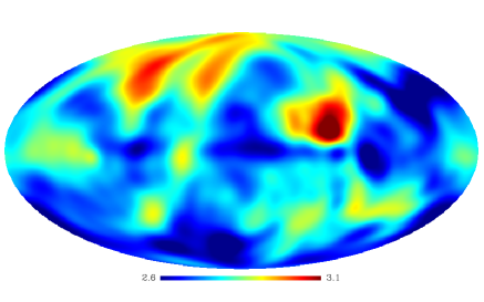
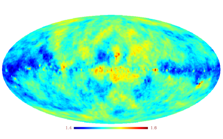
Figure 1: Spectral index maps of synchrotron (top) and dust (bottom) components, used in the simulated sky

Our simulation of the diffuse emission exploits all the available information from existing public pre-Planck surveys. The simulated CMB map is based on a standard $\Lambda$CDM model consistent with WMAP 5-years cosmological parameters, with a tensor to scalar ratio $r=0.1$. The rms fluctuations of the CMB are expressed in antenna temperature, $T_{\rm A,CMB}(\nu)$, whose frequency dependence writes:

$$T_{\rm A,CMB}(\nu)\propto\frac{(h\nu/kT_{\rm CMB})^{2}\exp(h\nu/kT_{\rm CMB})}{(\exp(h\nu/kT_{\rm CMB})-1)^{2}}\ ,$$ (34)

where $h$ is the Planck constant, $k$ the Boltzmann constant, $T_{\rm CMB}=2.726\,$K.

The simulation of the diffuse Galactic emissions is based on Miville-Deschênes & Boulanger (2007) and implemented by the Planck working group on Component Separation. The starting point towards building the synchrotron emission template is an extrapolation of the 408 MHz map of Haslam et al. (1982) from which an estimate of the free-free emission has been removed. Due to the poor resolution of the Haslam map (52 nominal arcmin) small structures have been artificially added using the procedure presented in Miville-Deschênes & Boulanger (2007). The fraction of polarization is derived from a model of the magnetic field including spiral and turbulent components based on WMAP 5yr results. On large scales ($>5\,$deg) the polarisation angle is WMAP constrained; on smaller scales it relies on the Galactic magnetic field model. The spectrum, in antenna temperature, is assumed to follow a power law:

$$T_{\rm A,synch}(\nu)\propto\nu^{-\beta_{s}}\ ,$$ (35)

where the synchrotron spectral index $\beta_{s}$ varies with the position on the sky. To this aim, we use the map of spectral indices given by Giardino et al. (2002). This map shows structures on scales of up to 10 degrees, with $\beta_{s}$ varying from 2.5 to 3.2 (see the top panel of Fig. 1).

The simulation of the polarized thermal dust emission is based on model 3 of Finkbeiner et al. (1999). This model extrapolates the $100\,\mu$m brightness map (Schlegel et al., 1998) assuming grey body spectra:

$$T_{\rm A,dust}(\nu)\propto\frac{\nu^{\beta_{d}+1}}{\exp(h\nu/kT_{\rm dust})-1},$$ (36)

with $T_{\rm dust}=18\,$K and spatially varying emissivity index $\beta_{d}$, obtained from the map of $100/240\,\mu$m flux density ratios published by Schlegel et al. (1998). The map of $\beta_{d}$ shows structure down to arcminute scales (see the bottom panel of Fig. 1) with $\beta_{d}$ varying from 1.44 to 1.6. The polarized intensity is obtained multiplying the brightness map by a polarization fraction map extracted from WMAP 5yr data with the help of the model of the previously mentioned Galactic magnetic field model. In this simulation the polarization fraction is not frequency dependent.

Component maps have been produced at central frequencies of all Planck channels. They are then co-added and smoothed with nominal Gaussian beams (see Table 1). A white inhomogeneous noise is synthesized using the block diagonal part of the predicted noise covariance matrix given the Planck nominal integration time (14 months) and scanning strategy. The correlation between noise in different Stokes parameters for each pixel has also been reproduced. This dataset has been complemented with the simulated WMAP 23 GHz map after 5 years of survey. This map has a resolution of 58 arcmin and the noise is simulated starting from the diagonal noise covariance provided by the WMAP team (http://lambda.gsfc.nasa.gov). This ancillary product is used to help tracing the low frequency foreground component for the CCA run, as described in § 5.

Table 1: Central frequencies, $\nu$, and angular resolutions for the Planck channels considered in the present study

$\nu\,$(GHz)	30	44	70	100	143	217	353
FWHM (arcmin)	33	24	14	9.5	7.1	5.0	5.0

5 Estimating the mixing matrix parameters and errors with CCA

We applied both pixel and harmonic domain CCA to the polarized Planck simulations described in the previous section (7 frequencies from 30 GHz to 353 GHz), with and without the ancillary 23 GHz WMAP channel. For the harmonic domain version we use the channel maps at their native resolution. In the application to polarized data we perform separated runs of the Q and U maps so the $\mathbf{c}(\hat{\ell})$ in eq. (18) simply represent cross-power spectra. We can evaluate the local mixing matrix using both information from Q and U maps. In practice, due to the lower foregrounds signal in the U maps,the mixing matrix is basically defined by the Q maps analysis only. The application of pixel-domain CCA requires that all the channel maps have the same resolution. Thus we preliminarily degraded the maps to the resolution of the lowest frequency channel (33 arcmin to work with Planck data only, 58 arcmin to include WMAP 23 GHz channel) convolving the maps with a Gaussian beam. The data model includes three diffuse components: CMB, synchrotron and thermal dust, parameterized as in eqs. (34), (35) and (36) respectively. We estimated two free parameters, the synchrotron and the dust indices, which were allowed to vary in the ranges $2.3\leq\beta_{s}\leq 3.5$ and $1.\leq\beta_{d}\leq 2.5$, while we kept $T_{\rm dust}=18\,$K. We note that we do not explicitly account for any modeling error in our analysis, as the mixing matrix parametrization assumed by CCA exactly reflects the one exploited for the data generation. Thus, the only systematic error is given by the assumption that the spectral properties are constant within sky patches. Including the effect of an imperfect modeling is beyond the scope of this paper, whose goal is to evaluate CCA performances per se. The problem was addressed in Bonaldi et al. (2007) where several models for the anomalous emission were tested for the analysis of WMAP temperature data with CCA. In any case, we believe that such model uncertainties should be less severe in polarization.

The choice of the patch size for the CCA run is a trade-off between the need to have uniform foreground properties, which calls for small patches, and the need to have enough statistics, which calls for bigger ones. The latter is obviously related to the instrumental resolution of the data, as the statistics is ultimately determined by the number of resolution elements in the considered region of the sky. In the case of harmonic-domain CCA we have the additional constraint of the maximum patch size allowed by the planar approximation. However, the possibility of this version of CCA to handle frequency-dependent instrumental beams, and thus to exploit the full resolution, generally allows the use of smaller patches compared to pixel domain CCA. In this work we divide the sky in square patches for both pixel domain and harmonic domain CCA. The pixel based version does not suffer of any constraint regarding the shape of the patch. The current harmonic version instead can work only on square regions. We adopt a patch size of $40^{\circ}\times 40^{\circ}$ for pixel-domain CCA, of $30^{\circ}\times 30^{\circ}$ for harmonic-domain CCA. The centers of the patches are equally spaced in latitude and longitude with shifts of $3^{\circ}$, up to a maximum central latitude of $\pm 30^{\circ}$ so that we have 2520 patches in the sky. This helps us to build a smooth spectral index map and allows a more localized spectral index estimation, as described in § 6. Moreover this provides the redundancy needed for error estimation as described in § 3.3.2, for which we considered samples of patches overlapping by more than 60%. We note however that this purely geometrical partition of the sky is not driven by any astrophysical reason. If we could achieve a partition that maximizes the uniformity of the spectral properties within each patch, the CCA estimation would be more accurate. The full run took $\sim$ 10 hours on a parallel machine at NERSC using 120 processors. Convergence has been reached in $\sim 80\%$ of the patches for pixel domain CCA and $\sim 90\%$ of the patches for harmonic domain CCA.

5.1 Evaluation of the results

5.1.1 Actual errors on parameter estimation

Ideally, to evaluate the quality of CCA results we should compare the true synchrotron and dust spectral indices with the estimated ones for each position in the sky. However, CCA only provides spectral indices per patch, and the true spectral indices in general vary within the patch. Thus we computed:

$$\Delta\mathbf{p}=\mathbf{\bar{p}}-\mathbf{\hat{p}},$$ (37)

where $\mathbf{\bar{p}}=[\bar{\beta}_{s},\bar{\beta}_{d}]$ are the flux weighted averages of the true parameters over the patch and $\mathbf{\hat{p}}=[\hat{\beta}_{s},\hat{\beta}_{d}]$ are the estimates provided by CCA. This choice for the “true” spectral indices per patch seems to be the most appropriate because the CCA results mostly reflect the spectral properties of the brightest foreground structures in the considered patch. Such bright structures are obviously those that need to be more accurately removed to produce a clean CMB map. In any case, a systematic difference is expected because the “true” mean spectral indices and the ones recovered by CCA have somewhat different meanings.

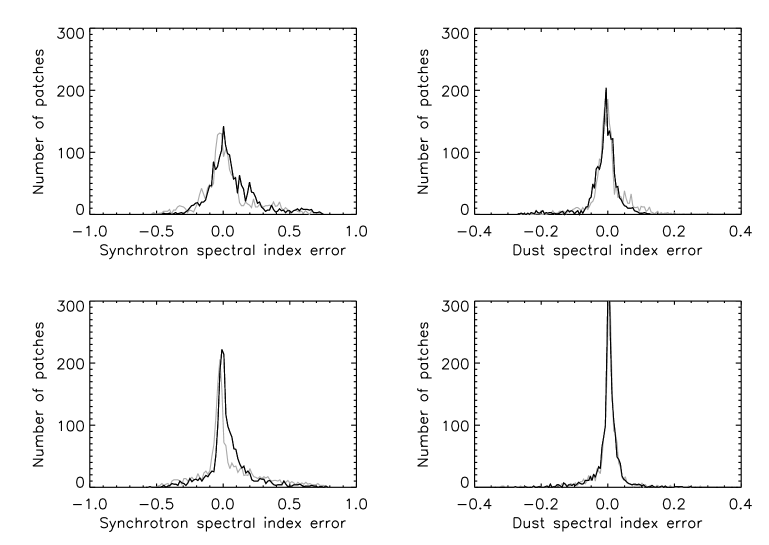
Figure 2: Distribution of errors in the recovery of synchrotron (left) and dust (right) spectral indices for the full sample of sky patches using only the simulated Planck maps (grey) and adding the simulated WMAP 23 GHz map (black). Top: pixel domain CCA; bottom: harmonic domain CCA

In Fig. 2 we show for each parameter and for both pixel domain and harmonic domain CCA the distribution of “true” errors for the full sample of patches obtained from simulated Planck Q maps with and without the simulated WMAP 23 GHz channel. Table 2 reports the offset (from zero) of the mean and the standard deviation of a gaussian fit computed for each histogram. We note that the offset is in some cases comparable with the rms; this systematic error is induced by the spatial variability of the true indices, as mentioned above. We verified that, once we adopt spatially-uniform spectral indices for the data generation ($\beta_{s}=2.9$ and $\beta_{d}=1.7$), the offset disappears while the width of the distributions is almost unchanged. Errors in the recovery of the synchrotron spectral index are bigger than those for the dust. This is due to the fact that the dust component is much better traced by the frequency coverage of Planck. The inclusion of the WMAP 23 GHz channel almost cancels the offset from zero of the mean error on the synchrotron spectral index for harmonic domain CCA, while slightly increasing the rms value (see Table 2). For pixel domain CCA the advantage of a broader frequency range yielded by the inclusion of the 23 GHz map is more than compensated by the degradation of the resolution of the whole data set; as a result, both the mean offset and the rms value of errors somewhat increase. In the following we only consider the results obtained with Planck maps alone for pixel domain CCA, and with Planck $+$ 23 GHz data for harmonic domain CCA. The rms errors in the synchrotron and dust spectral indices are $0.08$ and $0.019$ respectively for pixel domain CCA, $0.045$ and $0.009$ respectively for harmonic domain CCA. Thus the harmonic domain CCA performs better than the pixel domain version.

Table 2: Offsets of the mean and rms values for the error distributions in Fig. 2 (Planck dataset/Planck + 23 GHz data set)

		offset	rms
Synchr.	Pixel CCA	-0.009/0.016	0.080/0.107
	Harmonic CCA	-0.027/0.002	0.036/0.045
Dust	Pixel CCA	-0.005/-0.004	0.019/0.022
	Harmonic CCA	0.005/0.003	0.010/0.009

Figure 3: Absolute values of estimated vs actual error on synchrotron (left) and dust spectral index (right) for the harmonic domain CCA; error estimation through the marginal distribution method. Dots are the values for individual patches, squares and error bars are the median values and quartiles computed for groups of 100 points, respectively

.

5.1.2 Actual versus estimated errors

As illustrated by Fig. 3 the errors estimated via the marginal distribution method (§ 3.3.1.) are well correlated to the “true” errors above $\Delta\beta_{s}\simeq 0.05$ or $\Delta\beta_{d}\simeq 0.01$. When the estimated errors are small, the “true” errors are small as well, although the two quantities are not correlated. This is due to the effect of noise which hampers the calculation of the marginal probability distribution with sufficient accuracy. The largest errors are moderately underestimated; this is not particularly worrisome however, since large errors correspond to regions where the foreground signals are very weak and can be removed with sufficient accuracy adopting the mean parameter values determined in the rest of the sky. The spatial redundancy error estimation method (§ 3.3.2) applied to both pixel and harmonic CCA yields estimated errors systematically lower than the “true” ones. However, the latter are well matched by the third quartiles of the distribution of estimated errors. As expected, the spatial redundancy method performs better for the harmonic than for the pixel domain CCA, thanks to the higher spatial resolution ($30^{\circ}\times 30^{\circ}$ versus $40^{\circ}\times 40^{\circ}$ patches).

Despite the non-idealities mentioned above, errors estimates produced by both methods are good enough to be exploited in the next step of our pipeline. In the following analysis we will restrict ourselves to values of each spectral index $\beta$ within the range $|\hat{\Delta}\beta|<\mu_{\hat{\Delta}\beta}+\sigma_{\hat{\Delta}\beta}$, where $\hat{\Delta}\beta$ is the estimated error on $\beta$ and $\mu_{\hat{\Delta}\beta}$ and $\sigma_{\hat{\Delta}\beta}$ are the mean and the standard deviation of the estimated errors over all the patches. This set of values constitutes the final sample. Figure 4 compares the rms values of the actual estimation errors as a function of Galactic latitude for both the full and the final sample, showing that indeed this procedure removes the most discrepant values. As already pointed out by Bonaldi et al. (2007), the performance of CCA is highly dependent on the intensity of the foreground signal in the considered patch. Estimations of the spectral parameters are better close to the Galactic plane and worsen with increasing Galactic latitude where, however, the foreground signals are anyway very weak and their removal is therefore not a critical issue. Our method allows us to flag the worse estimates and to replace them with average values determined in the rest of the sky.

Figure 4: Rms errors in the estimation of spectral indices as a function of Galactic latitude. Solid lines: full sample; dashed lines: final sample obtained with spatial redundancy error estimation method; dotted lines: final sample obtained with marginal distribution error estimation method. The errors increase at high Galactic latitudes, where the foreground signal are weak and there removal is therefore not a critical issue.

6 Building full-sky maps of spatially-varying spectral indices

Figure 5: Dependence of the weight w1 on the distance from the patch center normalized to half of the patch size $\Delta$

The information on spectral parameters provided by CCA for sky patches can be combined to build full-sky maps of the estimated, spatially-varying spectral indices, and the associated estimation error maps. We use the Healpix (Górski et al., 2005) pixelization, with resolution parameter NSIDE=64, corresponding to pixel areas of about 1 square degree. Let us consider the component $\rm p$ (e.g. the synchrotron spectral index) of the parameter vector $\mathbf{p}$. Due to the partial overlap of sky patches, the $j$-th pixel of the Healpix map, whose position on the sky is centered at $\mathbf{r_{j}}$, belongs to several different patches for each of which we have obtained an estimate of $\rm p$. We can therefore compute a weighted mean of the values of the parameter $\rm p_{\mathbf{j}}$ and of the error $\Delta\rm p_{\mathbf{j}}$ as follows:

$$\rm p_{j} = \frac{\sum_{i=1}^{N}{\rm p}(\mathbf{r}_{i})\cdot w1(\mathbf{r}_{i},\mathbf{r}_{j})\cdot w2(\mathbf{r}_{i})}{\sum_{i=1}^{N}w1(\mathbf{r}_{i},\mathbf{r}_{j})\cdot w2(\mathbf{r}_{i})},$$ (38)

$$\Delta\rm p_{j} = \frac{\sum_{i=1}^{N}\Delta{\rm p}(\mathbf{r}_{i})\cdot w1(\mathbf{r}_{i},\mathbf{r}_{j})}{\sum_{i=1}^{N}w1(\mathbf{r}_{i},\mathbf{r}_{j})},$$ (39)

where the sum is over all patches in the final sample, defined in § 5.1.2, and $w1$ and $w2$ are weight functions. The former, $w1(\mathbf{r}_{i},\mathbf{r}_{j})$, depends on the distance between the $j$-th pixel and the center of the $i$-th patch, $||\mathbf{r}_{i}-\mathbf{r}_{j}||$, normalized to the half size of the patch, $\Delta/2$. We used the function shown in Fig. 5, equal to 1 for $||\mathbf{r}_{i}-\mathbf{r}_{j}||\ll\Delta/2$, and equal to 0 for $||\mathbf{r}_{i}-\mathbf{r}_{j}||\,\lower 2.0pt\hbox{${>\atop\hbox{\raise 4.0pt\hbox{$\sim$}}}$}\,\Delta/2$. The weight $w2(\mathbf{r}_{i})=w2(\Delta\rm p(\mathbf{r}_{i}))$ depends on the estimated error for the $i$-th patch trough the relation:

$$w2(\mathbf{r}_{i})=1-\frac{\Delta\rm p(\mathbf{r}_{i})}{\rm max(\Delta\rm p(\mathbf{r}_{i}))},$$ (40)

approaching 1 as $\Delta\rm p(\mathbf{r}_{i})\rightarrow 0$ and approaching 0 when $\Delta{\rm p}(\mathbf{r}_{i})\rightarrow{\rm max}(\Delta\rm p(\mathbf{r}_{i}))$, ${\rm max}(\Delta\rm p(\mathbf{r}_{i}))$ being the maximum error estimated for the final sample.

We can associate to the $j$-th pixel of the Healpix map, whose position on the sky is $\mathbf{r_{j}}$, the parameter $\rm p_{\mathbf{j}}$ and the error $\Delta\rm p_{\mathbf{j}}$ as follows:

Our spectral index and error maps are undefined in regions, mostly at high Galactic latitudes ($|b|>30^{\circ}$), where the Galactic emissions are too low and the CCA cannot produce reliable estimates of their spectral parameters. For these regions we have adopted the mean values of the parameters found for the rest of the sky, using a smoothing function to soften edge effects.

Figure 6: Distribution of residual (true-estimated) synchrotron (left) and dust (right) spectral index maps in the latitude range $-30^{\circ}<b<30^{\circ}$. The pixel size used is $\sim 0.84$ square degree (nside 64). Top: pixel domain CCA; bottom: harmonic domain CCA.

6.1 Evaluation of the quality of the results

To evaluate the quality of the maps of estimated spectral parameters, we looked at the residual spectral index maps. To compute those maps, we regridded the true input spectral index maps to NSIDE=64, the resolution of the estimated maps. In Fig. 6 we show the distributions of residuals (true minus estimated spectral indices) with a Gaussian fit superimposed. The histograms only contain the pixels in the latitude range $-30^{\circ}<b<30^{\circ}$ where the spectral indices have been estimated. Overall, the results are encouraging. Again the harmonic domain CCA works better than the pixel domain version for both dust and synchrotron spectral parameters. Both approaches give negligibly small mean offsets from the true values, but the harmonic CCA has smaller dispersions of the residuals ($\sigma_{s}\simeq 0.08$, $\sigma_{d}\simeq 0.01$) than the pixel domain CCA ($\sigma_{s}\simeq 0.11$, $\sigma_{d}\simeq 0.02$).

7 Reconstruction of the components with GLS

Having shown that the harmonic domain CCA is superior to the pixel domain version, we have used its estimates of synchrotron and dust spectral indices to build the spatially-varying mixing matrix $\mathbf{H}$ and the reconstruction matrix $\mathbf{W}$ given by eq. (32). To recover each emission component we have applied the reconstruction matrix [see eq. (11)] to the simulated data for Planck channels in the frequency range from 70 to 217 GHz, where the CMB is the least contaminated by foreground emissions. On the other hand, just for the same reason, this frequency range is not optimal for the recovery of foreground emissions. All the maps were smoothed to the resolution of the 70 GHz channel (14 arcmin FWHM). We also performed a run at a 60 arcmin resolution to reduce the contribution of instrumental noise, so that we can better appreciate the effect of component separation errors on the reconstructed maps. Besides the component maps [eq. (11)], we also computed the variance due to instrumental noise [eq. (33)] and to residual foreground contamination. The latter is estimated by propagating the errors on the mixing matrix parameters to the separated components as descibed in §  3.5. In particular we assume that the spatial correlation of separation errors in the spectral index in each pixel are the same as those in the spectral index map itself. Thus, in order to evaluate and propagate the error in the outputs, we construct Monte Carlo variations of the estimated spectral index maps. In doing this, we further simplify our treatment by only taking into account the two-point correlation function of the map.

Therefore, if $\beta_{s}$ and $\beta_{d}$ are the maps of the estimated synchrotron and dust spectral indices respectively, and $err\beta_{s}$, $err\beta_{d}$ the corresponding estimated error maps, for the i-th run we obtain the perturbed spectral index maps $\beta_{s}^{i}$ and $\beta_{d}^{i}$ as follows:

$${\rm\beta_{s}^{i}} = {\rm\beta_{s}}+\Delta_{s}\cdot{\rm err\beta_{s}}$$ (41)

$${\rm\beta_{d}^{i}} = {\rm\beta_{d}}+\Delta_{d}\cdot{\rm err\beta_{d}},$$

where $\Delta_{s}$ and $\Delta_{d}$ are two maps with zero mean and unit rms synthesized from the 2-point correlation function extracted from the corresponding estimated spectral index map.

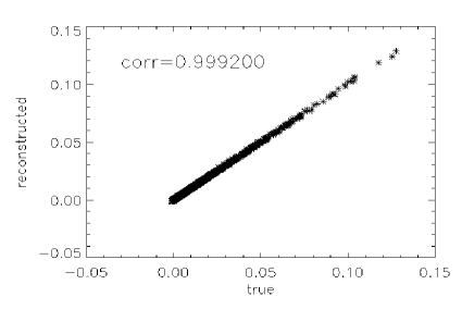
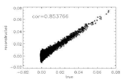
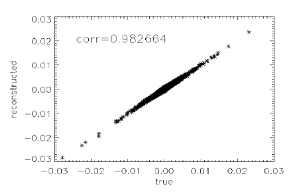
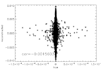
Figure 7: Correlations between the true and the reconstructed $Q$ and $U$ maps of Galactic components for $\simeq 1^{\circ}$ pixels. Upper left panel: dust $Q$ (correlation coefficient $\simeq 0.99$); upper right panel: synchrotron $Q$ (correlation coefficient $\simeq 0.85$); lower left panel: dust $U$ (correlation coefficient $\simeq 0.98$ ). The synchrotron $U$ (lower right panel) was not detectable.

For each set of fake spectral index maps obtained through eqs. (41) we performed the source reconstruction by GLS, thus obtaining as many sets of output components. We computed the variance due to separation for a certain component as the variance of all the results for that component.

Figure 8: True rms fluctuations of input polarized components at the reference frequency of 70 GHz as a function of Galactic latitude for a $60^{\prime}$ resolution (solid line) compared with estimated error due to instrumental noise (dashed line) and estimated error due to residual contamination for the marginal distribution (dotted line) and spatial redundancy (dashed-dotted line) error estimation methods. Upper panels: Q Stokes parameter; lower panels: U Stokes parameter.

In Fig. 8 we show for all the components reconstructed with $60^{\prime}$ resolution the rms of the true input component as a function of Galactic latitude, compared to the $\sigma$ due to noise and imperfect separation, computed from the variances output by our method. Even at this low resolution instrumental noise dominates except close to the Galactic plane where the S/N ratio is $\sim 10$. The error estimation yielded by the marginal distribution method is more conservative than the one obtained with spatial redundancy method; the two estimates typically differ by 30%.

Figure 9: Cross spectra [eq. (42)] between the true and the reconstructed component for dust (left) and synchrotron emission (right).

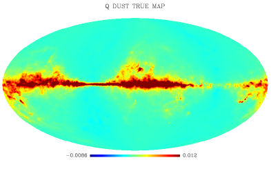
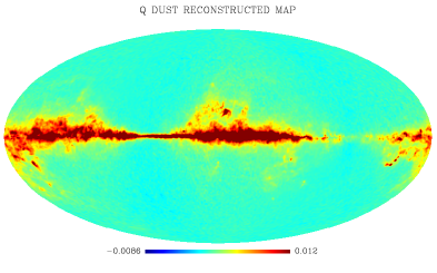
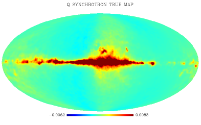
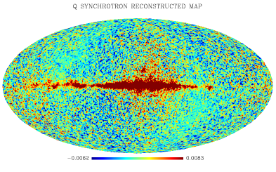
Figure 10: True and reconstructed maps for dust (top) and synchrotron emission (bottom).

Figure 11: Comparison of true (diamonds) and estimated rms errors as a function of Galactic latitude at 70 GHz for $Q$ (upper panels) and $U$ (lower panels) maps. Dotted lines: marginal distribution method (§ 3.3.1); dot-dashed lines: spatial redundancy method (§ 3.3.2).

Figure 12: Noiseless case: comparison of true (diamonds) and estimated rms errors as a function of Galactic latitude at 70 GHz for $Q$ (upper panels) and $U$ (lower panels) maps. Dotted lines: marginal distribution method (§ 3.3.1); three dots-dashed lines: spatial redundancy method (§ 3.3.2). At high Galactic latitudes, where both our methods overestimate the component separation errors, such errors are irrelevant compared to uncertainties due to instrumental noise.

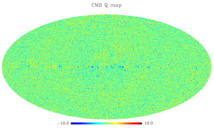
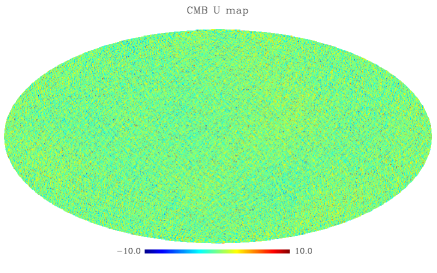
Figure 13: Full-sky $Q$ (left) and $U$ (right) CMB maps obtained by CCA for the noiseless case.

7.1 Quality of the reconstructed component maps

In Fig. 7 we compare the recovered $Q$ and $U$ maps of synchrotron and dust emission with NSIDE=64 (resolution $\simeq 1^{\circ}$). The agreement is almost perfect for dust (correlation coefficient of 0.98–0.99), and very good for the synchrotron $Q$ (correlation coefficient of 0.85). The synchrotron $U$ map could not be reconstructed because of the very low S/N ratio (see Fig. 8) due to the choice of frequency channels, that left out the low frequency ones (30 and 44 GHz, and WMAP 23 GHz) where the synchrotron is much stronger.

As another figure of merit, we computed the normalized correlation multipole by multipole between the true and reconstructed map:

$$\frac{\langle C_{\ell}^{\rm cross}\rangle^{2}}{\langle C_{\ell}^{\rm true}\rangle\langle C_{\ell}^{\rm stim}\rangle},$$ (42)

where $C_{\ell}^{\rm true}$ and $C_{\ell}^{\rm stim}$ are the auto-spectra of the true and the reconstructed component, and $C_{\ell}^{\rm cross}$ the cross-spectrum between the two. Figure 9 shows that, for dust, the cross-correlation is close to unity on all the relevant scales. The same is true for synchrotron, on scales larger than a few degrees; on smaller scales the correlation drops because the instrumental noise dominates. In Fig. 10 we show the comparison between the true and the reconstructed Q synchrotron and dust emission maps.

7.2 Assessment of the component separation error estimations

As outlined above, our method outputs two rms error maps, one for instrumental noise and the other for component separation errors. The actual error map for each component is simply computed as the residual map, i.e. the difference between the reconstructed map of a component and the true one at the same resolution. This residual map contains both noise and component separation errors, and thus has to be compared to the global estimated error map, obtained summing the variances of the two estimated contributions.

In Fig. 11 we show the standard deviations of the residuals as function of Galactic latitude (diamonds) compared to the total error yielded by both our error estimation methods for the 60 arcmin resolution (lines). The results are generally very good, as the total error is correctly predicted. On the other hand, since we are generally noise dominated, this figure cannot tell much about the goodness of our component separation error estimates, except for dust close to the Galactic plane, where the error estimate turns out to be very successful. We note however that, as we are using a linear estimator [eq. (11)] to reconstruct the components, our final results can be decomposed into a noiseless term, only affected by component separation errors, plus a noise term:

$$\mathbf{\hat{s}}=\mathbf{Wy}=\mathbf{W[Hs]}+\mathbf{Wn}.$$ (43)

Here $\mathbf{Hs}$ is a noiseless dataset, obtained exactly as described in § 4 but without adding noise. By combining the noiseless dataset with the same reconstruction matrix estimated in the noisy case, we obtain a set of reconstructed components having the same component separation errors as before, but without noise. This allows us to test the quality of component separation error estimates. The results, shown in Fig. 12, are very encouraging. Even if component separation errors are in general highly subdominant, the marginal distribution error estimation method is able to correctly estimate them at low and intermediate Galactic latitudes (at high Galactic latitudes the component separation errors are overestimated but are anyway irrelevant compared to errors due to noise). On the other hand the spatial redundancy error estimation method is occasionally underestimating the true errors at low latitude. In Fig. 13 we show, as an example, the CMB $Q$ and $U$ reconstructed maps in the noiseless case. A visual inspection does not reveal the presence of residual Galactic contamination except for a tiny strip on the Galactic plane.

8 CMB power spectrum estimation

To assess the quality of the Stokes $Q$ and $U$ CMB maps obtained with the CCA component separation we compare their estimated angular power spectra (APS) to the input model used to generate the simulation. In doing so we propagate to the power spectra the component separation errors described above. We employ the ROMAster code, a pseudo-$C_{\ell}$ estimator based on MASTER approach  (Hivon et al., 2002) and extended to cross-power spectra (Polenta et al., 2005) and polarization (see e.g. Kogut et al., 2003, for a similar formalism). It is well known that the pseudo $C_{\ell}$ approach to the CMB power spectrum estimation is sub-optimal for the lowest multipoles where other techniques are more appropriate (see, e.g., Gruppuso et al., 2009). However, a pseudo-$C_{\ell}$ estimator is enough for our purpose of assessing the quality of the reconstructed CMB polarization maps in the presence of noise and component separation errors.

We exclude from the analysis the regions that are most contaminated by residual foreground contributions as estimated in the previous section. For this purpose we build a mask based on our reconstruction errors, flagging all pixels where the sum of the variance errors on the CMB $Q$ and $U$ maps is greater than the mean value of the same quantity across the whole map. The resulting mask is shown in Fig. 14 and excludes less than 10% of the sky.

Having only one final map per astrophysical component, we do not rely here on a cross spectrum analysis but on an auto-spectrum approach. This is rather general, and achieves a lower final noise variance than the cross spectrum approach (see, e.g., Polenta et al., 2005). The drawback is that we need to model and subtract a noise bias in the data. To this extent, we computed the noise bias on the CMB EE power spectrum by means of 1000 simulated noise maps. To obtain each of them, we simulated one noise map for each channel included in the reconstruction of the CMB (70, 100, 143 and 217 GHz), equalized the resolution of all channels to $14^{\prime}$, and combined them with the reconstruction matrix $\mathbf{W}$ as described in the previous section. ROMAster uses these Monte Carlo data to subtract the noise bias, as well as to estimate errors on the APS due to noise by computing the empirical variance of the realization.

To compute the error bars due to residual foreground contamination, we produced a further set of 100 CMB maps by perturbing the input spectral index maps as described in the previous section. For each of them we repeated the computation of the power spectrum and corrected for the noise bias, relying for the latter purpose on a smaller ($\sim 10$) set of noise-only maps. The noise bias has been estimated each time with the reconstruction matrix used to obtain the corresponding CMB map. Even if quite computationally demanding, this procedure is needed because we are in the noise-dominated regime, and a small error in the noise bias can substantially affect the estimation of the polarized power spectrum. Once we got our 100 unbiased CMB power spectra, we finally computed the errors due to component separation as the standard deviation of the sample for each considered multipole bin.

In Fig. 15 we show the noise and the component separation error bars compared to the EE power spectrum of the fiducial model. As we can see, the noise contribution is dominating even on the smallest multipoles over the component separation error, which is at most a small correction to the error budget. In Fig. 16 we show the EE power spectrum estimated in a realistic Planck case (diamonds); the 1$\sigma$ errors are shown by the shaded area. The results for the noiseless case (squares with the component separation error bars) show that the accuracy of our estimation of the power spectrum is not limited by component separation but rather by the effect of the noise. The overall quality of the recovered spectrum is impressive, especially when compared to the total Galactic emission at 70 GHz, shown on top of the plot.

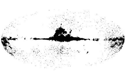
Figure 14: Mask used for the computation of the EE power spectrum, excluding 9% of the sky on the basis of the estimated variance due to component separation on the CMB Q and U maps.

Figure 15: EE power spectrum of the input model (solid) compared to the rms errors due to noise (dot-dashed line), separation (dashed line) and total (solid line). The dotted line represents the associated cosmic variance error.

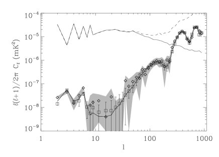
Figure 16: Recovered EE power spectrum in the realistic Planck case (diamond) and 1 $\sigma$ uncertainties (shaded area); recovered EE power spectrum in the noiseless case (squares) with 1 $\sigma$ component separation error bars; EE input CMB map (gray solid line). On top of the plot we also show, for comparison, the total Galactic emission of our simulation at 70 GHz (solid line); the dashed line includes the effect of the 70 GHz Planck noise.

Although a discussion on the detectability of CMB B-modes is beyond the scope of this paper (see Betoule et al., 2009; Efstathiou & Gratton, 2009, for recent analyses), we briefly address here the potential of the CCA in this respect. An interesting point, raised by Efstathiou et al. (2009), is that some foreground subtraction methods, such as the ILC, are not well-suited for applications to B-mode detection, as they introduce an offset caused by the dominant E-mode polarization pattern which prevents estimating B modes even in absence of noise. To check whether this also applies to our component separation pipeline, we estimated the CMB B-mode power spectrum from the CMB maps recovered by the CCA in the noiseless case. It is important to note, however, that this cannot be really considered as the application of our pipeline to an ideal (noiseless) experiment because, while the component reconstruction has been made by setting to zero the noise term in eq. (43), the spectral parameters going into the reconstruction matrix used to perform component separation are those estimated by assuming the real pre-flight estimates of Planck noise level for the nominal mission duration (14 months). The errors on foreground spectral parameters, and therefore those on the recovered CMB map, are thus substantially larger than those expected for an ideal noiseless experiment.

The results are shown in Fig. 17. For the tensor to scalar ratio adopted in the simulations ($r=0.1$), our component separation method proves to be capable of recovering the B-mode power spectrum over a quite broad multipole range without any noticeable spurious feature due to residual foreground contamination or to cross-correlation with the E-mode. Note that the error bars due to component separation shown in Fig. 17 are estimated in the presence of noise while the CMB recovery is made using noiseless maps. Since the noise dominance will be much stronger for the B-mode than for the E-mode, the subtraction of the noise bias will be a very delicate and computationally demanding, but conceptually easy, operation.

Figure 17: Recovered B-mode power spectrum in the noiseless case (squares with 1$\sigma$ component separation error bars) compared with the input model (solid line).

9 Conclusions

We presented and tested on realistically simulated Planck polarization data a pipeline for component separation based on the CCA method (Bedini et al., 2005; Bonaldi et al., 2006, 2007). This method exploits the data statistics to estimate the frequency behaviour of the diffuse components superimposed to the CMB, described in terms of a limited set of parameters, which in our case are synchrotron and thermal dust spectral indices.

The most recent harmonic domain version of CCA proved to be even superior to the original pixel domain one, which however gave very good results for simulated Planck (Bonaldi et al., 2006; Leach et al., 2008) and WMAP data (Bonaldi et al., 2007) temperature data. As another improvement, we worked out a method to combine the results obtained with CCA on several regions of the sky to provide spatially-varying maps of spectral indices, with rms errors of only 0.015 for the dust component and of 0.08 for the synchrotron component, exploiting polarization data only (Planck plus the WMAP 23 GHz channels).

Perhaps the most important new result of this paper is the elaboration, for the first time, of successful methods for estimating component separation errors. We presented two alternative error estimation methods for the CCA, relying on completely different assumptions (one is based on studying the marginal probability for each parameter estimated, the other on the redundancy of results for different patches of the sky) so that they can also be used to cross-check the results. A first application of these methods allowed us to identify the most uncertain values of the parameters and to compute the appropriate weights to be used to combine the estimates in different regions of the sky to build a smooth map of foreground spectral indices.

The components were reconstructed with a Generalized Least Square (GLS) solution in pixel space, which allowed us to fully exploit the spatially-varying information obtained. Even if the choice of the channels used in the reconstruction is optimized for the CMB, we were able to reconstruct a very accurate dust polarization map (correlation coefficient $\sim 1$ with the input maps). Errors in the estimation of the foreground spectral indices were successfully propagated to the foreground maps. They turned out to be well below those due to instrumental noise, except for the dust component close to the Galactic plane.

As for the CMB, we used ROMAster to estimate the polarization E-mode power spectrum from the reconstructed CMB map and found negligible effects by the residual foreground contamination even masking only 10% of the sky. Again the component separation errors, propagated to the power spectrum, were found to be subdominant with respect to noise. We also showed that our component separation method can be useful to tackle B-mode detection, once the experimental noise level allows it.

References

- Bedini et al. (2005) Bedini L., Herranz D., Salerno E., Baccigalupi C., Kuruouglu E. E., Tonazzini A., 2005, EURASIP Journal on Applied Signal Processing, Vol. 2005 (Applications of Signal Processing in Astrophysics and Cosmology), Guest Editors Kuruoglu E. E. and Baccigalupi, C., p. 2400-2412, 2005, 2400
- Bedini & Salerno (2007) Bedini L., Salerno E., 2007, in Bruno Apolloni R. J. H., Jain L., eds, Knowledge-Based Intelligent Information and Engineering Systems Extracting astrophysical sources from channel-dependent convolutional mixtures by correlated component analysis in the frequency domain. Springer, pp 9 – 16
- Bedini & Salerno (2008) Bedini L., Salerno E., 2008, Fourier-domain implementation of correlated component analysis, with error estimation Internal Report B4-007, CNR-ISTI, Pisa
- Bennett et al. (2003) Bennett C. L., Hill R. S., Hinshaw G., Nolta M. R., Odegard N., Page L., Spergel D. N., Weiland J. L., Wright E. L., Halpern M., Jarosik N., Kogut A., Limon M., Meyer S. S., Tucker G. S., Wollack E., 2003, VizieR Online Data Catalog, 214, 80097
- Betoule et al. (2009) Betoule M., Pierpaoli E., Delabrouille J., Le Jeune M., Cardoso J., 2009, A&A, 503, 691
- Bonaldi et al. (2006) Bonaldi A., Bedini L., Salerno E., Baccigalupi C., de Zotti G., 2006, MNRAS, 373, 271
- Bonaldi et al. (2007) Bonaldi A., Ricciardi S., Leach S., Stivoli F., Baccigalupi C., de Zotti G., 2007, MNRAS, 382, 1791
- Brandt et al. (1994) Brandt W. N., Lawrence C. R., Readhead A. C. S., Pakianathan J. N., Fiola T. M., 1994, ApJ, 424, 1
- de Bernardis et al. (1999) de Bernardis P., Ade P. A. R., Artusa R., Bock J. J., Boscaleri A., Crill B. P., De Troia G., et al., 1999, New Astronomy Review, 43, 289
- de Bernardis et al. (2009) de Bernardis P., Bucher M., Burigana C., Piccirillo L., 2009, Experimental Astronomy, 23, 5
- Delabrouille & Cardoso (2009) Delabrouille J., Cardoso J., 2009, in V. J. Martinez, E. Saar, E. M. Gonzales, & M. J. Pons-Borderia ed., Lecture Notes in Physics, Berlin Springer Verlag Vol. 665 of Lecture Notes in Physics, Berlin Springer Verlag, Diffuse Source Separation in CMB Observations. pp 159–+
- Efstathiou & Gratton (2009) Efstathiou G., Gratton S., 2009, Journal of Cosmology and Astro-Particle Physics, 6, 11
- Efstathiou et al. (2009) Efstathiou G., Gratton S., Paci F., 2009, MNRAS, 397, 1355
- Eriksen et al. (2006) Eriksen H. K., Dickinson C., Lawrence C. R., Baccigalupi C., Banday A. J., Górski K. M., Hansen F. K., Lilje P. B., Pierpaoli E., Seiffert M. D., Smith K. M., Vanderlinde K., 2006, ApJ, 641, 665
- Finkbeiner et al. (1999) Finkbeiner D. P., Davis M., Schlegel D. J., 1999, ApJ, 524, 867
- Giardino et al. (2002) Giardino G., Banday A. J., Górski K. M., Bennett K., Jonas J. L., Tauber J., 2002, A&A, 387, 82
- Górski et al. (2005) Górski K. M., Hivon E., Banday A. J., Wandelt B. D., Hansen F. K., Reinecke M., Bartelmann M., 2005, ApJ, 622, 759
- Gruppuso et al. (2009) Gruppuso A., de Rosa A., Cabella P., Paci F., Finelli F., Natoli P., de Gasperis G., Mandolesi N., 2009, MNRAS, 400, 463
- Hanany et al. (2000) Hanany S., Ade P., Balbi A., Bock J., Borrill J., Boscaleri A., de Bernardis P., et al., 2000, ApJ, 545, L5
- Haslam et al. (1982) Haslam C. G. T., Salter C. J., Stoffel H., Wilson W. E., 1982, A&AS, 47, 1
- Hivon et al. (2002) Hivon E., Górski K. M., Netterfield C. B., Crill B. P., Prunet S., Hansen F., 2002, ApJ, 567, 2
- Kogut et al. (2003) Kogut A., Spergel D. N., Barnes C., Bennett C. L., Halpern M., Hinshaw G., Jarosik N., Limon M., Meyer S. S., Page L., Tucker G. S., Wollack E., Wright E. L., 2003, ApJ, 148, 161
- Kovac et al. (2002) Kovac J. M., Leitch E. M., Pryke C., Carlstrom J. E., Halverson N. W., Holzapfel W. L., 2002, Nat, 420, 772
- Leach et al. (2008) Leach S. M., et al., 2008, A&A, 491, 597
- Martínez-González et al. (2003) Martínez-González E., Diego J. M., Vielva P., Silk J., 2003, MNRAS, 345, 1101
- Miville-Deschênes & Boulanger (2007) Miville-Deschênes M., Boulanger F., eds, 2007, Sky Polarisation at Far-Infrared to Radio Wavelengths: The Galactic Screen before the Cosmic Microwave Background
- Page et al. (2007) Page L., Hinshaw G., Komatsu E., Nolta M. R., Spergel D. N., Bennett C. L., Barnes C., Bean R., et al., 2007, ApJ, 170, 335
- Polenta et al. (2005) Polenta G., Marinucci D., Balbi A., de Bernardis P., Hivon E., Masi S., Natoli P., Vittorio N., 2005, Journal of Cosmology and Astro-Particle Physics, 11, 1
- Reichardt et al. (2009) Reichardt C. L., Zahn O., Ade P. A. R., Basu K., Bender A. N., Bertoldi F., Cho H., Chon G., et al., 2009, ApJ, 701, 1958
- Schlegel et al. (1998) Schlegel D. J., Finkbeiner D. P., Davis M., 1998, ApJ, 500, 525
- Smoot et al. (1992) Smoot G. F., Bennett C. L., Kogut A., Wright E. L., Aymon J., Boggess N. W., Cheng E. S., de Amici G., Gulkis S., Hauser M. G., Hinshaw G., Jackson P. D., Janssen M., et al., 1992, ApJ, 396, L1
- Stivoli (2006) Stivoli F., 2006, in CMB and Physics of the Early Universe Component Separation in Polarization with FastICA
- Stolyarov et al. (2005) Stolyarov V., Hobson M. P., Lasenby A. N., Barreiro R. B., 2005, MNRAS, 357, 145
- Stompor et al. (2009) Stompor R., Leach S., Stivoli F., Baccigalupi C., 2009, MNRAS, 392, 216
- Tauber et al. (2009) Tauber J., et al., 2009, A&A, 397, 1355