Self-localization of a small number of Bose particles in a superfluid Fermi system

Abstract

We consider self-localization of a small number of Bose particles immersed in a large homogeneous superfluid mixture of fermions in three and one dimensional spaces. Bosons distort the density of surrounding fermions and create a potential well where they can form a bound state analogous to a small polaron state. In the three dimensional volume we observe the self-localization for repulsive interactions between bosons and fermions. In the one dimensional case bosons self-localize as well as for attractive interactions forming, together with a pair of fermions at the bottom of the Fermi sea, a vector soliton. We analyze also thermal effects and show that small non-zero temperature affects the pairing function of the Fermi-subsystem and has little influence on the self-localization phenomena.

I Introduction

Ultra-cold atomic gases offer possibilities for realizations of complex mathematical models used in different fields of physics with an unprecedented level of the experimental control Lewenstein2007 ; rmp08 . For example, condensed matter phenomena like the superfluid-Mott insulator transition and the Bose-glass phase or the Anderson localization effects can be experimentally investigated bloch02 ; Fallani2007 ; Billy2008 ; ingu2008 . Fermionic gases, in particular Fermi superfluids, have received a lot of attention, especially after the observation of the transition between the superfluid Bardeen-Cooper-Schrieffer (BCS) pairs and the Bose-Einstein condensate (BEC) of diatomic molecules regal2004 ; varonna2006 .

The behavior of a small object immersed in degenerate quantum gases has been investigated by several authors Kalas2006 ; Cucchietti2006 ; Sacha2006 ; Bruderer2008a ; Bruderer2008b ; Sanamore2008 ; Roberts2009 ; Novikov2009 ; Tempere2009 ; Novikov2010 . For example, weak interactions between a single impurity atom and particles of a large BEC can be described by the perturbation theory. For stronger interactions an effective mass of an impurity atom diverges indicating the breakdown of the perturbation approach and the self-localization of the impurity object in a close analogy to the small polaron problem, i.e. localization of an electron in a surrounding cloud of lattice distortions Mahan . In ultra-cold fermionic gases an example of polaron effects with a small number of spin-up fermions immersed in a large cloud of spin-down Fermi particles has been studied theoretically Chevy2006 ; Combescot2007 ; Punk2007 ; Prokofev2008a ; Prokofev2008b ; Punk2009 and recently realized experimentally Schirotzek2009 ; Nascimbene2009 . Employing a Feshbach resonance, that allows tuning the interaction strength between atoms, experimentalists have been able to investigate a transition from the nearly non-interacting case, through the polaron regime to the limit where pairs of unlike fermions form tightly bound molecules.

In the present publication we consider a small number of Bose particles immersed in a large, homogeneous, superfluid and balanced mixture of spin-up and spin-down fermions and analyze the self-localization phenomenon. Another limit, investigated already in the literature, concerns Bose-Fermi mixtures with a number of bosons comparable to (or even larger than) a number of fermions and effects of the phase separation Molmer1998 ; Viverit2000 ; Yip2001 ; Roth2002 ; Pu2002 ; Adhikari2007 ; Bhongale2008 ; Luhmann2008 ; Lee ; Ramachandhram ; Mashayekhi . The latter corresponds to instability of a homogeneous solution when boson-fermion interaction reaches a critical strength. In the case of small boson numbers, the boson-boson interactions can be neglected and the uniform density solution is unstable as soon as the boson-fermion coupling constant becomes non-zero. However, this does not mean the self-localization of Bose particles. We show that the self-localization takes place for stronger interactions when the boson-fermion coupling constant is greater than a non-zero critical value.

The possibility of solitonic behavior in Bose-Fermi mixtures with fermions both in the normal and superfluid states has been investigated in the literature Karpiuk2004 ; Karpiuk2006 ; Adhikari2005 ; Adhikari2007 . For a large number of bosons, if the attractive boson-fermion interaction is sufficiently strong, the boson-boson repulsion may be outweighed and the whole Bose and Fermi clouds reveal solitonic behavior. We consider Bose-Fermi mixtures in the opposite limit of small boson numbers. In that regime different kind of solitons exists. Indeed, in the 1D case description of the system may be reduced to a simple model where bosons and a single pair of fermions at the bottom of the Fermi sea are described by a vector soliton solution.

The paper is organized as follows. In Sec. II we introduce the model used in the description of Bose-Fermi mixtures. The results for the case of three-dimensional (3D) and 1D spaces are collected in Sec. III and we conclude in Sec. IV.

II Model description

Let us consider a small number $N_{b}$ of bosonic atoms in the Bose-Einstein condensate state immersed in a homogeneous, dilute and balanced mixture of fermions in two different internal spin states in a 3D volume. Interactions of ultra-cold atoms can be described via contact potentials ${\cal V}_{ij}(\mathbf{r})=g_{ij}\delta(\mathbf{r})$ with strengths given in terms of $s$-wave scattering lengths $a_{ij}$ as $g_{ij}=\frac{2\pi\hbar^{2}a_{ij}}{m_{ij}}$, where $m_{ij}$ stands for a reduce mass of a pair of interacting atoms. In our model we consider attractive interactions between fermions in different spin states, i.e. negative coupling constant $g_{ff}$. Interactions between bosons and fermions are determined by the spin-independent parameter $g_{bf}$. We neglect mutual interactions of bosonic atoms in the assumption that either their density remains sufficiently small or the coupling constant is negligible.

The system is described by the following Hamiltonian

$$\hat{H} = \int\mathrm{d}^{3}r\left[\hat{\Psi}_{b}^{\dagger}\left(-\frac{\hbar^{2}}{2m_{b}}\nabla^{2}\right)\hat{\Psi}_{b}+\displaystyle\sum_{s=+,-}\left({\hat{\Psi}_{f,s}^{\dagger}H_{0}\hat{\Psi}_{f,s}}\right.\right.$$ (2)

$$\left.\left.-\frac{|g_{ff}|}{2}{\hat{\Psi}_{f,s}^{\dagger}\hat{\Psi}_{f,-s}^{\dagger}\hat{\Psi}_{f,-s}\hat{\Psi}_{f,s}}+g_{bf}{\hat{\Psi}_{f,s}^{\dagger}\hat{\Psi}_{f,s}}{\hat{\Psi}_{b}^{\dagger}\hat{\Psi}_{b}}\right)\right],$$

where $H_{0}=-\frac{\hbar^{2}}{2m_{f}}\nabla^{2}-\mu$. $\hat{\Psi}_{b}$ and $\hat{\Psi}_{f,s}$ refer, respectively, to the field operators of bosonic and fermionic atoms where $s\in\{+,-\}$ indicates a spin state. $\mu$ stands for the chemical potential of the Fermi sub-system and $m_{b}$ and $m_{f}$ are masses of bosons and fermions, respectively.

We look for a thermal equilibrium state assuming that the Bose and Fermi sub-systems are separable. For instance in the limit of zero temperature it is given by a product ground state

$$|{\Psi}\rangle=|\psi\rangle_{f}|\phi\rangle_{b}.$$ (4)

We also postulate that the Fermi sub-system can be described by the BCS mean-field approximation varonna2006 with the paring field $\Delta(\mathbf{r})=|g_{ff}|\left<\hat{\psi}_{f,+}\hat{\psi}_{f,-}\right>$ and the Hartree-Fock potential $W(\mathbf{r})=-|g_{ff}|\left<\hat{\psi}_{f,+}^{\dagger}\hat{\psi}_{f,+}\right>=-|g_{ff}|\left<\hat{\psi}_{f,-}^{\dagger}\hat{\psi}_{f,-}\right>$ affected by a potential proportional to the density of bosons $N_{b}|\phi(\mathbf{r})|^{2}$. Assuming a spherical symmetry of particle densities, the description of the system reduces to the Bogoliubov-de Gennes equations for fermions

$$\left({H_{0}+W+g_{bf}N_{b}|\phi|^{2}}\right)u_{nlm}+\Delta v_{nlm} = E_{nl}u_{nlm}$$ (5)

$$\Delta^{*}u_{nlm}-\left({H_{0}+W+g_{bf}N_{b}|\phi|^{2}}\right)v_{nlm} = E_{nl}v_{nlm},$$ (6)

where $l$ and $m$ stand for angular momentum quantum numbers and

$$W = -|g_{ff}|\displaystyle\sum_{nlm}\left[f_{nl}|u_{nlm}(\mathbf{r})|^{2}+(1-f_{nl})|v_{nlm}(\mathbf{r})|^{2}\right],$$ (8)

$$\Delta = |g_{ff}|\displaystyle\sum_{nlm}(1-2f_{nl})u_{nlm}(\mathbf{r})v^{*}_{nlm}(\mathbf{r}),$$ (10)

with the Fermi-Dirac distribution

$$f_{nl}=\frac{1}{\exp(E_{nl}/k_{B}T)+1},$$ (11)

which have to be solved together with the Gross-Pitaevskii equation for bosons

$${\left[-\frac{\hbar^{2}}{2m_{b}}\nabla^{2}+V(\mathbf{r})\right]\phi(\mathbf{r})}={\mu_{b}\phi(\mathbf{r})},$$ (12)

where

$$V(\mathbf{r})=-\frac{2g_{bf}}{|g_{ff}|}W(\mathbf{r})=g_{bf}\rho_{f}(\mathbf{r}).$$ (13)

The effective potential $V(\mathbf{r})$ for bosons comes from contact interactions between bosons and fermions. $\rho_{f}$ is density of fermions and $\mu_{b}$ is the chemical potential for bosons. We consider the temperature much lower than the critical temperature for Bose-Einstein condensation therefore we can neglect thermal excitations of bosons.

The coupled equations (5) and (12) are solved numerically in a self-consisted manner. In the calculations we adopt

$$E_{0} = 2E_{F}=\frac{\hbar^{2}k_{F}^{2}}{m_{f}},$$ (14)

$$l_{0} = \frac{1}{k_{F}},$$ (15)

units for energy and length, respectively, where $k_{F}=(3\pi^{2}n_{0})^{1/3}$ is the Fermi wave-number of a uniform ideal Fermi gas of density $n_{0}$. In these units the coupling constants are the following

$$g_{ff} = 4\pi\;k_{F}a_{ff},$$ (16)

$$g_{bf} = 2\pi\;k_{F}a_{bf}\left(1+\frac{m_{f}}{m_{b}}\right),$$ (17)

and we deal with six independent parameters in the system: number of bosons $N_{b}$, chemical potential of Fermi sub-system $\mu$, ratio of the masses $\frac{m_{b}}{m_{f}}$, scattering lengths $k_{F}a_{ff}$ and $k_{F}a_{bf}$ and radius $R$ of the 3D volume we consider.

In the 3D case the coupling constant $g_{ff}$ in $\Delta$ [Eq. (10)] has to be regularized in order to avoid ultraviolet divergences. That is, $g_{ff}\rightarrow g_{\rm eff}$ where

$$\frac{1}{|g_{\rm eff}|}=\frac{1}{|g_{ff}|}-\frac{1}{2\pi^{2}}\left(\frac{1}{2}\ln\frac{\sqrt{E_{C}}+\sqrt{\mu}}{\sqrt{E_{C}}-\sqrt{\mu}}-\sqrt{\frac{E_{C}}{\mu}}\right).$$ (18)

The logarithmic term in (18) results from the sum over Bogoliubov modes corresponding to the energy above a numerical cutoff $E_{C}$ performed in the spirit of the local density approximation, see Bruun1999 ; Bulgac2002 ; Grasso2003 ; Niederberger2009 for details.

III Results

Without interactions between bosons and fermions the ground state of the system corresponds to uniform particle densities. For the non-zero coupling constant $g_{bf}$, the uniform solution become unstable and, depending on the sign of $g_{bf}$, the bosonic and fermionic clouds tend to separate from each other or try to stick together. For sufficiently strong interactions, the effect of the self-localization may be expected (see the similar problem in the case of an impurity atom immersed in a large Bose-Einstein condensate considered in Ref. Kalas2006 ; Cucchietti2006 ; Sacha2006 ). Indeed, for $g_{bf}>0$ bosons repel fermions and create a potential well in their vicinity where they may localize if the well is sufficiently large. For attractive interactions the density of fermions increases in the vicinity of Bose particles. Due to the fact that $g_{bf}<0$, the bosons experience the density deformation in a form of a potential well and they may localize.

We begin with the 3D model and focus on the repulsive boson-fermion interactions. Analysis of both zero-temperature limit and thermal effects are performed. Then we consider the 1D case where the self-localization phenomenon may be related to the presence of a vector soliton solution.

III.1 Three dimensional model

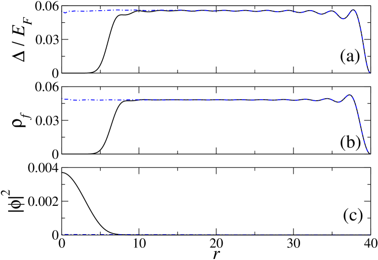
Figure 1: (Color online) Self-localization of ²³Na atoms in a superfluid mixture of ⁴⁰K atoms. Panel (a) shows the pairing function $\Delta(r)$, panel (b) fermion density $\rho_{f}(r)$ and panel (c) density of bosons $|\phi(r)|^{2}$. Solid black lines correspond to boson-fermion interaction strength $g_{bf}=10$ and dotted-dashed blue lines to $g_{bf}=0$. In panel (c) the dotted-dashed blue line is hardly visible because for $g_{bf}=0$ bosons are delocalized and their density very small. Number of bosons $N_{b}=100$ and fermions $N_{f}\approx 12000$ (chemical potential $\mu=E_{F}$) and fermion-fermion coupling constant $g_{ff}=-5.5$.

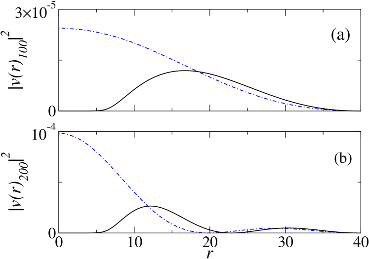
Figure 2: (Color online) Probability densities $|v_{nlm}(r)|^{2}$ of two fermion pairs at the bottom of the Fermi sea with angular momentum $l=0$. Panel (a) corresponds to the ground state ($n=1$) of the radial degree of freedom and panel (b) to the first excited state ($n=2$). Solid black lines correspond to boson-fermion interaction strength $g_{bf}=10$ and dotted-dashed blue lines to $g_{bf}=0$. All parameters are the same as in Fig. 1.

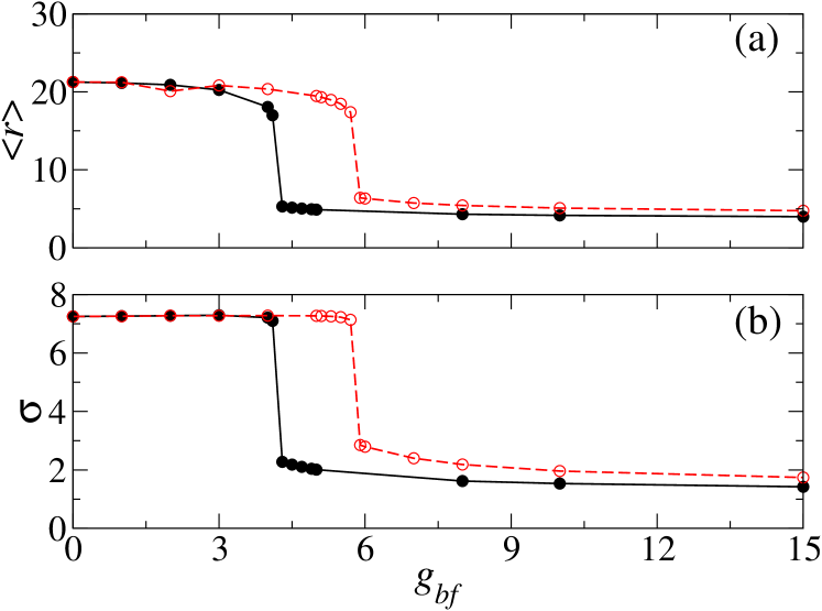
Figure 3: (Color online) The average radius of the Bose cloud $\langle r\rangle$ [panel (a)] and the standard deviation $\sigma=(\langle r^{2}\rangle-\langle r\rangle^{2})^{1/2}$ [panel (b)] versus boson-fermion coupling constant $g_{bf}$. Black full symbols correspond to a mixture of ²³Na and ⁴⁰K atoms while red open symbols to a mixture of ⁷Li and ⁴⁰K atoms. Note the abrupt transitions to localized states when critical values of $g_{bf}$ are reached. All the other parameters are the same as in Figs. 1-2.

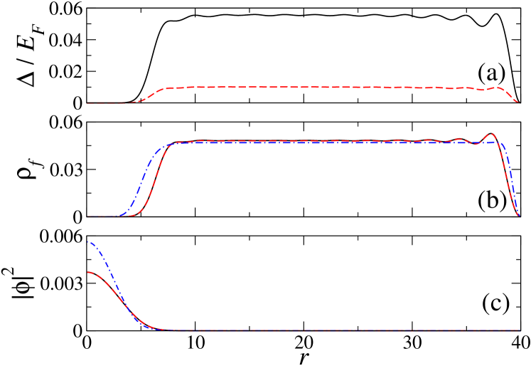
Figure 4: (Color online) Self-localization of ²³Na atoms in a superfluid mixture of ⁴⁰K atoms for non-zero temperature. Panel (a) shows the pairing function $\Delta(r)$, panel (b) fermion density $\rho_{f}(r)$ and panel (c) density of bosons $|\phi(r)|^{2}$. Solid black lines correspond to $T=0$ and $\mu=E_{F}$, red dashed lines to $T=0.028T_{F}$ and $\mu=E_{F}$, blue dotted-dashed lines to $T=6T_{F}$ and $\mu=0.16E_{F}$. Boson-fermion interaction strength $g_{bf}=10$, fermion-fermion coupling constant $g_{ff}=-5.5$ and number of bosons $N_{b}=100$ and fermions $N_{f}\approx 12000$. In panel (a) the dotted-dashed blue line is not visible because for $T=6T_{F}$ the pairing function is equal zero. In panels (c) and (d) the solid black and dashed red lines are hardly distinguishable.

Figure 1 shows the densities of bosons and fermions and the pairing function corresponding to the ground state of the system for $g_{bf}=0$ and $g_{bf}=10$. Without boson-fermion interactions the quantities are flat and uniform (except a small region close to the edge of the 3D volume due to assumed open boundary conditions). However, when the considerable interactions are turned on it becomes energetically favorable to separate bosons and fermions, the $\rho_{f}(\mathbf{r})$ is depleted around the center and bosons form a bound state localized in small area around $\mathbf{r}=0$. It is clear, that the localization effect is the result of boson-fermion interactions. It relies on a local deformation of the density of fermions and is not affected by the boundary conditions.

The response of the Fermi sub-system to bosons, that tend to localize, can be investigated by monitoring deformation of the Bogoliubov quasi-particle modes. The density of fermions is the sum of the Bogoliubov modes $\rho_{f}(\mathbf{r})=2\sum_{nlm}|v_{nlm}(\mathbf{r})|^{2}$. The modes with zero angular momentum contribute only to the density around $\mathbf{r}=0$. Consequently, the modification of these modes is primarily responsible for preparation of the potential well in which bosons localize. In Fig. 2 we illustrate the deformation of two modes with $l=0$ corresponding to fermions at the bottom of the Fermi sea but we should keep in mind that all modes with $l=0$ become affected by the interactions with bosons. The deformation of modes for fermions at the Fermi level is reflected by a change of a shape of the pairing field visible in Fig. 1, because those modes contribute mainly to $\Delta(\mathbf{r})$.

The interaction of fermions and the impurity Bose particles influences the pairing function $\Delta$ only locally, see Fig. 1. It implies that the superfluidity is not destroyed even when the interaction is so strong that the localization of the impurity object takes place.

The data in Figs. 1-2 are related to $N_{b}=100$ ²³Na atoms and the mixture of $N_{f}\approx 12000$ ⁴⁰K atoms (chemical potential $\mu=E_{F}$) in two different hyperfine states. We set the scattering lengths $g_{ff}=-5.5$ and $g_{bf}=10$ with the assumption that they can be realized by the use of the Feshbach resonances (e.g. magnetic resonance for fermions and optical resonance between bosons and fermions varonna2006 ; theis2004 ). In Fig. 3 we show the average radius of the Bose cloud $\langle r\rangle$ and the standard deviation $\sigma=(\langle r^{2}\rangle-\langle r\rangle^{2})^{1/2}$ as a function of the coupling constant $g_{bf}$. The self-localization means that both $\langle r\rangle$ and $\sigma$ are much smaller than the radius of the 3D volume. One can see that there is a critical non-zero value of $g_{bf}$ leading to the self-localization. This critical $g_{bf}$ is different from the critical value for the instability of the homogeneous solution (i.e. phase separation condition). The latter, for the case without boson-boson interactions, corresponds to $g_{bf}>0$. If we replace the sodium atoms by ⁷Li atoms, it turns out that the critical value of $g_{bf}$ for the self-localization increases. This is, because compressing the cloud of light lithium particles costs more energy than in the case of heavier sodium atoms.

A small non-zero temperature mostly affects superfluidity and has little effect on the self-localization phenomenon. Indeed, in Fig. 4 we see that even for $T=0.028T_{F}$ when the pairing function is very small the densities of bosons and fermions hardly change. Increasing temperature to $T=T_{F}$ (which is still much smaller than critical temperature for Bose-Einstein condensation of $N_{b}=100$ bosonic atoms localized in a volume of the radius $\langle r\rangle\approx 4$, i.e. $T_{\rm BEC}\approx 6T_{F}$) we observe effects of thermal fluctuations in the fermion density and a modification of the density of bosons but the self-localization persists. Thus, bosons self-localize both for the normal and superfluid phase of the Fermi sub-system.

We have considered the repulsive boson-fermion interaction. For the attractive interaction we do not observe the self-localization regardless on the phase of the Fermi sub-system. For $g_{bf}<0$ the particle densities may collapse to Dirac-delta distributions. For sufficiently small $|g_{bf}|$ a metastable state may appear. However, it turns out that the existence of such a metastable state is not the result of self-localization in the system. Indeed, it is an effect of a compromise between the requirement of minimal kinetic energies and restrictions related to the boundary conditions. In the following we consider a 1D model where there is no problem with the collapse of the densities and show that Bose particles can localize in the Fermi sub-system for attractive boson-fermion interactions too.

III.2 One dimensional model

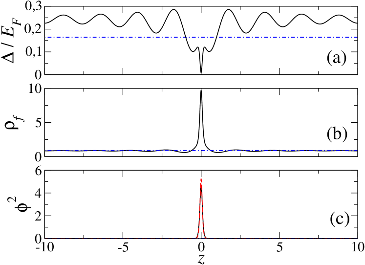
Figure 5: (Color online) Self-localization of a single boson ($N_{b}=1$) in a superfluid mixture of fermions in 1D space. Panel (a) shows the pairing function $\Delta(z)$, panel (b) fermion density $\rho_{f}(z)$ and panel (c) boson density $|\phi(z)|^{2}$. Solid black lines correspond to boson-fermion interaction strength $g_{bf}=-20$ and dotted-dashed blue lines to $g_{bf}=0$. Number of fermions $N_{f}\approx 20$ (chemical potential $\mu=E_{F}$) and fermion-fermion coupling constant $g_{ff}=-1$. Ratio of masses of Bose and Fermi particles $\frac{m_{b}}{m_{f}}$ fulfills Eq. (25). The configuration space extends from $z=-10$ to $z=10$. In panel (c) the dotted-dashed blue line is hardly visible, because the boson is delocalized and its density very small for $g_{bf}=0$. Red dashed line in panel (c) indicates the solitonic solution Eq. (26).

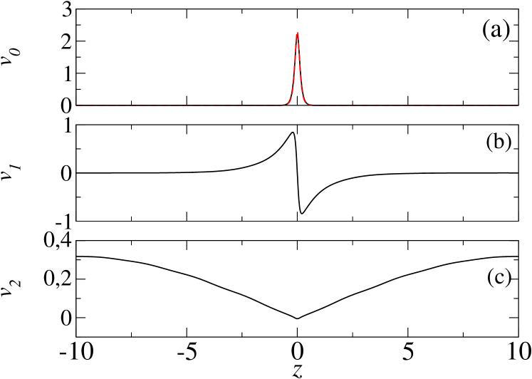
Figure 6: (Color online) Bogoliubov modes $v_{k}(z)$ corresponding to fermion pairs located close to the bottom of the Fermi sea. Panel (a) is related to the pair of fermions at the bottom of the Fermi sea, panel (b) and (c) to the next pairs. Solid black lines correspond to the numerical solutions. Red dashed line in panel (a) indicates solitonic solution Eq. (26). All the others parameters are the same as in Fig. 5.

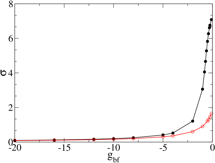
Figure 7: (Color online) Width of the boson density, i.e. $\sigma=(\langle z^{2}\rangle-\langle z\rangle^{2})^{1/2}$, versus boson-fermion coupling constant $g_{bf}$. Black full symbols correspond to the numerical values and red open symbols to the solutions Eq. (26). The configuration space extends from $z=-20$ to $z=20$. All the others parameters are the same as in Fig. 5.

If in $x$ and $y$ directions we apply harmonic potentials of frequency $\omega_{\perp}$ and $\hbar\omega_{\perp}$ is much greater than the chemical potentials, the 3D system becomes effectively one-dimensional. Then, the description reduces to the 1D version of Eqs. (5)-(13) with the following coupling constants [in the units (14)]

$$g_{ff}^{\rm 1D} = \frac{2m_{f}\omega_{\perp}}{\hbar k_{F}}a_{ff},$$ (19)

$$g_{bf}^{\rm 1D} = \frac{2m_{f}\omega_{\perp}}{\hbar k_{F}}a_{bf},$$ (20)

which have been obtained assuming that the $x$ and $y$ degrees of freedom of each atom are in the ground states of the harmonic potentials. In the 1D case there is no ultraviolet divergence and the pairing function does not require regularization. Nevertheless numerical simulations converge much faster if the Bogoliubov modes, above a numerical cut-off energy $E_{c}$, are included in the spirit of the local density approximation. That is, the coupling constant in $\Delta$ is substituted by

$$\frac{1}{|g_{\rm eff}^{\rm 1D}|}=\frac{1}{|g_{ff}^{\rm 1D}|}-\frac{1}{2\pi}\ln\frac{\sqrt{E_{C}}+\sqrt{\mu}}{\sqrt{E_{C}}-\sqrt{\mu}}.$$ (21)

For repulsive boson-fermion interactions, we observe the self-localization of bosons with the behaviour of the particle densities similar as in the 3D case. Therefore we focus on attractive interactions only. Figure 5 shows the results for $g_{bf}=-20$, obtained with periodic boundary conditions for fermions and open boundary conditions for bosons. For the attractive interactions bosons and fermions try to stick together which leads to an increase of the fermion density in the vicinity of the boson concentration and the creation of a potential well for localization of Bose particles.

Analyzing the Bogoliubov modes $v_{k}(z)$ (see Fig. 6) we find out that the probability density $v_{0}^{2}(z)$ of a pair of fermions at the bottom of the Fermi sea becomes strongly localized. The Bogoliubov mode $v_{1}(z)$ of the next fermion pair forms also a bound state. Since $v_{1}(z)$ is an antisymmetric function it is nearly zero in the area around $z=0$. Probability densities of other fermions are deformed and almost all of them drop to zero in the region where $v_{0}(z)$ is localized. This may be interpreted as a realization of the Pauli exclusion rule. In the BCS limit only particles close to the Fermi level contribute to the pairing function $\Delta$ and there is practically no contributions from fermions located deeply in the Fermi sea. Therefore there is also no contribution from the pair of fermions at the bottom of the Fermi sea. That is why $\Delta(z)$, contrary to the fermion density, reveals a minimum at $z=0$, see Fig. 5.

The analysis of the Bogoliubov modes suggests a simple model of self-localization in the case of attractive boson-fermion interactions. Suppose, that in the vicinity of the localized bosons we may neglect the pairing field and the density of all fermions except a fermion pair at the bottom of the Fermi sea. Then, we obtain the following set of equations

$$(\mu-E_{0})v_{0} = \left[-\frac{1}{2}\partial^{2}_{z}-|g_{ff}|v_{0}^{2}-|g_{bf}|N_{b}\phi^{2}\right]v_{0},$$ (22)

$$\mu_{b}\phi = \left[-\frac{m_{f}}{2m_{b}}\partial^{2}_{z}-2|g_{bf}|v_{0}^{2}\right]\phi.$$ (24)

For

$$\frac{m_{b}}{m_{f}}=\frac{N_{b}}{2}+\frac{|g_{ff}|}{2|g_{bf}|},$$ (25)

there exists analytical solution of Eqs. (22)-(24),

$$\phi(z)=v_{0}(z)=\sqrt{\frac{\alpha}{2}}\;{\rm sech}(\alpha z),$$ (26)

with

$$\alpha = |g_{bf}|\frac{m_{b}}{m_{f}},$$ (27)

$$E_{0} = \mu+\frac{g_{bf}^{2}m_{b}^{2}}{2m_{f}^{2}},$$ (28)

$$\mu_{b} = -\frac{g_{bf}^{2}m_{b}}{2m_{f}}.$$ (29)

Such a solution resembles vector solitons. They appear in non-linear optics when interactions of several field components are described by a set of coupled non-linear Schrödinger equations Kivshar . Note that for the self-localization of an impurity atom in a large BEC considered in Ref. Sacha2006 , the 1D system is described by a parametric soliton with the state of the impurity atom given by the hyperbolic secant squared function.

A comparison of the analytical solutions (26) with numerical results of the full set of equations is shown in Figs. 5-6. The agreement is very good and increases with the strength of boson-fermion interactions. Indeed, for the strong interaction, due to the Pauli exclusion rule, there is negligible probability density to find other fermions than the localized pair in the vicinity of $z=0$. As a consequence, the localized bosons interact almost exclusively with the localized fermion pair and the set of Eqs. (22)-(24) becomes exact.

Figure 6b shows that the Bogoliubov mode $v_{1}(z)$ forms an antisymmetric bound state. In the vicinity of $z=0$ (where the fermion density is dominated by $v_{0}^{2}$ and the pairing function drops to zero) this mode should fulfill equation similar to Eq. (22), that is

$$(\mu-E_{1})v_{1}=\left[-\frac{1}{2}\partial^{2}_{z}-|g_{ff}|v_{0}^{2}-|g_{bf}|N_{b}\phi^{2}\right]v_{1}.$$ (30)

If $\phi$ and $v_{0}$ are given by Eq. (26) the antisymmetric solution of Eq. (30) forms a marginal bound state

$$v_{1}(z) \sim \tanh(\alpha z),$$ (31)

$$E_{1} = \mu.$$ (32)

In the full description of the system, the state govern by the equation (19) may become either truely bound or unbound. In the considered system, it turns out that the state is pushed towards a true bound state as visible in Fig. 6b.

When the boson-fermion coupling constant $g_{bf}$ is decreased, we observe the increasing discrepancy between analytical and numerical solutions, see Fig. 7. The width of the boson probability density obtained numerically is significantly greater than the corresponding analytical value. This is due to the fact, that in the effective potential experienced by the bosons a considerable contribution comes from other fermions, and not only from the pair at the bottom of the Fermi sea. The density of such fermions, contrary to the localized fermion pair, possesses a minimum at $z=0$ and thus effectively makes the potential well for bosons weaker. Consequently, bosons occupy a much larger space than can be expected on the basis of solutions Eq. (26).

IV Conclusions

We have considered a small number of bosons immersed in a superfluid mixture of fermions in two different spin states. With negligible boson-boson interactions, homogeneous densities of the particles become unstable as soon as the boson-fermion coupling constant is non-zero. It corresponds to the phase separation transition. We show that in 3D space for sufficiently strong repulsive boson-fermion interactions another transition takes place, i.e. the self-localization of Bose particles. That is, the repulsion between particles creates a local potential well for bosons where, if the well is sufficiently large, they can localize. The self-localization is present both for the superfluid and the normal state of fermions. It modifies properties of the Fermi sub-system locally without destroying the superfluidity. Low non-zero temperature affects the pairing function but has little effect on the self-localization phenomenon.

We do not observe the self-localization for attractive boson-fermion interactions in the 3D case. In this context the self-localization requires sufficiently strong boson-fermion interactions. However, for strong attractive interactions no metastable state of the system exists and the densities of the atoms collapse to Dirac-delta distributions indicating a breakdown of the description with the contact interaction potentials. In the 1D case there is no collapse for attractive boson-fermion interactions. The self-localization of bosons is accompanied by localization of a pair of fermions at the bottom of the Fermi sea. This phenomenon can be described by a simple model where the self-localization is related to the existence of a vector soliton solution.

To realize experimentally the self-localization of bosons in a Fermi system, ultra-cold clouds of bosons and fermions have to be prepared in a laboratory. For a sufficiently large boson-fermion coupling constant, that can be achieved by means of a Feshbach resonance, the self-localization takes place. Signatures of the self-localization can be visible in expansion of the atomic clouds after trapping potentials are turned off. That is, if during the time of flight the boson-fermion interactions are kept negligibly weak, the initially strongly localized boson cloud will show much faster expansion than the Fermi cloud due to release of a large kinetic energy. The simplest experiment would employ a Fermi sub-system in a normal phase. In order to observe the self-localization in a superfluid Fermi mixture a manipulation of a fermion-fermion coupling constant is also needed and two Feshbach resonances must be employed, e.g. one resonance controlled by magnetic field and the other by optical means.

References

- (1)
- (2) M. Lewenstein, A. Sanpera, V. Ahufinger, B. Damski, A. Sen, and U. Sen, Adv. Phys. 56, 243 (2007).
- (3) I. Bloch, J. Dalibard, and W. Zwerger, Rev. Mod. Phys. 80, 885 (2008).
- (4) M. Greiner, O. Mandel, T. Esslinger, Th. W. Hänsch, and I. Bloch, Nature 415, 39 (2002).
- (5) L. Fallani, J. E. Lye, V. Guarrera, C. Fort, and M. Inguscio, Phys. Rev. Lett. 98, 130404 (2007).
- (6) J. Billy, V. Josse, Z. C. Zuo, A. Bernard, B. Hambrecht, P. Lugan, D. Clement, L. Sanchez-Palencia, P. Bouyer, A. Aspect, Nature 453, 891 (2008).
- (7) G. Roati, C. D’Errico, L. Fallani, M. Fattori, C. Fort, M. Zaccanti, G. Modugno, M. Modugno, M. Inguscio, Nature 453, 895 (2008).
- (8) C. A. Regal, M. Greiner, and D. S. Jin, Phys. Rev. Lett. 92, 040403 (2004).
- (9) M. Inguscio, W. Ketterle, and C. Salomon (Editors), Ultra-cold Fermi Gases, Proceedings of the International School of Physics “Enrico Fermi,” Course CLXIV, Varenna 2006, (IOS Press, Amsterdam) 2007.
- (10) R. M. Kalas and D. Blume, Phys. Rev. A 73, 043608 (2006).
- (11) F. M. Cucchietti and E. Timmermans, Phys. Rev. Lett. 96, 210401 (2006).
- (12) K. Sacha and E. Timmermans, Phys. Rev. A 73, 063604 (2006).
- (13) M. Bruderer, W. Bao, and D. Jaksch, Europhys. Lett. 82, 30004 (2008).
- (14) M. Bruderer, A. Klein, S. R. Clark, and D Jaksch, New J. Phys. 10 033015 (2008).
- (15) D. H. Santamore, and Eddy Timmermans, Phys. Rev. A 78, 013619 (2008).
- (16) D. C. Roberts and S. Rica, Phys. Rev. Lett. 102, 025301 (2009).
- (17) A. Novikov and M. Ovchinnikov, J. Phys. A: Math. Theor. 42, 135301 (2009).
- (18) J. Tempere, W. Casteels, M. K. Oberthaler, S. Knoop, E. Timmermans, and J. T. Devreese, Phys. Rev. B 80, 184504 (2009).
- (19) A. Novikov and M. Ovchinnikov, J. Phys. B: At. Mol. Opt. Phys. 43, 105301 (2010).
- (20) G. D. Mahan, Many-Particle Physics, Plenum Press, New York 1981.
- (21) F. Chevy, Phys. Rev. A 74, 063628 (2006).
- (22) R. Combescot, A. Recati, C. Lobo, and F. Chevy, Phys. Rev. Lett. 98, 180402 (2007).
- (23) M. Punk and W. Zwerger, Phys. Rev. Lett. 99, 170404 (2007).
- (24) N. V. Prokofev, and B. V. Svistunov, Phys. Rev. B 77, 020408(R) (2008).
- (25) N. V. Prokofev, and B. V. Svistunov, Phys. Rev. B 77, 125101 (2008).
- (26) M. Punk, P. T. Dumitrescu, and W. Zwerger, Phys. Rev. A 80, 053605 (2009).
- (27) A. Schirotzek, C.-H. Wu, A. Sommer, and M. Zwierlein, Phys. Rev. Lett. 102, 1 (2009).
- (28) S. Nascimbene, N. Navon, K. J. Jiang, L. Tarruell, M. Teichmann, J. McKeever, F. Chevy, and C. Salomon, Phys. Rev. Lett. 103, 170402 (2009).
- (29) K. Mølmer, Phys. Rev. Lett. 80, 1804 (1998).
- (30) L. Viverit, C. Pethick, and H. Smith, Phys. Rev. A 61, 1 (2000).
- (31) S. Yip, Phys. Rev. A 64, 2 (2001).
- (32) R. Roth, Phys. Rev. A 66, 1 (2002).
- (33) H. Pu, W. Zhang, M. Wilkens, and P. Meystre, Phys. Rev. Lett. 88, 5 (2002).
- (34) S. Adhikari and L. Salasnich, Phys. Rev. A 76, 1 (2007).
- (35) S. Bhongale and H. Pu, Phys. Rev. A 78, 1 (2008).
- (36) D.-S. Lühmann, K. Bongs, K. Sengstock, and D. Pfannkuche, Phys. Rev. Lett. 101, 1 (2008).
- (37) Yu-Li Lee and Yu-wen Lee, arXiv:0910.0603.
- (38) B. Ramachandhran, S. G. Bhongale and H. Pu, arXiv:0911.2487.
- (39) M. S. Mashayekhi, J. L. Song, F. Zhou, arXiv:1003.3096.
- (40) T. Karpiuk, M. Brewczyk, S. Ospelkaus-Schwarzer, K. Bongs, M. Gajda, and K. Rza̧żewski, Phys. Rev. Lett. 93, 100401 (2004).
- (41) T. Karpiuk, M. Brewczyk, and K. Rza̧żewski, Phys. Rev. A 73, 053602 (2006).
- (42) S. K. Adhikari, Phys. Rev. A 72, 053608 (2005).
- (43) G. Bruun, Y. Castin, R. Dum, and K. Burnett, Eur. Phys. J. D 7, 433 (1999).
- (44) A. Bulgac and Y. Yu, Phys. Rev. Lett. 88, 042504 (2002).
- (45) M. Grasso and M. Urban, Phys. Rev. A 68, 033610 (2003).
- (46) A. Niederberger, J. Wehr, M. Lewenstein, and K. Sacha, Europhys. Lett. 86 26004 (2009).
- (47) M. Theis, G. Thalhammer, K. Winkler, M. Hellwig, G. Ruff, R. Grimm, and J. Hecker Denschlag, Phys. Rev. Lett. 93, 123001 (2004).
- (48) Y. S. Kivshar and G. P. Agrawal, Optical Solitons, Academic Press, An imprint of Elsevier Science, San Diego, California, 2003.