Dynamics of periodic second-order equations between an ordered pair of lower and upper solutions

Abstract

We consider periodic second-order equations having an ordered pair of lower and upper solutions and show the existence of asymptotic trajectories heading towards the maximal and minimal periodic solutions which lie between them.

Key words: Lower and upper solutions, dynamics, asymptotic solutions, instability.

1 Introduction

Let $f=f(t,u,\dot{u})$ be $T$-periodic in time and consider the second-order equation

$$-\ddot{u}=f(t,u,\dot{u})\,.$$ (1)

A well-known strategy to find $T-$periodic solutions is the so-called lower and upper solutions method. Roughly speaking, this approach requires finding periodic functions $\alpha\leq\beta$ with $-\ddot{\alpha}\leq f(t,\alpha,\dot{\alpha})$ and $-\ddot{\beta}\geq f(t,\beta,\dot{\beta})$, and under some conditions on the dependence of $f$ with respect to $\dot{u}$, it guarantees the existence of some periodic solution $x$ between them.

As a model, we may think on the $T$-periodic problem for the damped pendulum equation:

$$-\ddot{u}=c\,\dot{u}+a\sin u\,,$$ (2)

where $c\geq 0$ and $a>0$ are given parameters. We observe that

$$\alpha(t)\equiv\frac{\pi}{2}\,,\hskip 56.9055pt\beta(t)\equiv\frac{3\pi}{2}$$

are, respectively, lower and upper solutions. They enclose the $T-$periodic solution $x(t)\equiv\pi$, which is unstable. Moreover, this equation possesses other solutions which are asymptotic to $x$; infinitely many in the past and also infinitely many in the future.

A second look at this example shows that

$$\hat{\alpha}(t)\equiv\frac{\pi}{2}-2\pi\,,\hskip 56.9055pt\hat{\beta}(t)\equiv\frac{3\pi}{2}+2\pi$$

also make up an ordered pair of lower and upper solutions. This time there are several periodic solutions, with different dynamics, between them. For instance, $x(t)\equiv 0$ is stable in the future (throughout this paper stability is understood in the the Lyapunov sense) . But the minimal and the maximal periodic solutions of (2) which lie between $\hat{\alpha}$ and $\hat{\beta}$ are, respectively,

$$x_{\min}(t)\equiv-\pi\,,\hskip 56.9055ptx_{\max}(t)\equiv 3\pi\,,$$

and both of them are unstable (we call instability to the logical negation of Lyapunov stability). Indeed, both $x_{\min}$ and $x_{\max}$ are again the limit of infinitely many asymptotic solutions.

In this paper we generalize this fact for more general equations (1) having an ordered pair $\alpha\leq\beta$ of periodic lower and upper solutions. Assuming that, for instance, $\alpha$ does not solve our equation (1) we show that the minimal periodic solution $x_{\min}$ lying between $\alpha$ and $\beta$ is unstable; moreover, it is the limit of many asymptotic solutions, in the past and in the future (Theorem 3.1 and Corollary 3.2). Of course, a similar statement holds for the maximal periodic solution $x_{\max}$ if $\beta$ does not solve (1).

This result raises the question about the case in which $\alpha<\beta$ are ordered $T-$periodic solutions of our equation (1). Is it still possible to find an unstable solution between them? The answer is affirmative in the conservative case $-\ddot{u}=f(t,u)$ (Corollary 4.4). For general, derivative-depending equations it may not true, but we shall see that when the periodic solutions are neighboring, then one of them must be unstable and possess many asymptotic solutions (Theorem 4.1 and Corollary 4.2).

The instability of the periodic solutions obtained by the method of lower and upper solutions was previously studied by Dancer and Ortega [1]. When the lower and upper solutions are strict and the number of periodic solutions between them is finite, they showed that at least one of them must be unstable. This result was obtained as an application of a general theorem on the index of stable fixed points in two dimensions whose proof depended on a nonelementary result of planar topology: Brouwer’s lemma on translation arcs.

Even though the main result of this paper can be seen as a generalization of Proposition 3.1 of [1], our approach, which is inspired on the Aubry-Mather theory as presented by Moser [5], is based on the more elementary concepts of maximal and minimal solutions of Dirichlet and periodic boundary value problems. Moreover, we do not need to assume the finiteness of the set of periodic solutions comprised between the lower and upper solutions and we shall obtain more precise information on the dynamics: the existence of branches of asymptotic solutions.

This paper is distributed in five sections. In Section 2 we make precise the framework which we shall use and collect some basic facts on upper and lower solutions which will be needed in the proofs. We do not pretend any originality in this section, whose contents are mostly well-known in slightly different frameworks. To keep the pace of the exposition, the proofs of these results will be postponed to the Appendix (Section 5). The main results of this paper are stated and proved in Sections 3 (where we study the dynamics between an ordered pair of lower and upper solutions) and 4 (devoted to the dynamics between two ordered solutions).

Some remarks on the notation (previously employed). Through most of the paper the Greek letters $\alpha$ and $\beta$ will be kept, respectively, for lower and upper solutions; however, in Section 4 they will represent two ordered periodic solutions. We shall also utilize different notations to distinguish solutions depending on the kind of boundary conditions that they satisfy. In this way, periodic solutions will be usually written as $x$, the letter $y$ will be used to emphasize that our solution satisfies some Dirichlet conditions, and $u$ will stand for other solutions, not necessarily verifying any particular boundary condition. Finally, it will be convenient to adopt the following convention: given functions $h_{1},h_{2}$ defined on respective domains $I_{1},I_{2}\subset\mathbb{R}$, and some set $J\subset I_{1}\cap I_{2}$, we shall simply say $h_{1}\leq h_{2}$ (resp., $h_{1}<h_{2}$) on $J$ instead of $h_{1}(t)\leq h_{2}(t)$ (resp., $h_{1}(t)<h_{2}(t)$) for any $t\in J$. When there is no possible ambiguity on the domain we shall say $h_{1}\leq h_{2}$ or $h_{1}<h_{2}$ meaning that the inequality holds pointwise. Given functions $u,v,w:I\to\mathbb{R}$ we shall say that $w$ lies between $u$ and $v$ on $I$ to mean $u\leq w\leq v$ on $I$.

It was shown in [9] that periodic minimizers are unstable. I am indebted to Prof. P. Omari for pointing out to me that it implies the instability of periodic solutions given by the lower and upper solutions method when the problem has a variational structure and formulating the question about the nonvariational case.

Last but not least, I want to express my gratitude to Prof. R. Ortega directing me to Moser’s book [5], as well as for his invaluable advice on many aspects of this paper, including the regularity result on lower and upper solutions described in the Appendix.

2 Some basic facts on lower and upper solutions

In this paper, the nonlinearity $f:\mathbb{R}^{3}\to\mathbb{R}$, $(t,u,\dot{u})\mapsto f(t,u,\dot{u})$ will always be assumed to be continuous and $T$-periodic in time. The function $\alpha:\mathbb{R}\to\mathbb{R}$ is called a lower solution of the periodic problem

$$(P)\equiv\begin{cases}-\ddot{x}=f(t,x,\dot{x})\,,\vspace{0.3cm}\\ x(t)=x(t+T)\ \text{ for any }t\in\mathbb{R}\,.\end{cases}$$

provided that it is Lipschitz-continuous and $T$-periodic, and verifies the inequality

$$-\ddot{\alpha}\leq f(t,\alpha,\dot{\alpha})\,,$$ (3)

in the distributional sense on the real line. With other words,

$$\int_{-\infty}^{\infty}\dot{\alpha}(t)\dot{\varphi}(t)\,dt\leq\int_{-\infty}^{\infty}f(t,\alpha(t),\dot{\alpha}(t))\varphi(t)\,dt\,,$$ (4)

for any nonnegative $\varphi\in\mathcal{C}^{\infty}(\mathbb{R})$ having compact support. Upper solutions $\beta$ are defined similarly after changing the sign of inequalities (3,4).

Of course, if $\alpha$ is a $\mathcal{C}^{2}$ function, then (4) is equivalent to (3) holding pointwise. But the definition above includes also some functions displaying angles. We point out an example which will be used later. Let $\alpha:[0,T]\to\mathbb{R}$ be a solution of our equation (1) such that $\alpha(0)=\alpha(T)$ but $\dot{\alpha}(0)>\dot{\alpha}(T)$, and extend it to the real line by periodicity. The resulting, piecewise $\mathcal{C}^{2}$ function, is a lower solution of $(P)$, as one may easily check using an integration-by-parts argument.

Notice also that our concepts of lower and upper solutions are nonstrict; periodic solutions are examples of lower and upper solutions.

The distributional notion of lower and upper solutions adopted in this paper is routinely used in PDE problems but may seem unnecessarily general here. Indeed, our main arguments could be carried out using only piecewise-$\mathcal{C}^{2}$ lower and upper solutions, even though the results obtained in this way would lose some generality. Our choice will imply some relatively small variations with respect to other versions in the literature when showing the results of this Section, but otherwise it will not lead to additional difficulties in the proofs. Incidentally we observe that lower and upper solutions in the distributional sense must be somewhat more regular than merely Lipschitz-continuous; for instance, the derivative should have side limits at each point (it will be shown in the proof of Lemma 2.7 in the Appendix).

If $f=f(t,u)$ does not depend on $\dot{u}$, then the existence of an ordered pair $\alpha\leq\beta$ of lower and upper solutions for $(P)$ implies the existence of a solution between them. However, this result fails to hold for general, derivative-dependent nonlinearities as considered in this paper, see [2], Example 4.1, pp. 43-44. To ensure that the method of lower and upper solutions works for $(P)$ one must add some further condition, which may consist on a special form of our equation (the Rayleigh equation, the Liénard equation…) or some assumption on the growth of $f$ with respect to $\dot{u}$ (such as the Bernstein condition or some kind of Nagumo condition); see [2], Chapter I, Section 4 for a detailed study of all these possibilities. In this paper we opt for the classical, two-sided Nagumo condition:

1. There exists a continuous function $\varphi:[0,+\infty)\to(0,+\infty)$ with

   $$\int_{0}^{+\infty}\frac{v}{\varphi(v)}\,dv>\max_{\mathbb{R}}\beta-\min_{\mathbb{R}}\alpha\,,$$

   and such that $|f(t,u,\dot{u})|\leq\varphi(|\dot{u}|)$ if $\alpha(t)\leq u\leq\beta(t)\,.$

This assumption makes the usual existence result for the periodic method of lower and upper solutions hold:

Proposition 2.1 (Upper and lower solutions method for periodic problems).

Let $(P)$ have an ordered pair $\alpha\leq\beta$ of lower and upper solutions and assume [N]. Then there exists a solution $x$ of $(P)$ with $\alpha\leq x\leq\beta$.

Lower and upper solutions are nowadays standard notions, and have been studied in depth. We shall be particularly interested on the structure of the set of solutions of $(P)$ lying between a given ordered pair $\alpha\leq\beta$ of lower and upper solutions. This set always contains a minimal and a maximal solution, and the following improvement of Proposition 2.1 is well-known:

Proposition 2.2.

Let $(P)$ have an ordered pair $\alpha\leq\beta$ of lower and upper solutions and assume [N]. Then there are solutions $x_{\min},\ x_{\max}$ of $(P)$ with

$$\alpha\leq x_{\min}\leq x_{\max}\leq\beta\,,$$

and such that any third solution $x$ of $(P)$ with $\alpha\leq x\leq\beta$ verifies

$$x_{\min}\leq x\leq x_{\max}\,.$$

Since the dependence of $f$ with respect to $(u,\dot{u})$ was only required to be continuous, initial value problems associated to our equation (1) may have many periodic solutions. Sometimes we shall merely look for global branches of asymptotic solutions to a given periodic motion and it will be not problematic. But other results of this paper explicitly deal with the instability of certain periodic solutions; in these cases, uniqueness for initial value problems will be assumed in combination with [N]. We emphasize a connection between these assumptions and the method of lower and upper solutions:

Proposition 2.3.

Assume that there is uniqueness for initial value problems associated to (1) and $\alpha\leq\beta$ are lower and upper solutions of $(P)$. Finally, assume also [N]. Then either $\alpha(t)<\beta(t)$ for any $t\in\mathbb{R}$ or $\alpha\equiv\beta$.

Concerning this result we remark that the lower and upper solutions $\alpha,\beta$ are not assumed to be strict. In particular, it also applies when either $\alpha$ or $\beta$ are periodic solutions. We shall use this form of Proposition 2.3 in the proof of Corollary 3.2.

In this paper we shall also consider Dirichlet-type boundary value problems:

$$(D)\equiv\begin{cases}-\ddot{y}=f(t,y,\dot{y})\,,\vspace{0.3cm}\\ y(a)=y_{a}\,,\ \ y(b)=y_{b}\,,\end{cases}$$

where $a<b$ and $y_{a},y_{b}\in\mathbb{R}$ are given. By a lower solution to $(D)$ we mean a Lipschitz-continuous function $\alpha:[a,b]\to\mathbb{R}$ such that

$$\alpha(a)\leq y_{a},\hskip 56.9055pt\alpha(b)\leq y_{b}\,,$$ (5)

and (3) holds in the distributional sense on $(a,b)$. With other words, a Lipschitz-continuous function $\alpha$ verifying (5) and such that (4) holds for any nonnegative $\varphi\in\mathcal{C}^{\infty}(\mathbb{R})$ with compact support contained in $(a,b)$. Upper solutions $\beta$ for this problem are then defined similarly by changing the sign of the inequalities.

In this framework it is also well-known that the presence of an ordered pair of lower and upper solutions does not necessarily imply the existence of a solution between them. We might use a related Nagumo condition, but for the purposes of this paper it will suffice to consider the more restrictive class of nonlinearities which are bounded between $\alpha$ and $\beta$, i.e., there exists some constant $M>0$ such that

$$|f(t,u,\dot{u})|\leq M\ \ \text{ if }\alpha(t)\leq u\leq\beta(t)$$ (6)

for any $t\in[a,b]$.

Proposition 2.4 (Lower and upper solutions method for Dirichlet problems).

Let (D) have an ordered pair $\alpha\leq\beta$ of lower and upper solutions and let $f$ be bounded between them. Then there are solutions $y_{\min},\ y_{\max}$ of (D) with

$$\alpha\leq y_{\min}\leq y_{\max}\leq\beta\ \text{ on }[a,b]\,,$$

and such that any third solution $y$ of (D) with $\alpha\leq y\leq\beta$ on $[a,b]$ verifies

$$y_{\min}\leq y\leq y_{\max}\ \text{ on }[a,b]\,.$$

For solutions of Dirichlet problems, the quality of being minimal or maximal is inherited after restriction to a smaller interval. To state this result in a precise form, let us assume that $\alpha\leq\beta$ are ordered lower and upper solutions of $(D)$ and $y:[a,b]\to\mathbb{R}$ is a solution between them. Given $a\leq\tilde{a}<\tilde{b}\leq b$, the restriction of $y$ to $[\tilde{a},\tilde{b}]$ solves the Dirichlet problem

$$(\tilde{D})\equiv\begin{cases}-\ddot{y}=f(t,y,\dot{y})\,,\vspace{0.3cm}\\ y(\tilde{a})=\tilde{y}_{a}\,,\ \ y(\tilde{b})=\tilde{y}_{b}\,,\end{cases}$$

for suitable choices of $\tilde{y}_{a}$ and $\tilde{y}_{b}$. Also, the restrictions of $\alpha$ and $\beta$ to $[\tilde{a},\tilde{b}]$ become lower and upper solutions for $(\tilde{D})$.

Proposition 2.5.

Let $f$ be bounded between $\alpha$ and $\beta$ and let $y$ be the minimal/maximal solution of $(D)$ lying between them. Then, $y_{\big{|}[\tilde{a},\tilde{b}]}$ is the minimal/maximal solution of ($\tilde{D}$) lying between ${\alpha}_{\big{|}[\tilde{a},\tilde{b}]}$ and ${\beta}_{\big{|}[\tilde{a},\tilde{b}]}$

We shall need also some facts on the relative compactness on the $\mathcal{C}^{2}$ topology of some sets of solutions of our equation. The next result is not directly related with the method of lower and upper solutions but follows from the boundedness assumption on $f$. To present it precisely, we choose numbers $a<b$ and assume that the sequence $u_{n}:[a,b]\to\mathbb{R}$ of solutions of (1) is uniformly bounded and pointwise converging. With other words,

$$\{u_{n}(t)\}_{n}\ \text{ converges for every }t\in[a,b]\,,\hskip 42.67912pt(t,u_{n}(t))\in\mathcal{B}\ \text{ for all }t\in[a,b]\text{ and }n\in\mathbb{N}\,,$$ (7)

where $\mathcal{B}$ is some compact region of $[a,b]\times\mathbb{R}$.

Proposition 2.6.

Assume that $f$ is bounded on $\mathcal{B}\times\mathbb{R}$ and $(\ref{eu9})$. Then, $u(t):=\lim_{n\to+\infty}u_{n}(t)$ is again a solution of $(\ref{eu0})$ and $\{u_{n}\}\to u$ in the $\mathcal{C}^{2}[a,b]$ topology. Precisely,

$$\lim_{n\to\infty}(u_{n}(t)-u(t))=0,\hskip 34.14322pt\lim_{n\to\infty}(\dot{u}_{n}(t)-\dot{u}(t))=0,\hskip 34.14322pt\lim_{n\to\infty}(\ddot{u}_{n}(t)-\ddot{u}(t))=0\,,$$

uniformly with respect to $t\in[a,b]$.

Some results of this paper will be first shown when the equation is bounded between a given pair $\alpha\leq\beta$ of periodic lower and upper solutions, i.e., assuming that (6) holds for some constant $M>0$. This assumption will be subsequently relaxed to [N] by replacing (1) with a modified equation

$$-\ddot{u}=\tilde{f}(t,u,\dot{u}) \tilde{1}$$ ()

which will be bounded between $\alpha$ and $\beta$ and share many periodic solutions with the original equation. For this reason, the next Lemma will be evoked several times throughout this paper.

Lemma 2.7 (Modification Lemma).

Let (P) have an ordered pair $\alpha\leq\beta$ of lower and upper solutions and assume [N]. Then, there exists some continuous and $T$-periodic in time $\tilde{f}:\mathbb{R}^{3}\to\mathbb{R}$ which is bounded between $\alpha$ and $\beta$ and verifies:

1. $\alpha$ and $\beta$ remain, respectively, lower and upper solutions for the $T$-periodic problem associated to $(\tilde{1})$.

2. Any solution $u:I\to\mathbb{R}$ of $(\tilde{1})$ for which $u-\alpha$ attains a local minimum at some interior point $t_{0}$ of $I$ satisfies $u(t_{0})\geq\alpha(t_{0})$. Similarly, given a solution $u:I\to\mathbb{R}$ of $(\tilde{1})$ such that $u-\beta$ attains a local maximum at some interior point $t_{0}$ of $I$ one has $u(t_{0})\leq\beta(t_{0})$.

3. There exists some $\epsilon>0$, not depending on $t_{0},u,$ nor the interval $I$, such that $(\ref{eu0})$ and $(\tilde{1})$ have exactly the same solutions $u:I\to\mathbb{R}$ with

   $$\alpha\leq u\leq\beta\text{ on }I\,,\hskip 56.9055pt|\dot{u}(t_{0})|<\epsilon\text{ for some }t_{0}\in I\,.$$

We notice the following consequence of (ii)-(iii): the periodic solutions of the modified equation $(\tilde{1})$ are the periodic solutions of the original equation $(1)$ lying between $\alpha$ and $\beta$. In particular, the maximal and the minimal $T$-periodic solutions between $\alpha$ and $\beta$ coincide for both equations.

The results described in this Section will be discussed with some detail in the Appendix. Next, we present and prove the main results of this paper.

3 Maximal or minimal periodic solutions and asymptotic trajectories

Our starting point will be the periodic problem $(P)$, which through this Section we assume to have an ordered pair $\alpha\leq\beta$ of lower and upper solutions. As usually, the solution $u_{r}:[0,+\infty)\to\mathbb{R}$ of (1) will be called asymptotic in the future to the periodic solution $x$ if

$$\lim_{t\to+\infty}\big{(}u_{r}(t)-x(t)\big{)}=\lim_{t\to+\infty}\big{(}\dot{u}_{r}(t)-\dot{x}(t)\big{)}=0\,.$$ (8)

Similarly, one may speak of solutions $u_{l}:(-\infty,0]\to\mathbb{R}$ which are asymptotic in the past to a given periodic solution.

Theorem 3.1.

Assume [N]. Assume also that, for instance, $\alpha$ is not a solution of $(P)$ and let $x_{\min}$ be the minimal solution of $(P)$ lying between $\alpha$ and $\beta$. Then, for any initial position

$$u_{0}\in\Big{[}\alpha(0),x_{min}(0)\Big{)}\,,$$

there are solutions $u_{l}:(-\infty,0]\to\mathbb{R},\ \ u_{r}:[0,+\infty)\to\mathbb{R}$ of (1) with

$$u_{l}(0)=u_{0}=u_{r}(0)\,,\hskip 36.98866pt\alpha\leq u_{l}\leq x_{\min}\ \text{ on }(-\infty,0]\,,\hskip 36.98866pt\alpha\leq u_{r}\leq x_{\min}\ \text{ on }[0,+\infty)\,,$$ (9)

which are asymptotic to $x_{\min}$ in the past and in the future respectively. See Fig. 1 below.

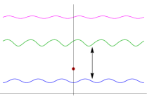
Figure 1: If $\alpha$ is not a solution, then $x_{\min}$ is the limit of many asymptotic solutions.

Remark: We recall that the (global) stable manifold of the periodic solution $x$ is the set $W^{S}(x)$ of initial conditions of solutions $u_{r}$ which are asymptotic to $x$ in the future:

$$W^{S}(x):=\Big{\{}\big{(}u_{r}(0),\dot{u}_{r}(0)\big{)}\text{ such that the solution }u_{r}:[0,+\infty)\to\mathbb{R}\text{ of }(\ref{eu0})\text{ satisfies }(\ref{eu17})\Big{\}}\,.$$

Similarly, the unstable manifold associated to $x$ is the set $W^{U}(x)$ of initial conditions of solutions $u_{l}$ which are asymptotic to $x$ in the past. These sets allow us to reformulate part of the information given by Theorem 3.1 as follows:

Theorem 3.1$.^{*}$Assume [N]. Assume also that $\alpha$ is not a solution of $(P)$, and let $x_{\min}$ be the minimal solution of $(P)$ lying between $\alpha$ and $\beta$. Then, for any initial position $u_{0}\in[\alpha(0),x_{\min}(0))$ there are initial velocities $v_{l},v_{r}\in\mathbb{R}$ such that

$$(u_{0},v_{l})\in W^{U}(x_{\min}),\hskip 56.9055pt(u_{0},v_{r})\in W^{S}(x_{\min})\,.$$

If $f$ satisfies some smoothness assumptions and the periodic solution $x$ is hyperbolic, then the Stable manifold Theorem states that $W^{U}(x)$ and $W^{S}(x)$ are injectively immersed smooth curves, see e.g. [8], Theorem 6.2. However, this result does not always apply to $x_{\min}$ under the assumptions of Theorem 3.1, because $x_{\min}$ may not be hyperbolic. Indeed, one may construct a periodic in time, $\mathcal{C}^{0,2}$ equation $-\ddot{x}=f(t,x)$ which is repulsive in the sense that

$$f(t,0)=0\,,\hskip 56.9055ptf(t,-x)>0>f(t,x)\ \forall x>0\,,$$ (10)

and such that the stable manifold $W^{S}(x_{*})$ associated to the periodic solution $x_{*}\equiv 0$ is pathological, see [10]. Observe that (10) implies that every negative constant is a lower solution of the associated periodic problem, every positive constant is an upper solution, and $x_{*}\equiv 0$ is the only periodic solution of the equation.

Proof of Theorem 3.1.

After replacing $t$ with $-t$ one observes that it suffices to prove the part of the statement concerning the solutions $u_{r}$ which are asymptotic to $x_{\min}$ in the future. The proof will be divided into two steps. Notice that Step 1 and Phase 2(a) assume the boundedness of $f$ between the lower and the upper solutions.

(Step 1) Let $f$ be bounded between $\alpha$ and $\beta$. Then, there exists some solution $u:[0,+\infty)\to\mathbb{R}$ which is asymptotic to $x_{\min}$ in the future and at initial time $t=0$ starts from the position $u_{0}=\alpha(0)$.

To show this Step we consider, for each $n\in\mathbb{N}$, the Dirichlet problem

$$(D_{n})\equiv\begin{cases}-\ddot{y}=f(t,y,\dot{y})\,,\vspace{0.3cm}\\ y(0)=\alpha(0)\,,\ \ y(nT)=x_{\min}(nT)\,.\end{cases}$$

Observe that $\alpha$ is a lower solution for this problem, while $x_{\min}$ is an upper solution. Furthermore $\alpha\leq x_{\min}$. Then, Proposition 2.4 states the existence of some solution of $(D_{n})$ which lies between $\alpha$ and $x_{\min}$. This solution may not be unique, but we choose the maximal one and call it $y_{n}$. In this way, $y_{n}$ is a $\mathcal{C}^{2}$ function on $[0,nT]$. We organize the proof of Step 1 in four phases:

(Phase 1a)                  $y_{n}(t-T)\leq y_{n}(t)\,,\hskip 56.9055ptt\in[T,nT]\,.$

To check this assertion we use a contradiction argument and assume instead that the contrary happens for some $t_{*}\in[T,nT]$. We denote $\tilde{y}_{n}(t):=y_{n}(t-T)$, which solves our equation on $[T,nT]$ and verifies:

$$\tilde{y}_{n}(T)\leq y_{n}(T)\,,\hskip 28.45274pt\tilde{y}_{n}(nT)\leq y_{n}(nT)\,,\hskip 28.45274pt\tilde{y}_{n}(t_{*})>y_{n}(t_{*})\,,$$

and this implies the existence of numbers $T\leq\tilde{a}<t_{*}<\tilde{b}\leq nT$ such that

$${\tilde{y}}_{n}(\tilde{a})=y_{n}(\tilde{a})\,,\hskip 56.9055pt{\tilde{y}}_{n}(\tilde{b})=y_{n}(\tilde{b})\,,$$

(see Fig. 2(a)). In view of Proposition 2.5, ${y_{n}}_{\big{|}[\tilde{a},\tilde{b}]}$ should be the maximal solution of the Dirichlet problem

$$(\tilde{D})\equiv\begin{cases}-\ddot{y}=f(t,y,\dot{y})\,,\vspace{0.3cm}\\ y(\tilde{a})=y_{n}(\tilde{a})\,,\ \ y(\tilde{b})=y_{n}(\tilde{b})\,.\end{cases}$$

But ${\tilde{y}_{n}}\hskip 28.45274pt_{\big{|}[\tilde{a},\tilde{b}]}$ also solves $(\tilde{D})$ and at time $t_{*}$ it is greater than $y_{n}$. This contradiction shows Phase 1a.

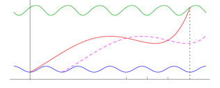
Figure 2: (a) The solutions $y_{n}$ must increase on time intervals of length $T$. (b) If $y_{n+1}$ is greater than $y_{n}$ at some point $t_{*}$, then $y_{n}$ is not maximal on the interval $[0,\tilde{b}]$.

(Phase 1b)                 $y_{n}\geq y_{n+1}\ \text{ on }[0,nT]\,.$

The proof of this new assertion uses similar ideas to the previous one. Since, should it fail to be true, we could find some time $t_{*}\in[0,nT]$ with $y_{n}(t_{*})<y_{n+1}(t_{*})$. But $y_{n}(nT)=x_{\min}(nT)\geq y_{n+1}(nT)$, and we deduce the existence of some $\tilde{b}\in(t_{*},nT]$ such that $y_{n}(\tilde{b})=y_{n+1}(\tilde{b})$, see Fig. 2(b).

Since furthermore $y_{n}(0)=\alpha(0)=y_{n+1}(0)$, Proposition 2.5 states that both ${y_{n}}_{\big{|}[0,\tilde{b}]}$ and ${y_{n+1}}_{\big{|}[0,\tilde{b}]}$ should be the maximal solution of the Dirichlet problem

$$(\tilde{D})\equiv\begin{cases}-\ddot{y}=f(t,y,\dot{y})\,,\vspace{0.3cm}\\ y(0)=\alpha(0)\,,\ \ y(\tilde{b})=y_{n}(\tilde{b})\,.\end{cases}$$

Hence, these solutions must be constantly equal, contradicting the existence of $t_{*}$.

(Phase 1c)                 There exists some solution $u:[0,+\infty)\to\mathbb{R}$ of (1) with

$$u(0)=\alpha(0)\,,\hskip 14.22636pt\alpha\leq u\leq x_{\min}\ \text{ on }[0,+\infty)\,,\hskip 14.22636ptu(t)\leq u(t+T)\ \forall t\in[0,+\infty)\,.$$ (11)

To see this, we apply Proposition 2.6 to the decreasing sequence $u_{n}:=y_{n}$, and obtain that it converges in the $\mathcal{C}^{2}$ topology on compact sets to some solution $u:[0,+\infty)\to\mathbb{R}$ of (1), see Fig. 3(a). Now, since all functions $y_{n}$ lie between $\alpha$ and $x_{\min}$ and start from $\alpha(0)$ at time $t=0$, the same happens with $u$. The last assertion of (11) is a direct consequence of Phase 1a.

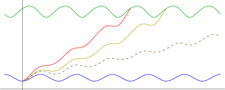
Figure 3: (a) The decreasing sequence $y_{n}$ has some limit $u$. (b) The $T$-periodic extension of $y$ is a new lower solution $\hat{\alpha}$.

(Phase 1d)                 $u$ is asymptotic to $x_{*}$ in the future.

To see this we consider the sequence of functions

$$u_{n}(t)=u(t+nT)\,,\hskip 56.9055ptt\in[0,T]\,,$$

which is uniformly bounded and pointwise increasing, and made of solutions of (1). We use again Proposition 2.6 to deduce that $\{u_{n}\}$ converges in the $\mathcal{C}^{2}[0,T]$ topology to some solution $u_{*}:[0,T]\to\mathbb{R}$ of (1). This solution must clearly be $T-$periodic and lie between $\alpha$ and $x_{\min}$. But $x_{\min}$ was minimal, meaning that $u_{*}=x_{\min}$. The result follows.

(Step 2) From a particular case to Theorem 3.1 in its full generality

The first step was devoted to show Theorem 3.1 for $u_{0}=\alpha(0)$ and assuming that $f$ is bounded between $\alpha$ and $\beta$. We successively remove these restrictions in the phases below:

(Phase 2a)   Let $f$ be bounded between $\alpha$ and $\beta$. Then, for any $u_{0}\in(\alpha(0),x_{\min}(0))$ there exists some lower solution $\hat{\alpha}$ of $(P)$ with $\alpha\leq\hat{\alpha}\leq x_{\min}$ and $\hat{\alpha}(0)=u_{0}$.

Fix some $u_{0}\in(\alpha(0),x_{\min}(0))$ and consider the Dirichlet problem

$$(D_{0})\equiv\begin{cases}-\ddot{y}=f(t,y,\dot{y})\,,\vspace{0.3cm}\\ y(0)=u_{0}=y(T)\,.\end{cases}$$

For this problem, $\alpha$ is a lower solution, while $x_{\min}$ is an upper solution. Thus, Proposition 2.4 states the existence of some solution $y:[0,T]\to\mathbb{R}$ of $(D_{0})$ which lies between $\alpha$ and $x_{\min}$.

We claim that $\dot{y}(0)>\dot{y}(T)$. Indeed, $\dot{y}(0)\not=\dot{y}(T)$ since otherwise the $T$-periodic extension $\hat{\alpha}$ of $y$ would be a solution of $(P)$, contradicting the minimality of $x_{\min}$. And if $\dot{y}(0)<\dot{y}(T)$ then $\hat{\alpha}$ would be an upper solution of $(P)$, implying the existence of some periodic solution between $\alpha$ and $\hat{\alpha}$ and contradicting again the minimality of $x_{\min}$. Thus, $\dot{y}(0)>\dot{y}(T)$ as claimed, and this means that $\hat{\alpha}$ is a lower solution of $(P)$, see Fig. 3(b).

Step 1 now implies that for every $u_{0}\in[\alpha(0),x_{\min}(0))$ there exists some solution $u_{r}:[0,+\infty)\to\mathbb{R}$ with $u_{r}(0)=u_{0}$ and $\alpha\leq u_{r}\leq x_{\min}$ on $[0,+\infty)$ which is asymptotic to $x_{\min}$ in the future. But all this work was done assuming $f$ is bounded between $\alpha$ and $\beta$. The last part of the proof is devoted to see that [N] is sufficient.

(Phase 2b)   From boundedness to the Nagumo condition.

Let now $f$ satisfy [N]. We use the Modification Lemma 2.7 and transform equation (1) accordingly. In view of the comments following the statement of the Lemma, the original and the modified equations have the same $T$-periodic solutions between $\alpha$ and $\beta$, and $x_{\min}$ continues to be the minimal one of them. The discussions before show that from each initial position $u_{0}\in[\alpha(0),x_{\min}(0))$ there starts some solution $u_{r}$ of our modified equation which lies between $\alpha$ and $\beta$ and is asymptotic to $x_{\min}$ in the future. But (iii) implies that they are indeed solutions of the original equation. The proof is complete.

∎

The result which closes this Section is a straightforward consequence of Theorem 3.1 and Proposition 2.3, and states the instability of the maximal and the minimal solutions produced by the periodic method of lower and upper solutions. Since the Nagumo condition [N] always holds in the conservative case, it may be seen as a generalization of Proposition 3.1 of [1]:

Corollary 3.2.

Assume [N] and uniqueness for initial value problems associated to (1). Assume also that $\alpha$ (resp. $\beta$) is not a solution of this equation. Then, $x_{\min}$ (resp. $x_{\max}$) is unstable, simultaneously in the past and in the future.

Proof.

Assume, for instance, that $\alpha$ is not a solution of (1). Then, Proposition 2.3 implies that $x_{\min}$, being a (non-strict) upper solution of $(P)$, verifies $\alpha(0)<x_{\min}(0)$. For every initial position $u_{0}\in\big{[}\alpha(0),x_{min}(0)\big{)}$, Theorem 3.1 states the existence of solutions

$$u_{l}:(-\infty,0]\to\mathbb{R},\hskip 56.9055ptu_{r}:[0,+\infty)\to\mathbb{R}\,,$$

which are asymptotic to $x_{\min}$ in the past and in the future respectively and verify (9). By uniqueness of initial value problems, $u_{l}<x_{min}$ and $u_{r}<x_{\min}$ on their respective domains. The result follows.

∎

4 The dynamics between two ordered solutions

In this Section $\alpha$ and $\beta$ are assumed to be solutions of the periodic problem $(P)$. In general this does not imply the existence of an unstable periodic solution between them, at least if by ‘instability’ we mean Lyapunov instability in the past and in the future. To check this assertion it suffices to consider the linear equation $-\ddot{u}=\dot{u}$. Observe that the periodic solutions are the constants, and all of them are unstable in the past, but stable in the future. We also notice that, at least for this example, the periodic solutions are always ordered and make up a continuous family.

Thus, we shall begin by setting ourselves under the opposite situations of $\alpha$ and $\beta$ being neighboring solutions of $(P)$; i.e., the only solutions $x$ of the periodic problem $(P)$ lying between $\alpha$ and $\beta$ are $x\equiv\alpha$ and $x\equiv\beta$. Neighboring solutions have previously been considered in the literature, including for instance in the Aubry-Mather theory, which uses variational arguments to show the existence of heteroclinics between neighboring global periodic minimals (see, e.g. Theorem 2.6.2 of [5]). The periodic problem $(P)$ which occupies us now may not have a variational structure, and assuming that it has one, the neighboring solutions $\alpha\leq\beta$ may not be minimal. Indeed, one easily finds examples of neighboring periodic solutions which are not connected by heteroclinics (think for instance on two consecutive equilibria of some autonomous equation $-\ddot{x}=V^{\prime}(x)$ lying at different potential levels). However, in this Section we shall see that one of the neighboring periodic solutions must be the limit of many asymptotic solutions, simultaneously in the past and in the future. Precisely:

Theorem 4.1.

Let $\alpha\leq\beta$ be neighboring solutions of $(P)$ and assume [N]. Then, either $x\equiv\alpha$ or $x\equiv\beta$ has the following property: for any initial position

$$u_{0}\in\Big{(}\alpha(0),\beta(0)\Big{)}\,,$$

there are solutions $u_{l}:(-\infty,0]\to\mathbb{R},\ \ u_{r}:[0,+\infty)\to\mathbb{R}$ of (1) with

$$u_{l}(0)=u_{0}=u_{r}(0)\,,\hskip 42.67912pt\alpha\leq u_{l}\leq\beta\ \text{ on }(-\infty,0]\,,\hskip 42.67912pt\alpha\leq u_{r}\leq\beta\ \text{ on }[0,+\infty)\,,$$

which are asymptotic to $x$ in the past and in the future respectively.

Proof.

We consider the set $\Sigma$ of solutions of (1) on the time interval $[0,T]$ which start and end at the same position (with possibly different derivative) and lie between $\alpha$ and $\beta$:

$$\Sigma:=\left\{u\in\mathcal{C}^{2}[0,T]\left|\begin{matrix}\ u\text{ solves }(\ref{eu0})\\ \vspace{-0.4cm}\\ \ u(0)=u(T)\\ \vspace{-0.4cm}\\ \ \alpha\leq u\leq\beta\text{ on }[0,T]\end{matrix}\right.\right\}\,.$$

Observe that this set contains the solutions $\alpha$ and $\beta$. Since they are assumed to be neighboring, other solutions $u\in\Sigma$ must verify $\dot{u}(0)\not=\dot{u}(T)$. We start our proof by showing that $\Sigma$, which is naturally endowed with $\mathcal{C}^{2}[0,T]$ topology, contains nontrivial connected subsets:

       Claim.

For each $0<\epsilon<\frac{1}{2}(\beta(0)-\alpha(0))$ there exists a continuum $\Sigma_{\epsilon}\subset\Sigma$ such that

$$\Big{\{}u(0):u\in\Sigma_{\epsilon}\Big{\}}=\Big{[}\alpha(0)+\epsilon,\beta(0)-\epsilon\Big{]}\,.$$

To show the Claim we first replace our equation $(\ref{eu0})$ with a modified one $(\tilde{1})$ as in Lemma 2.7. From (ii) and (iii) we see that

$$\Sigma=\left\{u\in\mathcal{C}^{2}[0,T]\left|\begin{matrix}u\text{ solves }(\tilde{1})\\ \vspace{-0.4cm}\\ u(0)=u(T)\in[\alpha(0),\beta(0)]\end{matrix}\right.\right\}\,.$$

By the comments following the proof of Lemma 2.7 in the Appendix we see that $(\tilde{1})$ may actually be rewritten in the form (16) for some globally bounded function $b$. Thus, for each $u_{0}\in[\alpha(0),\beta(0)]$, the solutions $u:[0,T]\to\mathbb{R}$ of (1) which lie between $\alpha$ and $\beta$ and verify $u(0)=u(T)=u_{0}$ may be written as the fixed points of a compact, bounded operator $\mathcal{F}_{u_{0}}$ on the space of $\mathcal{C}^{2}[0,T]$ functions vanishing at times $t=0,T$. The family $\big{\{}\mathcal{F}_{u_{0}}\big{\}}_{u_{0}}$ is uniformly bounded and depends continuously on $u_{0}$, and the result then follows from the usual continuation properties of the Leray-Schauder topological degree.

Having shown the Claim, let us complete the proof of the Theorem. We choose some sequence $\epsilon_{n}\searrow 0$ with $0<\epsilon_{n}<\big{(}\beta(0)-\alpha(0)\big{)}/2$ for every $n$. As observed before, the associated connected sets $\Sigma_{\epsilon_{n}}$ do not contain periodic solutions, and we deduce that for each $n$, either

1. All solutions $u\in\Sigma_{\epsilon_{n}}$ verify that $\dot{u}(0)>\dot{u}(T)$, or

2. All solutions $u\in\Sigma_{\epsilon_{n}}$ verify that $\dot{u}(0)<\dot{u}(T)$.

Observe that if $(p_{n}^{-})$ holds for some $n$ then the elements of $\Sigma_{\epsilon_{n}}$ when extended to the real line by periodicity become lower solutions of $(P)$. On the contrary, if $(p_{n}^{+})$ holds for some $n$ then the $T-$periodic extensions of the elements of $\Sigma_{\epsilon_{n}}$ make up upper solutions of $(P)$. We deduce that if there are infinitely many numbers $n$ for which $(p_{n}^{-})$ holds, then problem $(P)$ has some lower solution starting from each initial position $\alpha_{0}\in(\alpha(0),\beta(0))$; moreover,this lower solution lies between $\alpha$ and $\beta$. On the contrary, if there are infinitely many numbers $n$ for which $(p_{n}^{+})$ holds, then problem $(P)$ has some upper solution starting from each initial position $\beta_{0}\in(\alpha(0),\beta(0))$, and this upper solution lies between $\alpha$ and $\beta$. The result follows now from Theorem 3.1.

∎

An immediate consequence of Theorem 4.1 is given below:

Corollary 4.2.

Assume [N] and uniqueness of initial value problems. If $\alpha<\beta$ are neighboring solutions of the periodic problem $(P)$, one of them must be unstable, simultaneously in the past and in the future.

We observe that, even though the method of lower and upper solutions also works for first order equations, this result does not have an immediate extension there. For instance, $\alpha\equiv 0$ and $\beta\equiv 1$ are neighboring periodic solutions for $-\dot{u}=u(1-u)$, but $\alpha$ is stable in the future and $\beta$ is stable in the past. We owe this remark to R. Ortega.

At this moment we come back to the question formulated at the beginning of this Section: given ordered solutions $\alpha<\beta$ of the periodic (second-order) problem $(P)$, is it possible to find an unstable solution between them? We already know that the answer is ‘yes’ if $\alpha$ and $\beta$ are neighboring and ‘no’ in general. In the spirit of the counterexample mentioned before we shall say that the periodic problem $(P)$ is degenerate between $\alpha$ and $\beta$ if they may be linked by an increasing path of periodic solutions. Precisely, if there exists some $\mathcal{C}^{2,0}$ function

$$\Psi:\mathbb{R}\times[0,1]\to\mathbb{R}\,,\hskip 42.67912pt(t,s)\mapsto\Psi(t,s)\,,$$

such that

1. $\Psi(\cdot,0)=\alpha(\cdot),\ \ \Psi(\cdot,1)=\beta(\cdot)\,.$

2. $\Psi(\cdot,s)$ is a solution of the periodic problem $(P)$ for any $s\in[0,1]$.

3. $\Psi(t,s_{1})<\Psi(t,s_{2})$ if $s_{1}<s_{2}$.

This concept of degeneracy will be used to give a more precise answer to the question which opened this paragraph. We remark that the study of degeneracy is not new, for instance a related notion of degeneracy was considered in [7].

Proposition 4.3.

Assume uniqueness for initial value problems and [N]. If $\alpha<\beta$ are ordered solutions of $(P)$, one of the following hold:

1. There exists some solution $x$ of the periodic problem $(P)$ which is unstable in the past and in the future and lies between $\alpha$ and $\beta$.

2. $(P)$ is degenerate between $\alpha$ and $\beta$.

Proof.

We distinguish two possibilities; either $\alpha$ and $\beta$ enclose some ordered pair $\alpha\leq x_{1}<x_{2}\leq\beta$ of neighboring periodic solutions, or not. In the first case Corollary 4.2 immediately implies $(I)$; in the second case we are going to show $(II)$.

Thus, assume that between $\alpha$ and $\beta$ there are not pairs $x_{1}<x_{2}$ of neighboring periodic solutions. We consider the set $\mathcal{F}$ whose elements are totally ordered families $F\subset\mathcal{C}^{2}(\mathbb{R})$ of solutions of the periodic problem $(P)$ lying between $\alpha$ and $\beta$. Here, ‘totally ordered’ means that for any $F\in\mathcal{F}$ and $x_{1}\not=x_{2}\in F$ one has either $x_{1}<x_{2}$ or $x_{2}<x_{1}$.

The set $\mathcal{F}$ itself may be endowed with the partial order provided by inclusion. Observe that if $\mathcal{S}\subset\mathcal{F}$ is any totally ordered subset, then $F:=\bigcup_{S\in\mathcal{S}}S$ is an upper bound for $\mathcal{S}$. Consequently, by Zorn’s Lemma $\mathcal{F}$ must have some maximal element $F_{0}$.

       Claim.

The following hold:

1. Every monotone sequence $\{x_{n}\}_{n}\subset F_{0}$ converges in the $\mathcal{C}^{2}$ norm to some $x_{*}\in F_{0}$.

2. For each initial position $x_{0}\in[\alpha(0),\beta(0)]$ there exists an unique element $x\in F_{0}$ with $x(0)=x_{0}$.

We first show the Claim. In view of the Modification Lemma 2.7 it suffices to prove ($\mathfrak{F}_{1}$) assuming that $f$ is bounded between $\alpha$ and $\beta$. Now, the fact that every monotone sequence in $F_{0}$ converges in the $\mathcal{C}^{2}$ norm to some $T$-periodic solution follows immediately from Proposition 2.6, and the maximality of $F_{0}$ implies that this limit must belong to $F_{0}$.

To see ($\mathfrak{F}_{2}$) we first observe that, as a consequence of ($\mathfrak{F}_{1}$), the set

$$A:=\Big{\{}x(0):x\in F_{0}\Big{\}}$$

of initial positions of elements in $F_{0}$, must be closed. If $A$ were not the whole interval $[\alpha(0),\beta(0)]$ then it would mean the existence of pairs of neighboring solutions of $(P)$, which we are assuming that is not the case. Then, for each initial position $x_{0}\in[\alpha(0),\beta(0)]$ there exists some element $x\in F_{0}$ with $x(0)=x_{0}$, and since two such functions should intersect tangentially, ($\mathfrak{F}_{2}$) follows from the uniqueness of initial value problems associated to (1).

To conclude the proof of Proposition 4.3 we define

$$\Psi(t,s):=x_{s}(t)\,,\hskip 56.9055ptt\in\mathbb{R},\ s\in[0,1],$$

where $x_{s}$ is the only element of $F_{0}$ with $x_{s}(0)=(1-s)\alpha(0)+s\beta(0)$. Then $\Psi$ satisfies the three conditions (a),(b),(c) above and the result follows. ∎

When the equation is conservative, $-\ddot{u}=f(t,u)$, past and future Lyapunov stability become equivalent concepts. We close this Section with a result which is specific for the conservative case:

Corollary 4.4.

Assume that there is uniqueness for initial value problems associated to $-\ddot{u}=f(t,u)$, and that $\alpha<\beta$ are ordered $T$-periodic solutions. Then there is some unstable solution between them (it may be either $\alpha$, or $\beta$, or other).

Proof.

In view of Proposition 4.3, it suffices to consider the case in which the $T$-periodic problem associated to our equation is degenerate between $\alpha$ and $\beta$. Assume also that, for instance, $\alpha$ is stable and consider the solution $u$ verifying $u(0)=\alpha(0)$ and $\dot{u}(0)=\dot{\alpha}(0)+\epsilon$, where $\epsilon>0$ is small. On the maximal interval of time $\mathcal{I}$ where $u$ lies between $\alpha$ and $\beta$, it cannot cross tangentially a periodic solution, and then, the continuous function $s$ defined implicitly by

$$u(t)=\Psi\big{(}t,s(t)\big{)}\,,\hskip 56.9055ptt\in\mathcal{I}\,,$$

must satisfy $\dot{u}(t)>\Psi_{t}(t,s(t))$ for any time $t$ (here, $\Psi=\Psi(t,s)$ is given by the definition of degeneracy). One easily deduces from here that $s$ is strictly increasing on $\mathcal{I}$. On the other hand, the stability of $\alpha$ implies that $\mathcal{I}=[0,+\infty)$ and $s(t)$ converges to some small limit $0<\ell<1$ as $t\to+\infty$. It follows that the periodic solution $\Psi(\cdot,\ell)$ is unstable and concludes the proof. ∎

5 Appendix: Discussing the statements of Section 2

The last Section of this paper is devoted to sketch the proofs of some results which were presented in Section 2 and used subsequently.

Proof of Lemma 2.7.

It combines elements from the proofs of Theorem 5.4 of Chapter I of [2] on the one hand and Lemma 4.2 of [6] on the other. We start by letting

$$\tilde{f}(t,u,\dot{u}):=-u+\gamma(t,u)+f\big{(}t,\gamma(t,u),\delta(\dot{u})\big{)}\,,\hskip 42.67912pt(t,u,\dot{u})\in\mathbb{R}^{3}\,,$$ (12)

where

$$\gamma(t,u):=\begin{cases}\alpha(t)&\text{if }u\leq\alpha(t)\\ u&\text{if }\alpha(t)\leq u\leq\beta(t)\\ \beta(t)&\text{if }u\geq\beta(t)\end{cases}\,,\hskip 42.67912pt\delta(v):=\begin{cases}-K&\text{if }v\leq-K\\ v&\text{if }-K\leq v\leq K\\ K&\text{if }v\geq K\\ \end{cases}\,,$$

and the constant $K>0$ is chosen in such a way that

$$\int_{0}^{K}\frac{v}{\varphi(v)}\,dv>\beta(0)-\alpha(0)\,,\hskip 42.67912ptK>\max\Big{\{}\|\dot{\alpha}\|_{\infty},\|\dot{\beta}\|_{\infty}\Big{\}}\,.$$ (13)

Clearly, $\tilde{f}$ is continuous, $T$-periodic and bounded between $\alpha$ and $\beta$. Also (i) is immediate from the definition of $f$, while (iii) is a consequence of the Nagumo condition (choose $\epsilon>0$ small enough so that $\int_{\epsilon}^{K}v\,dv/\varphi(v)>\beta(0)-\alpha(0)$).

The proof of (ii) is less direct and will rely on three previous results which we describe next. The first and the third ones focus attention on the side limits

$$D_{l}h(t_{0}):=\underset{\begin{matrix}t\to t_{0}\\ t<t_{0}\end{matrix}}{\operatorname{ess\lim\ }}\dot{h}(t)\,,\hskip 56.9055ptD_{r}h(t_{0}):=\underset{\begin{matrix}t\to t_{0}\\ t>t_{0}\end{matrix}}{\operatorname{ess\lim\ }}\dot{h}(t)\,,$$

where $h$ is some Lipschitz-continuous function. The derivative $\dot{h}$ may exist only almost everywhere; thus, the limits above are ‘essential limits’, meaning that they must be considered after $\dot{h}$ is perhaps redefined on a zero-measure set. For arbitrary Lipschitz-continuous functions $h$ these limits do not always exist, but it cannot be the case when $h=\alpha$ is a lower solution of $(P)$:

1.  Regularity of lower solutions:  Let $\alpha$ be a lower solution of (P). Then, $D_{l}\alpha(t_{0})$ and $D_{r}\alpha(t_{0})$ exist for every $t_{0}\in\mathbb{R}$ and satisfy $D_{l}\alpha(t_{0})\leq D_{r}\alpha(t_{0})$.

Proof.

Let $\omega\in W^{2,\infty}_{loc}(\mathbb{R})$ be any second primitive of the function $\ddot{\omega}(t)=-f(t,\alpha(t),\dot{\alpha}(t))$, and let $h:=\omega-\alpha$. In this way, $h$ is locally Lipschitz-continuous and $-\ddot{h}\geq 0$ in the distributional sense. But positive distributions are positive, locally finite Borel measures (see e.g. Theorem 6.22 of [4]). Consequently, $\dot{h}$ is decreasing and has side limits at each point. The result follows. ∎

A second consequence of the fact that positive distributions are positive, locally finite Borel measures is a distributional version of the maximum principle in one dimension:

2. Maximum principle: Let $h:(a,b)\to\mathbb{R}$ be Lipschitz-continuous and verify

$$-\ddot{h}\geq 0\text{ on }(a,b)\,,$$

in the distributional sense. If $h$ attains a local minimum at some point $t_{0}\in(a,b)$ then it is constant.

Proof.

As before, $\dot{h}$ is a decreasing function. It implies the result.∎

The third result is an elementary observation which follows directly from our definition of the side limits $D_{l}h(t_{0})$ and $D_{r}h(t_{0})$. It gives information on these limits at any point $t_{0}$ where $h$ has a local minimum.

3. $D_{l}h$ and $D_{r}h$ at local minima: Let $h:(a,b)\to\mathbb{R}$ be Lipschitz-continuous and attain a local minimum at $t_{0}\in(a,b)$. Assume also that the limits $D_{l}h(t_{0})$ and $D_{r}h(t_{0})$ exist. Then $D_{l}h(t_{0})\leq 0\leq D_{r}h(t_{0}).$

Proof.

Integrating from $t_{0}$ to $t$ we see that, if $D_{l}h(t_{0})$ exists, then

$$\lim_{\begin{matrix}t\to t_{0}\\ t<t_{0}\end{matrix}}\frac{h(t)-h(t_{0})}{t-t_{0}}=D_{l}h(t_{0})\,,$$

i.e., the left-side derivative of $h$ at $t_{0}$ exists and has the same value. Similarly, if $D_{r}h(t_{0})$ exists at some point $t_{0}$, then the right-side derivative there also exists and coincides with $D_{r}h(t_{0})$. The result follows. ∎

We complete now the proof of statement (ii) of Lemma 2.7. We use a contradiction argument and assume, for instance, that $u:I\to\mathbb{R}$ is a solution of $(\tilde{1})$ such that $h:=u-\alpha$ attains a local minimum at some interior point $t_{0}\in I$ with $u(t_{0})<\alpha(t_{0})$. Since $u$ is a $\mathcal{C}^{1}$ function, result 1. above implies that the side limits $D_{l}h(t_{0}),\ D_{l}h(t_{0})$ exist and moreover $D_{l}h(t_{0})\geq D_{r}h(t_{0})$. But $t_{0}$ being a point where $h$ attains a local minimum, 3. gives that $D_{l}h(t_{0})=D_{r}h(t_{0})=0$, or what is the same,

$$\lim_{t\to t_{0}}\dot{\alpha}(t)=\dot{u}(t_{0})\,.$$ (14)

In particular, $|\dot{u}(t_{0})|\leq\|\dot{\alpha}\|_{\infty}$, and for any $t$ on some neighborhood of $t_{0}$ one has

$$u(t)<\alpha(t)\,,\hskip 56.9055pt|\dot{u}(t)|\leq K\,,$$

and then $-\ddot{u}(t)=-u(t)+\alpha(t)+f(t,\alpha(t),\dot{u}(t))$. Consequently, on this same neighborhood we have

$$-\ddot{h}(t)=-\ddot{u}(t)+\ddot{\alpha}(t)\geq-u(t)+\alpha(t)+f(t,\alpha(t),\dot{u}(t))-f(t,\alpha(t),\dot{\alpha}(t))\,,$$

and combining (14) with the continuity of $f$ we see that

$$-\ddot{h}(t)\geq\frac{1}{2}\,\big{(}-u(t_{0})+\alpha(t_{0})\big{)}>0$$ (15)

on some (possibly smaller) neighborhood of $t_{0}$. But $h$ attains a local minimum at $t_{0}$, so that in view of 2. above it should be constant on this neighborhood. Then, $-\ddot{h}\equiv 0$ there, contradicting (15). This contradiction proves the result.

∎

The proof of Lemma 2.7 actually gives some additional information which was not stated in Section 2. It implies that the nonlinearity $\tilde{f}$ may be chosen in such a way that $b(t,u,\dot{u}):=\tilde{f}(t,u,\dot{u})+u$ is globally bounded on $\mathbb{R}^{3}$. This allows us to rewrite $(\tilde{1})$ as

$$-\ddot{u}=-u+b(t,u,\dot{u})\,.$$ (16)

We are led to the existence result for the periodic method of lower and upper solutions.

Proof of Proposition 2.1.

Schauder’s Fixed-Point Theorem guarantees the existence of some $T$-periodic solution to (16). Since this equation is equivalent to $(\tilde{1})$, in view of the comments following the statement of Lemma 2.7 in Section 2 we see that this is a $T$-periodic solution of (1) lying between $\alpha$ and $\beta$. It implies the result. ∎

Proof of Proposition 2.6.

This result is very standard. Our assumptions imply that $\{u_{n}\}$ and $\{\ddot{u}_{n}\}$ are uniformly bounded sequences. Then, one easily checks that $\{\dot{u}_{n}\}$ must also be uniformly bounded and we conclude that $\{u_{n}\}$ and $\{\dot{u}_{n}\}$ are equicontinuous. Ascoli-Arzela’s lemma now implies that $\{u_{n}\}\to u$ in the $\mathcal{C}^{1}[0,T]$ topology. But since $u_{n}$ is a solution of (1) for each $n$ we deduce that $u$ solves the same equation and $\{u_{n}\}\to u$ in the $\mathcal{C}^{2}[0,T]$ topology. The result follows. ∎

Proof of Proposition 2.2.

Clearly we may focus attention on the part of the statement concerning $x_{\max}$. On the other hand, after possibly modifying $f$ as in Lemma 2.7 we may assume that it is bounded between $\alpha$ and $\beta$. We consider the set $\Gamma$ of periodic solutions which lie between them:

$$\Gamma:=\left\{x\in\mathcal{C}^{2}(\mathbb{R})\left|\begin{matrix}x\text{ solves }(P)\\ \vspace{-0.4cm}\\ \alpha\leq x\leq\beta\end{matrix}\right.\right\}$$

This set is naturally ordered by the pointwise order $\leq$. Using Proposition 2.6 we see that every totally ordered subset $A\subset\Gamma$ has an upper bound in $\Gamma$. Then, Zorn’s lemma implies the existence of some maximal element $x_{\max}$. It verifies

$$x\in\Gamma,\ \ x\geq x_{\max}\ \Rightarrow\ x\equiv x_{\max}\,.$$ (17)

Using a contradiction argument assume now that there exists $x_{*}\in\Gamma$ with

$$x_{*}(t_{0})>x_{\max}(t_{0})$$

for some $t_{0}\in\mathbb{R}$. Since $x_{*}\ngeq x_{\max}$, we may find times $t_{-}<t_{0}<t_{+}<t_{-}+T$ such that

$$x_{*}(t_{\pm})=x_{\max}(t_{\pm})\,,\hskip 56.9055ptx_{*}(t)>x_{\max}(t)\ \forall t\in[t_{-},t_{+}]\,.$$

We define $\alpha_{*}:\mathbb{R}\to\mathbb{R}$ by

$$\alpha_{*}(t):=\begin{cases}x_{*}(t)\text{ if }t\in[t_{-},t_{+}]\,,\\ x_{\max}(t)\text{ if }t\in(t_{+},t_{-}+T)\,,\end{cases}$$

and extended by periodicity. A simple integration-by-parts argument shows that $\alpha_{*}$ is a new lower solution of $(P)$. Since $\alpha_{*}\leq\beta$, Proposition 2.1 implies the existence of some $\tilde{x}\in\Gamma$ with $\tilde{x}\geq\alpha_{*}$, contradicting (17). This concludes the proof.

∎

The proofs of Propositions 2.4 and 2.5 use similar arguments to the proof of Proposition 2.2, and we shall not reproduce them here. We conclude the paper with the proof of Proposition 2.3, which follows along the lines of Lemma 2.4 of [3].

Proof of Proposition 2.3.

Using a contradiction argument, we assume that $\alpha\leq\beta$ is an ordered pair of lower and upper solutions of $(P)$ verifying

$$\alpha(t_{0})<\beta(t_{0})\,,\hskip 56.9055pt\alpha(t_{1})=\beta(t_{1})$$

for some $t_{0},t_{1}\in\mathbb{R}$. Using Lemma 2.7 it is not restrictive to assume that $f$ is bounded between $\alpha$ and $\beta$; moreover, the periodicity of $\alpha,\beta$ allows us to assume $t_{0}<t_{1}<t_{0}+T$. For any $y_{0}\in(\alpha(t_{0}),\beta(t_{0}))$ we consider the Dirichlet problem

$$(D_{y_{0}})\equiv\begin{cases}-\ddot{y}=f(t,y,\dot{y})\vspace{0.3cm}\\ y(t_{0})=y(t_{0}+T)=y_{0}\end{cases}\,.$$

Fix now points $y^{-}_{0}<y_{0}^{+}\in(\alpha(t_{0}),\beta(t_{0}))$. Since $\alpha$ and $\beta$ are lower and upper solutions for $(D_{y_{0}^{-}})$, Proposition 2.4 implies that this problem must have some solution $y^{-}$ lying between $\alpha$ and $\beta$. In turn, $y^{-}$ and $\beta$ are respectively lower and upper solutions for $(D_{y_{0}^{+}})$, which should have a solution $y^{+}$ lying between $y^{-}$ and $\beta$. Now, $y^{-}$ and $y^{+}$ coincide at $t=t_{1}$, and being ordered, they must be tangent there. This contradicts the uniqueness of initial value problems and concludes the proof. ∎

References

- [1] Dancer, E.N.; Ortega, R., The index of Lyapunov stable fixed points in two dimensions. J. Dynam. Differential Equations 6 (1994), no. 4, 631–637.
- [2] De Coster, C.; Habets, P., Two-point boundary value problems: lower and upper solutions. Mathematics in Science and Engineering, 205. Elsevier B. V., Amsterdam, 2006.
- [3] Jackson, L.K.; Schrader, K.W., Comparison theorems for nonlinear differential equations. J. Differential Equations 3 (1967) 248–255.
- [4] Lieb, E.H.; Loss, M., Analysis. Second edition. Graduate Studies in Mathematics, 14. American Mathematical Society, Providence, RI, 2001.
- [5] Moser, J. Selected Chapters in the Calculus of Variations. Lecture notes by Oliver Knill. Lectures in Mathematics ETH Zürich. Birkhäuser Verlag, Basel, 2003.
- [6] Ortega, R.; Robles-Pérez, A.M., A maximum principle for periodic solutions of the telegraph equation. J. Math. Anal. Appl. 221 (1998), no. 2, 625–651.
- [7] Ortega, R.; Tarallo, M., Degenerate equations of pendulum-type. Commun. Contemp. Math. 2 (2000), no. 2, 127–149.
- [8] Palis, J.; de Melo, W., Geometric theory of dynamical systems. An introduction. Springer-Verlag, New York-Berlin, 1982.
- [9] Ureña, A.J., All periodic minimizers are unstable. Arch. Math. (Basel) 91 (2008), no. 1, 63–75.
- [10] Ureña, A.J., Invariant manifolds around equilibria of Newtonian equations: Some pathological examples. J. Differential Equations, 249 (2010), no. 2, 366–391.