Selfconsistent descriptions of vector-mesons in hot matter revisited

Abstract

Technical concepts are presented that improve the selfconsistent treatment of vector-mesons in a hot and dense medium. First applications concern an interacting gas of pions and $\rho$ mesons. As an extension of earlier studies we thereby include RPA-type vertex corrections and further use dispersion relations in order to calculate the real part of the vector-meson selfenergy. An improved projection method preserves the four transversality of the vector-meson polarisation tensor throughout the selfconsistent calculations, thereby keeping the scheme void of kinematical singularities.

I Introduction

The study of the in-medium properties of hadrons has received considerable attention during the recent years. From chiral-symmetry considerations one expects strong changes in the spectral distribution of particles when approaching the phase transition form the hadronic phase into the quark-gluon plasma. Apart from interesting many-body effects like particle-hole excitations, scattering off particles from a heat bath or Landau-damping which are present at finite temperature and density such investigations also allow to gain insight into fundamental aspects of quantum chromodynamics (QCD), cf. e.g. Leupold:2009kz ; Rapp:2009yu ; Tserruya:2009zt . A special research focus has been on vector-mesons studied through their decay into electron–positron or muon–antimuon pairs, called dileptons. Void of complicated final-state interaction effects such electromagnetic signals directly observe the center of the reaction zone and therefore allow to get an unperturbed view on the medium modifications of the vector mesons. Here several collaborations studied vector-mesons and especially the $\rho$-meson in nucleus-nucleus Eberl:2005ks ; Matis:1994tg ; Wessels:2002ha ; Angelis:1998im ; Arnaldi:2006jq ; Adamova:2006nu and hadron-nucleus Naruki:2005kd ; Ozawa:2000iw collisions. In such experiments a significant enhancement in the dilepton rates was observed in the invariant pair-mass region of 300 to 600 MeV, compared to estimates from straight extrapolation of elementary processes. These observations triggered quite a variety of explanations, which range from a lowering of the $\rho$-meson mass to a significant increase of its damping width Asakawa:1992ht ; Herrmann:1993za ; Friman:1997tc ; Rapp:1997fs ; Peters:1997va ; Urban:1999im ; vanHees:2000bp ; Post:2000qi ; Cabrera:2000dx ; Riek:2004kx . Presently the high precision data of the NA60 collaboration Arnaldi:2006jq are best described assuming a strong broadening of the $\rho$-meson width in the medium vanHees:2007th ; Rapp:1999ej . This seems also to be compatible with results from hadron-nucleus collisions and photo-production experiments Ozawa:2000iw ; Clas:2007mga ; Wood:2008ee where also a broadening is favored and which could be explained by theoretical models Effenberger:1999ay ; Muhlich:2002tu ; Wood:2008ee ; Riek:2008ct ; Riek:2010gz . On the other hand the experimental results of Ref. Naruki:2005kd favor a mass shift of the $\rho$-meson with only little broadening.

So far most theoretical investigations were done on a perturbative level Urban:1999im ; Rapp:1999qu ; Rapp:1999us ; Rapp:1999ej ; Post:2003hu ; Post:2000qi ; Cabrera:2000dx . This allows to include large numbers of excitation modes contributing to the $\rho$-meson spectral function. selfconsistent treatments vanHees:2000bp ; Riek:2004kx ; Ruppert:2004yg ; Riek:2006vq ; RR-Eratum showed interesting new effects. However so far the model space in the latter studies was rather limited and mesonic systems where investigated only. In a previous work Riek:2004kx we already improved the situation by considering baryon effects on the pionic modes in the medium. Significant progress in the description of mesons and baryons on the vacuum level has been achieved by coupled channel approaches Penner:2002ma ; Penner:2002md ; Lutz:2001mi . In Lutz:2001mi this input was then used to draw conclusions about the in-medium behavior of vector-mesons. Here quite different effects as compared to the calculations of Post et. al. Post:2000qi were found due to the smaller coupling of the $\rho$-meson to the $N^{*}$(1520) resonance. Thus despite the recent success of several models in explaining the experimental data more theoretical investigations are needed in order to understand the dynamics in more detail.

In this work we will concentrate on some conceptual aspects which are important for the improvement of selfconsistent descriptions. The first concerns the treatment of vertex corrections initially studied already in Asakawa:1992ht ; Herrmann:1993za . For baryon systems , including self-consistency, their special role was shown in Refs. Lutz:2007bh ; Korpa:2008ut ; Riek:2008uw . Here we shall study their role in mesonic systems with the perspective to generalize the techniques to the coupled system of mesons and baryons Riek:2004kx ; Rapp:1999ej . As a second point we will address the issue of renormalization. So far in all selfconsistent treatments vanHees:2000bp ; Riek:2004kx ; Ruppert:2004yg ; Riek:2006vq ; RR-Eratum the real parts of the selfenergies were neglected. For renormalizable theories it was shown in vanHees:2001ik ; VanHees:2001pf ; vanHees:2002bv how a proper renormalization has to be performed. However since we are working within the framework of an effective field theory such a procedure is not applicable and we use dispersion relations or formfactors instead. For vector mesons one has to face the additional problem that due to the violation of certain Ward-identities also longitudinal modes will be propagated in selfconsistent approximation schemes. Several methods were proposed vanHees:2000bp ; Riek:2004kx ; Ruppert:2004yg ; Riek:2006vq ; RR-Eratum in order to cure this problem. They all have one or an other conceptual drawback Riek:2006vq especially linked to the appearance of kinematical singularities. Here we will show how the scheme introduced in vanHees:2000bp can be extended in order to deal with this problem.

The paper is organized as follows. In section II we provide an overview of the model and the approximation scheme used to develop our techniques within the selfconsistent framework. In section III we than go into more detail about the calculations, however, deferring more technical aspects to the appendices. The results will than be presented in section IV before concluding.

II The approximation scheme

The Lagrangian defining the interaction between the isospin triplet fields of pions and $\rho$-mesons, $\pi$ and $\rho$, is given by Urban:1998eg

$${\mathcal{L}}_{\pi\rho}^{vector}=\frac{1}{2}(\partial_{\mu}-ig\rho_{\mu}T^{1})\,\pi\cdot(\partial_{\mu}-ig\rho_{\mu}T^{1})\,\pi$$

$$\qquad\qquad\,-\frac{1}{2}m_{\pi}^{2}\pi\cdot\pi-\frac{1}{4}\rho_{\mu\nu}\rho^{\mu\nu}+\frac{1}{2}m_{\rho}^{2}\rho_{\mu}\rho^{\mu}$$ (1)

in vector representation (see e.g. Leupold:2006bp for a discussion of tensor representation). Here the isospin structure of the terms is not explicitly given. The vector meson couples to the pions through the fully anti-symmetrized tensor in isospin $T^{1}_{abc}=-i\epsilon_{abc}$ with isospin indices $a,b,c$. Thereby $\rho_{\mu\nu}=\partial_{\mu}\rho_{\nu}-\partial_{\nu}\rho_{\mu}$ denotes the vector-meson field strength tensor. The parameters $g=5.3$ and $m_{\rho}=773$ MeV are adjusted to the electromagnetic form factor of the pion and compare quite well to the values found in perturbative calculations. In order to avoid contributions from non-physical modes such as ghosts, the vector meson propagator will be treated in the unitary gauge limit, which pushes all non-physical modes to infinite masses. The expressions for the free pion and $\rho$-meson propagator then read

$$D^{0}(w)=\frac{1}{w^{2}-m_{\pi}^{2}+i\epsilon}\,,\quad G^{\,0}_{\mu\nu}(w)=\frac{g_{\mu\nu}-\frac{w_{\mu}\,w_{\nu}}{m_{\rho}^{2}}}{w^{2}-m_{\rho}^{2}+i\epsilon}.$$ (2)

The selfconsistent retarded propagators $D$ and $G_{\mu\nu}$ of pion and $\rho$-meson are given as solutions of the coupled set of Dyson equations

$$G_{\mu\nu}(w,u) = G^{\,0}_{\mu\nu}(w)+G^{\,0}_{\mu\alpha}(w)\,\Pi^{\alpha\beta}_{(\rho)}(w,u)\,G_{\beta\nu}(w,u)\,,$$

$$D(w,u) = D^{0}(w)+D^{0}(w)\,\Pi_{(\pi)}(w,u)\,D(w,u)\,.$$ (3)

In vanHees:2000bp ; Riek:2004kx ; Ruppert:2004yg only the lowest order selfenergy diagrams given by the interaction (1) were included. As an extension to this approach we will now also study a first set of vertex corrections which proved important in the description of baryons Asakawa:1992ht ; Herrmann:1993za ; Lutz:2007bh ; Korpa:2008ut ; Riek:2008uw . We start from the assumption that all soft modes of the system have to be resumed while the hard modes can be effectively treated as local point vertices. Then the key ingredient of our calculation is the correlation loop

$$\mathbf{\chi}^{\mu\nu} =\text{\parbox{62.59573pt}{\includegraphics[scale={0.5}]{Bubble}}}=\text{\parbox{62.59573pt}{\includegraphics[scale={0.5}]{BubblePRP}}}\,.$$ (4)

In a relativistic treatment it takes the form of a Lorentz polarization tensor. From the interaction Lagrangian (1) one can then construct the following resummed correlation functions

$$\Pi^{\mu\nu}= =\left[\chi\cdot\left(1-g\cdot\chi\right)^{-1}\right]^{\mu\nu}$$

$$\Gamma^{\mu\nu}= =g\cdot\Pi^{\mu\nu}\cdot g$$ (5)

$$\Gamma^{\mu}= =w^{\mu}+g\cdot\Pi^{\mu\nu}\,w_{\nu}\,,$$

which will provide standard random phase approximation RPA corrections to the selfenergies and vertices. Here $w_{\mu}$ denotes the external pion momentum. The differences between these three expressions result from the outer most vertices. For $\Pi$ there are two three-point vertices at the outer most positions, while $\Gamma^{\mu\nu}$ has two four-point vertices and $\Gamma^{\mu}$ one three and one four-point vertex.

For the resulting selfenergies we will omit contributions which are suppressed by phase-space constraints whenever two “simultaneous” $\rho$-meson lines implicitly occur in a diagram. The pion polarization function then becomes

$$\Pi_{\pi}=\text{\parbox{125.19147pt}{\includegraphics[scale={0.6}]{SPi1}}}\,$$

$$\qquad\left[+\,\text{\parbox{128.03673pt}{\vspace{-0.2cm}\includegraphics[scale={0.5}]{SPi2}}}\,\right.$$

$$\qquad\left.+\,\text{\parbox{122.3462pt}{\vspace{-0.7cm}\includegraphics[scale={0.6}]{SPi3}}}\right].\,$$

$$=-4\,w^{\mu}\,\Pi_{\mu\nu}\,w^{\nu}+\delta m_{\pi}+w^{2}\,\delta,$$ (6)

The first diagram gives the main contribution. It corrects the $\pi\rho$-loop in the pion selfenergy by short-range correlations. The two diagrams in brackets will be omitted since they are suppressed by phase-space constraints. The renormalization terms $\delta m_{\pi}$ and $\delta$ in (6) will be adjusted in vacuum to guarantee that the pion has its pole at $m^{2}=(139\text{ MeV})^{2}$ with residuum 1. The polarization tensor of the $\rho$-meson is then given by

$$\Pi_{\rho} = \Pi_{(\rho,1)}+\Pi_{(\rho,2)}\qquad\text{with}$$

$$-i\Pi_{(\rho,1)} = \text{\parbox{76.82204pt}{\vspace{-0.1cm}\includegraphics[scale={0.36}]{SRho1}}}\,+\text{\parbox{76.82204pt}{\includegraphics[scale={0.36}]{SRho3}}}+\dots$$

$$-i\Pi_{(\rho,2)} = \text{\parbox{85.35782pt}{{\vspace{+0.5cm} \includegraphics[scale={0.4}]{SRho4}}}}\,,$$ (7)

where zero or at most one correlation bubble $\Gamma^{\mu}$ can be attached to the external vertices of $\Pi_{(\rho,1)}$, the latter due to the $\pi\pi\rho\rho$ coupling of the Lagrangian (1). Again phase-space suppressed terms can be dropped. In the end we arrive at a set of coupled Dyson equations for the determination of the full retarded propagators in terms of the retarded selfenergies or polarization tensors and the free propagators. Details about the calculation will be given in the next section. Readers only interested in the results could skip the next section and directly jump to the result section.

III Details of the calculation

III.1 Pion selfenergy and polarization loops

It is advantageous to decompose the central correlation loop (4) into its Lorentz tensor components (see e.g. Lutz:2002qy )

$$\chi_{\mu\nu}(w,u)= \sum_{i,j=1}^{2}\,\chi_{ij}(w,u)\,L_{\mu\nu}^{(ij)}(w,u)$$ (8)

$$+\chi_{\,T}(w,u)\,T_{\mu\nu}(w,u)\,.$$

Here $T_{\mu\nu}$ and $L_{\mu\nu}^{(22)}$ are the special projectors on the two spatially transverse and the spatially longitudinal modes. The other three $L_{\mu\nu}^{(ij)}$ complete the tensor algebra. Furthermore $w$ and $u$ denote the external four momentum and the four velocity of the equilibrated matter, respectively (in the c.m. frame of the matter $u=(1,\vec{0}\,)$). This decomposition will simplify the solution of the Dyson equation (3) as it provides a decoupling between the longitudinal and transversal sectors Lutz:2002qy . The derivation of the explicit expressions for the components $\chi_{ij}$ and $\chi_{\,T}$ is relegated to Appendix A. They simply follow from contractions of the tensor $\chi_{\mu\nu}(w,u)$ with the projectors. The decompositions (8) also easily allow to include the vertex corrections. We first define the loop matrices $\chi^{(L)}$ and $\chi^{(T)}$

$$\chi^{(L)}=\left(\begin{array}[]{ll}\chi_{11}&\chi_{12}\\ \chi_{21}&\chi_{22}\end{array}\right)\,\,,\quad\!\chi^{(T)}=\left(\begin{array}[]{l}\chi_{T}\end{array}\right).$$ (12)

The quantity $\Pi_{\mu\nu}(w,u)$, which sums up all correlations, then results to

$$\Pi_{\mu\nu}(w,u)= \sum_{i,j=1}^{2}\,\Pi_{(ij)}(w,u)\,L_{\mu\nu}^{(ij)}(w,u)$$ (13)

$$+\Pi_{(T)}(w,u)T_{\mu\nu}(w,u)$$

with coefficient functions $\Pi_{ij}$ and $\Pi_{T}$ defined as

$$\Pi_{(ij)}=\Big{[}\Big{(}\hbox{$1\hskip-1.2pt\vrule depth=0.0pt,height=6.88889pt,width=0.7pt\vrule depth=0.0pt,height=0.3pt,width=1.19995pt$}-\chi^{(L)}\,\Big{)}^{-1}\chi^{(L)}\Big{]}_{ij}$$

$$\Pi_{(T)}=\Big{[}\Big{(}\hbox{$1\hskip-1.2pt\vrule depth=0.0pt,height=6.88889pt,width=0.7pt\vrule depth=0.0pt,height=0.3pt,width=1.19995pt$}-\chi^{(T)}\,\Big{)}^{-1}\chi^{(T)}\Big{]}\,.$$ (14)

Due to the derivative structure of the interactions (1) and the structure of the four particle interactions the $\Gamma$-bubble insertions (II) and (7) simply lead to a replacement of the bare pion momentum $w^{\mu}$ at the vertex by a dressed one

$$w_{\nu}\;\rightarrow\;\Gamma_{\nu}(w,u) =w^{\nu}+w^{\mu}\,\Gamma_{\mu\nu}(w,u)$$

$$=w_{\nu}\,\Gamma_{1}(w,u)+u_{\nu}\,\Gamma_{2}(w,u)\,,$$

with contributions proportional $w^{\mu}$ and $u^{\mu}$ given by the vertex functions $\Gamma_{i}$. These vertex functions are obtained by contracting the full correlation sum $\Pi_{\mu\nu}(w,u)$ over $w^{\mu}$ because one vertex directly couples to the pion while the other one stems from the four point coupling. The two vertex functions $\Gamma_{1}(q,u)$ and $\Gamma_{2}(q,u)$ are explicitly given by

$$\Gamma_{1} =1+2\,\Big{[}\Big{(}\hbox{$1\hskip-1.2pt\vrule depth=0.0pt,height=6.88889pt,width=0.7pt\vrule depth=0.0pt,height=0.3pt,width=1.19995pt$}-g\,\chi^{(L)}\Big{)}^{-1}g\,\chi^{(L)}\Big{]}_{11}$$

$$+\frac{2\,(u\cdot w)}{\sqrt{w^{2}-(u\cdot w)^{2}}}\Big{[}\Big{(}\hbox{$1\hskip-1.2pt\vrule depth=0.0pt,height=6.88889pt,width=0.7pt\vrule depth=0.0pt,height=0.3pt,width=1.19995pt$}-g\,\chi^{(L)}\Big{)}^{-1}g\,\chi^{(L)}\Big{]}_{12}$$

$$+\delta\Gamma$$

$$\Gamma_{2} =\frac{-2\,w^{2}}{\sqrt{w^{2}-(u\cdot w)^{2}}}\,\Big{[}\Big{(}\hbox{$1\hskip-1.2pt\vrule depth=0.0pt,height=6.88889pt,width=0.7pt\vrule depth=0.0pt,height=0.3pt,width=1.19995pt$}-g\,\chi^{(L)}\Big{)}^{-1}g\,\chi^{(L)}\Big{]}_{12}$$

in terms of the loop functions (8). We further introduced a finite renormalization $\delta\Gamma$ in order to impose the condition $\Gamma_{1}(w^{2}=m_{\pi}^{2})=1$ in vacuum. There are two important technical issues to be emphasized here. First, the application of the longitudinal and transverse projectors in (8) implies that the loop functions have to satisfy specific constraints. They follow from the observation that the polarization tensor $\chi_{\mu\nu}(w,u)$ is regular. In particular at $w^{2}=0$ and at $w^{2}=(w\cdot u)^{2}$ it must hold that

$$\chi_{22}(w,u)=\chi_{11}(w,u)-i\,\chi_{12}(w,u)-i\,\chi_{21}(w,u)$$

$$\qquad\qquad\qquad+{\mathcal{O}}\left(w^{2}\right)\,,$$

$$\chi_{22}(w,u)=\chi_{T}(w,u)+{\mathcal{O}}\left((w\cdot u)^{2}-w^{2}\right)\,.$$

(17)

These conditions turn out to be important when specifying the real parts of the loop functions (see Appendix A). Furthermore a finite renormalization should be performed such that it suppresses the formation of ghosts in the pion selfenergy Korpa:2008ut . The construction of the latter has also to comply with the constraints (17).

III.2 Vector meson selfenergies

Concerning the vector-meson polarization tensor special care has to be taken about two issues: Its four transversality and the determination of its regularized real part. Let us start with the four transversality. A simple analysis of the Lorentz tensor decomposition of $\Pi_{\rho}$ (7) into the projector basis, similar as for (8) or (13), will directly show that only in the perturbative case no four longitudinal modes arise. The Dyson resummation (3) will lead to non vanishing four-longitudinal components, i.e. $\Pi^{(11)}_{(\rho)}\neq 0$ and $\Pi^{(12)}_{(\rho)}=\Pi^{(12)}_{(\rho)}\neq 0$. This problem originates from the violation of Ward-identities in the selfconsistent treatment. Several schemes were proposed in literature to cure this problem vanHees:2000bp ; Riek:2004kx ; Ruppert:2004yg ; Riek:2006vq ; RR-Eratum All schemes rely on some projection procedure

$$\Pi^{(ij)}_{(\rho)},\,\Pi^{(T)}_{(\rho)}\,\longrightarrow\,\Pi^{(22)}_{(\rho,P)},\,\Pi^{(T)}_{(\rho,P)}$$ (18)

where from the selfconsistently calculated $\Pi_{(\rho)}$ with its coefficients on the left a fully four-transversal structure of $\Pi_{(\rho,P)}$ is determined. However, as pointed out in Riek:2006vq all schemes used so far violate some of the constraints (17) and therefore suffer from the occurrence of kinematical singularities. As shown in Riek:2006vq such singularities have a substantial influence on the calculation. Here we will follow the scheme introduced by van Hees and Knoll vanHees:2000bp and show how it could be modified to avoid this problem. This scheme respects particular dynamical properties of the polarization tensor. It exploits the fact that the spatial components of the polarization tensor $\Pi^{ik}_{(\rho)}$ have a finite relaxation time and are of no particular harm. Thus they can be kept $\Pi_{(\rho,P)}^{ik}=\Pi_{(\rho)}^{ik}$. The time-components, however, involve an infinite relaxation time, since they carry the information about the conservation laws. Such components can never reliably be calculated at finite loop order. These time components can however be constructed solely from the spatial components such that the full tensor becomes four-transversal. Thus, the scalar functions $\Pi^{(22)}_{(\rho,P)}$ and $\Pi^{(T)}_{(\rho,P)}$ of the three physical modes, the spatially longitudinal and transverse ones, are calculated solely from the spatial parts of the polarization tensors using the following spatial traces

$$\Pi_{1}=\! \frac{w_{i}w_{k}}{\vec{w}^{\,2}}\Pi^{ik}_{(\rho)};\qquad\quad 3\Pi_{3} \!=-g_{ik}\Pi^{ik}_{(\rho)}$$ (19)

$$\Pi_{(\rho,\,P)}^{(22)}=\! \frac{w^{2}}{(u\cdot w)^{2}}\cdot\Pi_{1};\quad\;\Pi_{(\rho,\,P)}^{(T)} \!=\frac{1}{2}\left(3\Pi_{3}-\Pi_{1}\right).\quad$$ (20)

Therefore this scheme has a physically sound background. However unless $\Pi_{1}$ vanishes quadratically towards zero energy $w^{0}=(u\cdot w)$, which generally will not be the case, a singularity occurs Riek:2006vq . Placed in the space-like region the corresponding spurious zero energy mode does not directly affect physical observables such as dilepton spectra. It will however influence the selfconsistent dynamics, if the coupling of vector-mesons back onto other particles in the system is considered.

The advantage of this scheme is that it is free of singularities in the entire time-like region. It therefore opens the perspective to construct a singularity free tensor by some infrared cut-off procedure solely applied to the spatial longitudinal component $\Pi_{(\rho,\,P)}^{(22)}$ in the space-like region close to vanishing energy. To do so we rewrite the relation for the longitudinal projector (20) as

$$\Pi_{(\rho,\,P)}^{(22)}= \Pi^{(22)}_{(\rho)}-\frac{(u\cdot w)^{2}-w^{2}}{(u\cdot w)^{2}}\,\Pi^{(11)}_{(\rho)}$$ (21)

$$+2i\,\frac{\sqrt{(u\cdot w)^{2}-w^{2}}}{(u\cdot w)}\,\Pi^{(12)}_{(\rho)},$$

where we used $\Pi^{(21)}_{(\rho)}=\Pi^{(12)}_{(\rho)}$. In this formulation we directly see that (17) is perfectly reproduced on the light cone so the selfenergy is free of singularities there. The same is true at vanishing spatial momentum. The singularities stem from the factors in front of $\Pi^{(11)}_{(\rho)}$ and $\Pi^{(12)}_{(\rho)}$ at $(u\cdot w)=0$. Thus one can attempt to construct the $\Pi^{(22)}_{(\rho,\,P)}$ and $\Pi^{(T)}_{(\rho,\,P)}$ coefficients as

$$\Pi^{(T)}_{(\rho,\,P)}=\Pi_{(\rho)}^{(T)}$$ (22)

$$\Pi^{(22)}_{(\rho,\,P)}=\Pi^{(22)}_{(\rho)}-\lambda(w,u)\,\Pi^{(11)}_{(\rho)}-2i\,\sqrt{\lambda(w,u)}\,\Pi^{(12)}_{(\rho)}$$

with a coefficient function $\lambda(w,u)$, which has to fulfill

$$\lambda(w^{2}=0,u)=1$$ (23)

and should stay finite towards $(u\cdot w)=0$. A possible choice that provides a smooth transition to the form (21), which we would like to keep due to its physical motivation is given by

$$\lambda(w,u)\! = \!\!\left\{\!\!\begin{array}[]{ll}\frac{(u\cdot w)^{2}-w^{2}+\Lambda^{2}}{2((u\cdot w)^{2}+\Lambda^{2})}+\frac{(u\cdot w)^{2}-w^{2}}{2(u\cdot w)^{2}-w^{2}}&\mbox{for }w^{2}<0\\[5.69054pt] \frac{(u\cdot w)^{2}-w^{2}}{(u\cdot w)^{2}}&\mbox{for }w^{2}>0.\end{array}\right.$$ (26)

Here the parameter $\Lambda$ regularizes the infrared singularity and controls the strength in the far space like region. Later variations of $\Lambda$ can then be used to control the uncertainty introduced by the cut-off.

We now now turn to the determination of the real parts. Since the imaginary parts of the loops do not drop to zero for large energies renormalization is required which we introduce using subtracted dispersion relations. Thereby one has to keep in mind that along with the imaginary parts also the real parts have to be free from kinematical singularities and thus have to fulfil (17).

At the vacuum level it suffices to consider the following subtracted dispersion relation

$$\Pi^{(22/T)}_{(\rho,\,P)}(w)=\frac{1}{\pi}\,\int d\bar{w}_{0}\,\frac{w^{4}}{\bar{w}^{4}}\frac{\Im\,\Pi_{(\rho,\,P)}^{(22/T)}(\bar{w})}{w_{0}-\bar{w}_{0}+i\epsilon}$$ (27)

with $w=(w_{0},\vec{w}\,)$ and $\bar{w}=(\bar{w}_{0},\vec{w}\,)$. It automatically guarantees that the polarization tensor and its derivative vanish on the light cone so that the kinematical constraints (17) are naturally fulfilled. This technically preferred renormalization guarantees a massless photon with pole residuum 1 within the vector dominance picture. However, once medium effects come into play and all thresholds become effectively removed, the imaginary parts do no longer vanish on the light cone. One method to extend the prescription to the in-medium situation, is to first convert the description to a singularity free basis, then perform the dispersion integrals which are then free of any constraints and subsequently reconvert back Phd-Riek to the tensor decomposition. After combining all this together with the vacuum prescription we obtain

$$\Pi^{(T)}_{(\rho,\,P)}(w,u)=\Pi^{(T)}_{(\rho,vac)}(w,u)$$

$$+\int\frac{(u\cdot w)^{2}}{(u\cdot\bar{w})^{2}}\frac{\Im\,\Pi^{(T)}_{(\rho,\,P)}(\bar{w},u)-\Im\,\Pi^{(T)}_{(\rho,vac)}(\bar{w},u)}{\bar{w}_{0}-w_{0}+i\epsilon}\,d\bar{w}_{0}$$

$$\Pi^{(22)}_{(\rho,\,P)}(w,u)=\Pi^{(22)}_{(\rho,vac)}(w,u)$$

$$+\int\frac{w^{2}}{{\bar{w}}^{2}}\frac{\Im\,\Pi^{(22)}_{(\rho,\,P)}(\bar{w},u)-\Im\,\Pi_{(\rho,vac)}^{(22)}(\bar{w},u)}{\bar{w}_{0}-w_{0}+i\epsilon}\,d\bar{w}_{0}\,.$$

(28)

Here it is understood that the vacuum terms $\Pi^{(T)}_{(\rho,vac)}$ and $\Pi^{(22)}_{(\rho,vac)}$ already contain the projection to restore four transversality. The factor $w^{2}$ in the spatially longitudinal term is essential to cancel the $1/w^{2}$ singularity arising from the projector. The prescription then automatically guaranties that the three longitudinal and three transversal parts become degenerate for zero spatial momentum.

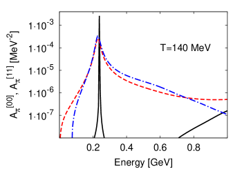
Figure 1: Pion spectral function $A^{[00]}_{\pi}$ (dashed line) and the effective spectral function $A_{\pi}^{[11]}$ (dashed dotted line) at $T=140$ MeV compared to the vacuum spectral function (full line) for a momentum of 200 MeV.

Now we comment about the inclusion of vertex corrections. They can be included along the lines of Refs. Korpa:2008ut ; Phd-Riek by introducing effective spectral functions which include the vertex structure (III.1)

$$A_{\pi}^{[ij]}(q,u)=-2\,\Im\left[\frac{\Gamma_{i}(q,u)\,\Gamma_{j}(q,u)}{q^{2}-m_{\pi}^{2}-\Pi_{\pi}(q,u)}\right]\,.$$ (29)

We further define $\Gamma_{0}(q)=1$ which allows us to write the normal pion spectral function as $A_{\pi}^{[00]}(q,u)$. Collecting then the vertex tensors $\Gamma_{i}$ into the pion spectral functions as defined in (29) the expressions for the imaginary parts of the selfenergies (7) can straight forwardly be evaluated. The results can be found in Appendix A.1. From these the complete polarization tensors can be calculated using (III.2) and (28).

IV Results

As the main focus of our work is on the conceptual developments, we keep this section rather brief, concentrating on the most relevant results only. First we analyze the influence of the cut-off $\Lambda$ introduced through the projection scheme (26). We found only a small sensitivity on the choice of the interpolation and therefore use a value of $\Lambda=200$ MeV in the following. This is good news because it shows that as soon as these space-like modes are treated properly their influence is rather small and the treatment with some a priori unknown infrared cut-off does not introduce a large uncertainty in the calculations.

From analytic estimates and earlier calculations Riek:2004kx we expect no dramatic changes of the spectral distribution of the $\rho$-meson. The most interesting point will be what influence the vertex corrections have on the result and to what extend the pion gets modified through selfconsistency.

In Fig. 1 the resulting pion spectral function is presented for zero and 140 MeV temperature. As compared to the vacuum case we observe that in the medium the gap between the on-shell pole and the $\rho\pi$-continuum becomes filled and that the on-shell peak gets broadened. In addition low energy components arise due to scattering off thermal pions. The effect of the vertex correction can be seen when comparing $A^{[00]}_{\pi}$ with $A_{\pi}^{[11]}$. Since $\Gamma_{1}$ is complex, also the real part of the pion propagator contributes to $A_{\pi}^{[11]}$. Since far away from the pole the real part is much larger than the imaginary part and changes sign at the pion pole, one obtains a destructive interference at low energies and some enhancement in the region between the on-shell pole and the continuum. This shift in pion strength leads to a reduced broadening of the $\rho$-meson as compared to the case without vertex correction because the phase space for the decay becomes reduced. However the influence of the vertex is much smaller then in the case of baryonic excitations Korpa:2008ut as could already be expected from the rather high threshold of the $\rho\pi$-loop as compared to the pion mass. Effects arising from the other components of the effective spectral function are zero in vacuum and stay negligible in the medium so that we do not discuss them here.

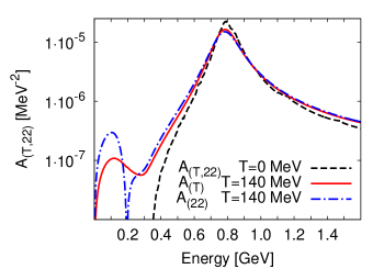
Figure 2: Spectral functions of the $\rho$-meson at $T=140$ MeV compared to the vacuum spectral function. The momentum is 200 MeV. For the spatially longitudinal spectral function $A_{(22)}$ the values are negative below the light cone, i.e. below 200 MeV.

The $\rho$-meson spectral function shows only minor changes. Noteworthy is that the partial width resulting from the decay into a pion pair becomes reduced at higher temperatures (see Fig. 2 and 3). This is caused by the asymmetry of the pion spectral function around the pole mass which receives a larger strength on the high mass side due to the $\rho\pi$ cut and therefore kinematically disfavors the decay of the $\rho$-meson. The resulting net effect between this reduction and the thermal enhancement turns out to be quite small such that the actual enhancement of the $\rho$-meson width mainly stems from the new decay mode into $\rho\pi\pi$ channel (cf. $\Pi_{\rho,2}$ in (7)) which has a lower threshold in dense matter once all particles attain broad spectral distributions. However even with the additional scattering and decay possibilities into the $\rho\pi\pi$ channel the width is only marginally increased by 35 MeV at 140 MeV temperature (see Fig. 3). In all cases the momentum dependence proved to be small.

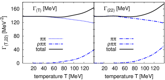
Figure 3: Spatially transverse and longitudinal damping widths of the $\rho$-meson versus temperature divided into the two dominant partial channels.

V Conclusions

In this work we developed some technical concepts for the in-medium treatment of vector mesons in a selfconsistent framework. Therefore we studied the influence of the presence of hot matter on the spectral properties of the $\rho$ meson. The aim was to include short-range correlations of the Migdal type in order to consistently sum up all soft modes of the system. These short-range correlations which are normally used to describe the interactions of the pion with nucleon and $\Delta$-isobar were now also applied to the vector-mesons in a selfconsistent framework. Special emphasis was put on the determination of the real-parts of all selfenergies and the proper avoiding of kinematical singularities in the selfconsistent scheme. The treatment of vector-mesons within the current model setup requires great care due to the fact that the polarization tensors have to be kept four transversal in order to avoid the propagation of unphysical degrees of freedom.

In the purely mesonic system containing pions and $\rho$ mesons no large medium effects were obtained, neither at high temperatures nor due to the here considered correlations and vertex corrections. This complies with earlier studies Rapp:1999ej ; Peters:1997va ; Post:2000qi ; Herrmann:1993za ; Friman:1997tc , where it was found that the dominating in-medium effects on the light vector-mesons result from the direct interaction with baryons. We only observe a moderate broadening of about 30 MeV for both vector-mesons even at 140 MeV temperature. However, compared to the perturbative treatment the selfconsistent scheme suggest a further source of the broadening, namely the $\rho\pi\pi$ decay. Of course this picture will be greatly influenced by the presence of low energy particle-hole excitations in the pion channel possibly leading to different conclusions in a more complete model. The influence of the vertex corrections and short range correlations turned out to be quite small compared to the over-all size of the selfenergies. On the other hand interesting new effects have been found which are necessary to understand the microscopic interactions in more detail. The influence of both vertex corrections and selfconsistency is expected to become important, once the scheme is extended to include the direct coupling to baryons. Then new low energy resonance-hole excitations come into play Korpa:2008ut . Using the formalism developed in this work and in Korpa:2008ut such extensions can be addressed in the future.

Acknowledgments

The authors acknowledge fruitful discussions with M.F.M. Lutz, B. Friman, R. Rapp, S. Leupold, D. Rischke, J. Ruppert and D. Voskresensky at various stages of this work. FR was supported by U.S. NSF grants PHY-0449489 (CAREER) and PHY-0969394.

Appendix A $\pi\rho$ loop tensor coefficients

The correlation loop (4) is defined as:

$$\mathbf{\chi}^{\mu\nu} =8g^{2}\int\frac{d^{4}l}{2(2\pi)^{4}}G_{\mu\nu}(l,u)\,D(l-w,u)\,.$$ (30)

The $\pi\rho$ loop contains an isospin factor of two due to isospin symmetry. In contrast to the dispersion relation strategy employed for the vector-meson, we here use a formfactor

$$F(q^{2})=\left(\exp\left(\frac{w^{2}-\lambda^{2}}{\lambda^{2}}\right)\right)^{2}\theta(w^{2}-\lambda^{2})+\theta(\lambda^{2}-w^{2})$$

with $\lambda=1250$ MeV, since some hard scale could be chosen without problems. The imaginary parts of the $\rho\pi$ loop functions $\chi_{ij}$ of Eq. (8) are then given by

$$\Im\chi_{ij}(w,u)=2g\int\frac{d^{4}l}{(2\pi)^{4}}\,(H^{[ij,22]}\,A^{\rho}_{22}(l,u)+H^{[ij,T]}\,A^{\rho}_{T}(l,u))\,A^{[00]}_{\pi}(l-w,u)\,(n_{B}(l\cdot u)-n_{B}((l-w)\cdot u))\,F(w^{2})\,,$$

$$\Im\chi_{T}(w,u)=2g\int\frac{d^{4}l}{(2\pi)^{4}}\,(H^{[T,22]}\,A^{\rho}_{22}(l,u)+H^{[T,T]}\,A^{\rho}_{T}(l,u))\,A^{[00]}_{\pi}(l-w,u)\,(n_{B}(l\cdot u)-n_{B}((l-w)\cdot u))\,F(w^{2})\,,$$

in terms of coefficients $H^{[11,22]}$ and $H^{[11,T]}$ specified at the end of this section (33) and the $\rho$-meson spectral function $A^{\rho}$ which has also been decomposed using the projector algebra. In addition we have to take care about the kinematical constraints. This can be realized along the lines presented in Korpa:2008ut for baryonic loops by choosing a different representation

$$\chi_{11}(\omega,\vec{q}\,)=\frac{1}{q^{2}}\,\chi_{1}(\omega,\vec{q}\,)\,,\qquad\chi_{12}(\omega,\vec{q}\,)=\frac{1}{\sqrt{q^{2}-(q\cdot u)^{2}}}\Bigg{(}\frac{q\cdot u}{q^{2}}\,\chi_{1}(\omega,\vec{q}\,)-\chi_{2}(\omega,\vec{q}\,)\Bigg{)}\,,$$ (32)

$$\chi_{22}(\omega,\vec{q}\,)=\frac{q\cdot u}{q^{2}-(q\cdot u)^{2}}\,\Bigg{(}\frac{q^{2}}{q\cdot u}\,\chi_{3}(\omega,\vec{q}\,)-2\,\chi_{2}(\omega,\vec{q}\,)\Bigg{)}\,,\quad\chi_{T}(\omega,\vec{q}\,)=\frac{1}{2}\,\left(\chi_{4}(\omega,\vec{q}\,)-\chi_{11}(\omega,\vec{q}\,)-\chi_{22}(\omega,\vec{q}\,)\right)\,.$$

The new functions $\chi_{i}$ can now be obtained, using the kernels defined in (33),

$$\chi_{i}(\omega,\vec{q}\,)=\Bigg{[}\delta_{i4}\,\chi_{3}(0,\vec{q}\,)-2g\int\frac{d^{4}l}{(2\pi)^{4}}\int_{-\infty}^{+\infty}\frac{d\bar{\omega}}{\pi}\,\left(\frac{q^{2}}{\bar{q}^{2}}\right)^{n_{i}}\,\frac{(H^{[i,22]}\,A^{\rho}_{22}(l,u)+H^{[i,T]}\,A^{\rho}_{T}(l,u))}{\bar{\omega}-\omega-i\,\epsilon}$$

$$\qquad\qquad\qquad\times A^{[00]}_{\pi}(l-w,u)\,(n_{B}(l\cdot u)-n_{B}((l-w)\cdot u))\,F(w^{2})\Bigg{]}\quad\;+(q_{\mu}\to-q_{\mu})\,,$$

for $i=1,3,4$ with $n_{1,4}=2$, $n_{2}=1$ and $q^{2}=\omega^{2}-\vec{q}^{\,2}$, $\bar{q}^{2}=\bar{\omega}^{2}-\vec{q}^{\,2}$. While for $n=2$ we have

$$\chi_{i}(\omega,\vec{q}\,)=\Bigg{[}\delta_{i4}\,\chi_{3}(0,\vec{q}\,)-2g\int\frac{d^{4}l}{(2\pi)^{4}}\int_{-\infty}^{+\infty}\frac{d\bar{\omega}}{\pi}\,\left(\frac{\omega}{\bar{\omega}}\right)\,\frac{(H^{[i,22]}\,A^{\rho}_{22}(l,u)+H^{[i,T]}\,A^{\rho}_{T}(l,u))}{\bar{\omega}-\omega-i\,\epsilon}$$

$$\qquad\qquad\qquad\times A^{[00]}_{\pi}(l-w,u)\,(n_{B}(l\cdot u)-n_{B}((l-w)\cdot u))\,F(w^{2})\Bigg{]}\;-(q_{\mu}\to-q_{\mu})\,,$$

It remains to specify the coefficients $H^{[11,22]}$ and $H^{[11,T]}$ (we use $y\in\{ij,T\}$):

$$H^{[T,lm]}=\frac{1}{2}g^{\nu\alpha}g^{\mu\beta}\,T_{\mu\nu}(w,u)\,L^{(ij)}_{\alpha\beta}(l,u)$$

$$H^{[ij,T]}=g^{\nu\alpha}g^{\mu\beta}\,L^{(ij)}_{\mu\nu}(w,u)\,T_{\alpha\beta}(l,u)$$ (33)

$$H^{[ij,lm]}=g^{\nu\alpha}g^{\mu\beta}\,L^{(ij)}_{\mu\nu}(w,u)\,L^{(ij)}_{\alpha\beta}(l,u)$$

$$H^{[1,11]}=\frac{(l\cdot w)^{2}}{l^{2}}\qquad H^{[2,11]}=\frac{(u\cdot l)\,(l\cdot w)}{l^{2}}$$

$$H^{[3,11]}=\frac{(u\cdot l)^{2}}{l^{2}}\qquad H^{[4,11]}=1$$

$$H^{[11,y]}=\frac{1}{w^{2}}\,H^{[1,y]},$$

$$H^{[12,y]}=\frac{1}{\sqrt{w^{2}-(u\cdot w)^{2}}}\left[\frac{(u\cdot w)}{w^{2}}\,H^{[1,y]}-H^{[2,y]}\right]$$

$$H^{[22,y]}=\frac{(u\cdot w)}{w^{2}-(u\cdot w)^{2}}\left[\frac{(u\cdot w)}{w^{2}}\,H^{[1,y]}\right.$$

$$\qquad\qquad\qquad\left.-2\,H^{[2,y]}+\frac{w^{2}}{(u\cdot w)}\,H^{[3,y]}\right],$$

$$H^{[T,y]}=\frac{1}{2}\left[H^{[4,y]}-H^{[11,y]}-H^{[22,y]}\right]$$

$$H^{[1,12]}=\frac{(l\cdot w)\,((u\cdot l)\,(l\cdot w)-l^{2}\,(u\cdot w))}{l^{2}\sqrt{l^{2}-(u\cdot l)^{2}}}$$

$$H^{[2,12]}=-\frac{(l\cdot w)\,\sqrt{l^{2}-(u\cdot l)^{2}}}{l^{2}}$$

$$H^{[3,12]}=\frac{1}{l^{2}\,\sqrt{l^{2}-(u\cdot l)^{2}}}\left[w^{2}\,(u\cdot l)^{3}\right.$$

$$\qquad\qquad\left.-l^{2}\,((u\cdot w)(l\cdot w)+(u\cdot l)\,(w^{2}-(u\cdot w)^{2}))\right]$$

$$H^{[4,12]}=0$$

$$H^{[1,22]}=\frac{((u\cdot l)\,(l\cdot w)-l^{2}\,(u\cdot w))^{2}}{l^{2}\,(l^{2}-(u\cdot l)^{2})}$$

$$H^{[2,22]}=(u\cdot w)-\frac{(l\cdot w)\,(u\cdot l)}{l^{2}}$$

$$H^{[3,22]}=1-\frac{(u\cdot l)^{2}}{l^{2}}\qquad H^{[4,22]}=1$$

$$H^{[1,T]}=\frac{-1}{2\,(l^{2}-(u\cdot l)^{2})}\left[(l\cdot w)^{2}+(u\cdot l)^{2}\,w^{2}\right.$$

$$\qquad\qquad\left.-2\,(u\cdot w)\,(u\cdot l)\,(l\cdot w)+l^{2}\,((u\cdot w)^{2}-w^{2})\right]$$

$$H^{[2,T]}=0\qquad H^{[3,T]}=0\qquad H^{[4,T]}=1$$

$$H^{[T,21]}=H^{[T,12]}\qquad H^{[22,21]}=H^{[22,12]}$$

$$H^{[11,21]}=H^{[11,12]}\qquad H^{[12,21]}=H^{[21,12]}$$

$$H^{[21,21]}=H^{[12,12]}\qquad H^{[21,22]}=H^{[12,22]}$$

$$H^{[21,T]}=H^{[12,T]}\qquad H^{[21,11]}=H^{[12,11]}$$

A.1 Coefficients of the vector-meson selfenergies

We calculate the expressions for the vector-meson selfenergies. According to (7) the polarization tensors are given by

$$\Pi^{\mu\nu}_{(\rho,1)}(w,u)=g^{2}\int\frac{d^{4}l}{2(2\pi)^{4}}\,\Big{[}(\Gamma^{\mu}(l,u)+\Gamma^{\mu}(l-w,u))$$

$$\,(\Gamma^{\nu}(l,u)+\Gamma^{\nu}(l-w,u))\,G_{\pi}(l,u)\,G_{\pi}(l-w,u)\Big{]}$$

$$\Pi^{\mu\nu}_{(\rho,2)}(w,u)=g^{2}\int\frac{d^{4}l}{2(2\pi)^{4}}\Pi^{\mu\nu}(l,u)\,G_{\pi}(l+w,u)\,.$$

(34)

These expressions have to be decomposed into the coefficient functions $\Pi^{(ij)}_{(\rho,i)}$ and $\Pi^{(T)}_{(\rho,i)}$. Using the functions $B$ and $H$ specified in (A.1) and (33) and the functions $\Pi_{ij}$ which are defined in (14) and taking the pion spectral functions $A^{[ij]}_{\pi}$ from (29) we arrive at

$$\Im\Pi^{(T,ij)}_{(\rho,1)}(w,u)=g^{2}\int\frac{d^{4}l}{2(2\pi)^{4}}\,(n_{B}((l-w)\cdot u)+n_{B}(l\cdot u))(B^{[ll]}_{(T,ij)}\,(A_{\pi}^{[11]}(l,u)\,A_{\pi}^{[00]}(l-w,u)$$

$$\qquad\qquad\qquad\qquad+2\,A_{\pi}^{[10]}(l,u)\,A_{\pi}^{[10]}(l-w,u)+A_{\pi}^{[00]}(l,u)\,A_{\pi}^{[11]}(l-w,u))+B^{[ww]}_{(T,ij)}\,(A_{\pi}^{[00]}(l,u)\,A_{\pi}^{[11]}(l-w,u))$$

$$\qquad\qquad\qquad\qquad-(B^{[lw]}_{(T,ij)}+B^{[wl]}_{(T,ij)})\,(A_{\pi}^{[10]}(l,u)\,A_{\pi}^{[10]}(l-w,u)+A_{\pi}^{[00]}(l,u)\,A_{\pi}^{[11]}(l-w,u))$$

$$\qquad\qquad\qquad\qquad+(B^{[ul]}_{(T,ij)}+B^{[lu]}_{(T,ij)})\,(A_{\pi}^{[20]}(l,u)\,A_{\pi}^{[10]}(l-w,u)+A_{\pi}^{[10]}(l,u)\,A_{\pi}^{[20]}(l-w,u)$$

$$\qquad\qquad\qquad\qquad+A_{\pi}^{[12]}(l,u)\,A_{\pi}^{[00]}(l-w,u)+A_{\pi}^{[00]}(l,u)\,A_{\pi}^{[21]}(l-w,u))$$

$$\qquad\qquad\qquad\qquad-(B^{[uw]}_{(T,ij)}+B^{[wu]}_{(T,ij)})\,(A_{\pi}^{[20]}(l,u)\,A_{\pi}^{[10]}(l-w,u)+A_{\pi}^{[00]}(l,u)\,A_{\pi}^{[12]}(l-w,u))$$

$$\qquad\qquad\qquad\qquad+B^{[uu]}_{(T,ij)}\,(A_{\pi}^{[22]}(l,u)\,A_{\pi}^{[00]}(l-w,u)+2\,A_{\pi}^{[20]}(l,u)\,A_{\pi}^{[20]}(l-w,u)+A_{\pi}^{[00]}(l,u)\,A_{\pi}^{[22]}(l-w,u)))$$

$$\Im\Pi^{(T)}_{(\rho,2)}(w,u)=g^{2}\int\frac{d^{4}l}{2(2\pi)^{4}}(H^{[T,T]}\,\Im\,\Pi_{(T)}(l,u)+\sum_{ij=1}^{2}\,H^{[T,ij]}\,\Im\,\Pi_{(ij)}(l,u))$$

$$\qquad\qquad\qquad\qquad\qquad\times A^{[00]}_{\pi}(l+w,u)(n_{B}((l+w)\cdot u)+n_{B}(l\cdot u))$$

$$\Im\Pi^{(nm)}_{(\rho,2)}(w,u)=g^{2}\int\frac{d^{4}l}{2(2\pi)^{4}}(H^{[nm,T]}\,\Im\,\Pi_{(T)}(l,u)+\sum_{ij=1}^{2}\,H^{[nm,ij]}\,\Im\,\Pi_{(ij)}(l,u))$$

$$\qquad\qquad\qquad\qquad\qquad\times A^{[00]}_{\pi}(l+w,u)(n_{B}((l+w)\cdot u)+n_{B}(l\cdot u))\,.$$ (35)

Finally the coefficients $B^{[ij]}_{(mn)}$ and $B^{[ij]}_{(T)}$ are to be specified. We give the non-zero components only

$$B^{[ll]}_{(mn)} = L^{\mu\nu}_{(mn)}(w,u)\,l_{\mu}\,l_{\nu}$$

$$B^{[uu]}_{(mn)} = L^{\mu\nu}_{(mn)}(w,u)\,u_{\mu}\,u_{\nu}$$

$$B^{[lu]}_{(mn)} = L^{\mu\nu}_{(mn)}(w,u)\,l_{\mu}\,u_{\nu}$$

$$B^{[ul]}_{(mn)} = L^{\mu\nu}_{(mn)}(w,u)\,u_{\mu}\,l_{\nu}$$

$$B^{[ll]}_{(T)} = \frac{1}{2}T^{\mu\nu}(w,u)\,l_{\mu}\,l_{\nu}$$

$$B^{[uu]}_{(T)} = \frac{1}{2}T^{\mu\nu}(w,u)\,u_{\mu}\,u_{\nu}$$

$$B^{[lu]}_{(T)} = \frac{1}{2}T^{\mu\nu}(w,u)\,l_{\mu}\,u_{\nu}$$

$$B^{[ul]}_{(T)} = \frac{1}{2}T^{\mu\nu}(w,u)\,u_{\mu}\,l_{\nu}$$

$$B^{[uu]}_{(T)} = \frac{1}{2}T^{\mu\nu}(w,u)\,u_{\mu}\,u_{\nu}$$ (36)

$$B^{[ll]}_{(T)} = \frac{1}{2}l^{2}-\frac{1}{2(w^{2}-(u\cdot w)^{2})}\left((l\cdot w)^{2}\right.$$

$$\quad\left.-2\,(u\cdot l)\,(u\cdot w)\,(l\cdot w)+(u\cdot l)^{2}\,w^{2}\right)$$

$$B^{[ll]}_{(11)} = \frac{(l\cdot w)^{2}}{w^{2}}$$

$$B^{[ll]}_{(22)} = \frac{((u\cdot l)\,w^{2}-(u\cdot w)\,(l\cdot w))^{2}}{w^{2}\,(w^{2}-(u\cdot w)^{2})}$$

$$B^{[ll]}_{(12)} = B^{[ll]}_{(21)}=\frac{(l\cdot w)\,((u\cdot w)\,(l\cdot w)-(u\cdot l)\,w^{2})}{w^{2}\,\sqrt{w^{2}-(u\cdot w)^{2}}}$$

$$B^{[lu]}_{(22)} = B^{[ul]}_{(22)}=(u\cdot l)-\frac{(u\cdot w)\,(l\cdot w)}{w^{2}}$$

$$B^{[uu]}_{(22)} = 1-\frac{(u\cdot w)^{2}}{w^{2}}$$

$$B^{[lu]}_{(12)} = B^{[ul]}_{(21)}=-\frac{(l\cdot w)\sqrt{w^{2}-(u\cdot w)^{2}}}{w^{2}}$$

$$B^{[qq]}_{(11)} = w^{2}$$

$$B^{[lu]}_{(21)} = B^{[ul]}_{(12)}=\frac{(u\cdot w)\,((u\cdot w)\,(l\cdot w)-(u\cdot l)\,w^{2})}{w^{2}\,\sqrt{w^{2}-(u\cdot w)}}$$

$$B^{[lu]}_{(11)} = B^{[ul]}_{(11)}=\frac{(u\cdot w)\,(l\cdot w)}{w^{2}}$$ (37)

$$B^{[qu]}_{(11)} = B^{[uq]}_{(11)}=(u\cdot w)$$

$$B^{[uu]}_{(12)} = B^{[uu]}_{(21)}=-\frac{(u\cdot w)\sqrt{w^{2}-(u\cdot w)^{2}}}{w^{2}}$$

$$B^{[lq]}_{(11)} = B^{[ql]}_{(11)}=(l\cdot w)$$

$$B^{[uu]}_{(11)} = \frac{(u\cdot w)^{2}}{w^{2}}$$

$$B^{[lq]}_{(21)} = B^{[ql]}_{(12)}=\frac{(u\cdot w)\,(l\cdot w)-(u\cdot l)\,w^{2}}{\sqrt{w^{2}-(u\cdot w)^{2}}}$$

$$B^{[qu]}_{(12)} = B^{[uq]}_{(21)}=-\sqrt{w^{2}-(u\cdot w)^{2}}$$

References

• (1) S. Leupold, V. Metag, and U. Mosel, Int. J. Mod. Phys. E19, 147 (2010).
• (2) R. Rapp, J. Wambach, and H. van Hees, arXiv:0901.3289 [hep-ph] (2009).
• (3) I. Tserruya, arXiv:0903.0415 [nucl-ex] (2009).
• (4) T. Eberl et al., Nucl. Phys. A752, 433 (2005).
• (5) H. S. Matis et al., Nucl. Phys. A583, 617C (1995).
• (6) J. P. Wessels et al., Nucl. Phys. A715, 262 (2003).
• (7) A. L. S. Angelis et al., Eur. Phys. J. C13, 433 (2000).
• (8) R. Arnaldi et al., Phys. Rev. Lett. 96, 162302 (2006).
• (9) D. Adamova et al., Phys. Lett. B666, 425 (2008).
• (10) M. Naruki et al., Phys. Rev. Lett. 96, 092301 (2006).
• (11) K. Ozawa et al., Phys. Rev. Lett. 86, 5019 (2001).
• (12) M. Asakawa, C. M. Ko, P. Levai, and X. J. Qiu, Phys. Rev. C46, 1159 (1992).
• (13) M. Herrmann, B. L. Friman, and W. Norenberg, Nucl. Phys. A560, 411 (1993).
• (14) B. Friman and H. J. Pirner, Nucl. Phys. A617, 496 (1997).
• (15) R. Rapp, G. Chanfray, and J. Wambach, Nucl. Phys. A617, 472 (1997).
• (16) W. Peters, M. Post, H. Lenske, S. Leupold, and U. Mosel, Nucl. Phys. A632, 109 (1998).
• (17) M. Urban, M. Buballa, R. Rapp, and J. Wambach, Nucl. Phys. A673, 357 (2000).
• (18) H. van Hees and J. Knoll, Nucl. Phys. A683, 369 (2000).
• (19) M. Post, S. Leupold, and U. Mosel, Nucl. Phys. A689, 753 (2001).
• (20) D. Cabrera, E. Oset, and M. J. Vicente Vacas, Nucl. Phys. A705, 90 (2002).
• (21) F. Riek and J. Knoll, Nucl. Phys. A740, 287 (2004).
• (22) H. van Hees and R. Rapp, Nucl. Phys. A806, 339 (2008).
• (23) R. Rapp and J. Wambach, Adv. Nucl. Phys. 25, 1 (2000).
• (24) R. Nasseripour et al., Phys. Rev. Lett. 99, 262302 (2007).
• (25) M. H. Wood et al., Phys. Rev. C78, 015201 (2008).
• (26) M. Effenberger, E. L. Bratkovskaya, and U. Mosel, Phys. Rev. C60, 044614 (1999).
• (27) P. Muhlich et al., Phys. Rev. C67, 024605 (2003).
• (28) F. Riek, R. Rapp, T. S. H. Lee, and Y. Oh, Phys. Lett. B677, 116 (2009).
• (29) F. Riek, R. Rapp, Y. Oh, and T. S. H. Lee, arXiv:1003.0910 [nucl-th] (2010).
• (30) R. Rapp and C. Gale, Phys. Rev. C60, 024903 (1999).
• (31) R. Rapp and J. Wambach, Eur. Phys. J. A6, 415 (1999).
• (32) M. Post, S. Leupold, and U. Mosel, Nucl. Phys. A741, 81 (2004).
• (33) J. Ruppert and T. Renk, Phys. Rev. C71, 064903 (2005).
• (34) F. Riek, H. van Hees, and J. Knoll, Phys. Rev. C 75, 059801 (2007).
• (35) J. Ruppert and T. Renk, Phys. Rev. C 75, 059901(E) (2007).
• (36) G. Penner and U. Mosel, Phys. Rev. C66, 055211 (2002).
• (37) G. Penner and U. Mosel, Phys. Rev. C66, 055212 (2002).
• (38) M. F. M. Lutz, G. Wolf, and B. Friman, Nucl. Phys. A706, 431 (2002).
• (39) M. F. M. Lutz, C. L. Korpa, and M. Moller, Nucl. Phys. A808, 124 (2008).
• (40) C. L. Korpa, M. F. M. Lutz, and F. Riek, Phys. Rev. C80, 024901 (2009).
• (41) F. Riek, M. F. M. Lutz, and C. L. Korpa, Phys. Rev. C80, 024902 (2009).
• (42) H. van Hees and J. Knoll, Phys. Rev. D65, 025010 (2002).
• (43) H. Van Hees and J. Knoll, Phys. Rev. D65, 105005 (2002).
• (44) H. van Hees and J. Knoll, Phys. Rev. D66, 025028 (2002).
• (45) M. Urban, M. Buballa, R. Rapp, and J. Wambach, Nucl. Phys. A641, 433 (1998).
• (46) S. Leupold, Phys. Lett. B646, 155 (2007).
• (47) M. F. M. Lutz, Phys. Lett. B552, 159 (2003).
• (48) F. Riek, Phd Thesis / TU Darmstadt (2007).