Cosmic Evolution of Size and Velocity Dispersion
for Early Type Galaxies

Abstract

Massive (stellar mass $M_{\star}\gtrsim 3\times 10^{10}\,M_{\odot}$), passively evolving galaxies at redshifts $z\gtrsim 1$ exhibit on the average physical sizes smaller by factors $\approx 3$ than local early type galaxies (ETGs) endowed with the same stellar mass. Small sizes are in fact expected on theoretical grounds, if dissipative collapse occurs. Recent results show that the size evolution at $z\lesssim 1$ is limited to less than $40\%$, while most of the evolution occurs at $z\gtrsim 1$, where both compact and already extended galaxies are observed and the scatter in size is remarkably larger than locally. The presence at high redshift of a significant number of ETGs with the same size as their local counterparts as well as of ETGs with quite small size ($\lesssim 1/10$ of the local one), points to a timescale to reach the new, expanded equilibrium configuration of less than the Hubble time $t_{H}(z)$. We demonstrate that the projected mass of compact, high redshift galaxies and that of local ETGs within the same physical radius, the nominal half$-$luminosity radius of high redshift ETGs, differ substantially, in that the high redshift ETGs are on the average significantly denser. This result suggests that the physical mechanism responsible for the size increase should also remove mass from central galaxy regions ($r\lesssim 1$ kpc). We propose that quasar activity, which peaks at redshift $z\sim 2$, can remove large amounts of gas from central galaxy regions on a timescale shorter than, or of order of the dynamical one, triggering a puffing up of the stellar component at constant stellar mass; in this case the size increase goes together with a decrease of the central mass. The size evolution is expected to parallel that of the quasars and the inverse hierarchy, or downsizing, seen in the quasar evolution is mirrored in the size evolution. Exploiting the virial theorem, we derive the relation between the stellar velocity dispersion of ETGs and the characteristic velocity of their hosting halos at the time of formation and collapse. By combining this relation with the halo formation rate at $z\gtrsim 1$ we predict the local velocity dispersion distribution function. On comparing it to the observed one, we show that velocity dispersion evolution of massive ETGs is fully compatible with the observed average evolution in size at constant stellar mass. Less massive ETGs (with stellar masses $M_{\star}\lesssim 3\times 10^{10}\,M_{\odot}$) are expected to evolve less both in size and in velocity dispersion, because their evolution is ruled essentially by supernova feedback, which cannot yield winds as powerful as those triggered by quasars. The differential evolution is expected to leave imprints in the size vs. luminosity/mass, velocity dispersion vs. luminosity/mass, central black hole mass vs. velocity dispersion relationships, as observed in local ETGs.

1. Introduction

Most of the massive (stellar mass $M_{\star}\gtrsim 3\times 10^{10}\,M_{\odot}$), passively evolving, galaxies at $z\gtrsim 1$ observed with high enough angular resolution exhibit characteristic sizes of their stellar distributions much more compact than local early type galaxies (ETGs) of analogous stellar mass (Ferguson et al. 2004; Trujillo et al. 2004, 2007; Longhetti et al. 2007; Toft et al. 2007; Zirm et al. 2007; van der Wel et al. 2008; van Dokkum et al. 2008; Cimatti et al. 2008; Buitrago et al. 2008; Damjanov et al. 2009). This very interesting property of massive ETGs adds to others important features: (i) luminosity, half-luminosity (or effective) radius $R_{e}$ and velocity dispersion $\sigma$ of ETGs fall in a narrow range around the so called Fundamental Plane (Djorgovski & Davis 1987; Dressler et al. 1987); (ii) the color-magnitude (e.g., Visvanathan & Sandage 1977; Sandage & Visvanathan 1978; Bower et al. 1992a) and color-$\sigma$ (Bower et al. 1992b; Bernardi et al. 2005) relations; (iii) the increasing $\alpha$-enhancement with increasing mass (see the discussion by Thomas et al. 1999); (iv) the generic existence of a supermassive black hole (BH) in their centers with mass $M_{\bullet}\approx 10^{-3}\,M_{\star}$ (Magorrian et al. 1998; see Ferrarese & Ford 2005 for a review).

The first three properties imply that massive ETGs are old systems, formed at $z_{\rm form}\gtrsim 1.5$ on a timescale shorter than $1$ Gyr; the environment plays a minor, but non-negligible, role, ETGs in lower density environments being only about $1-2$ Gyr younger (for a review see Renzini 2006). Such properties are extremely demanding for any scenario of galaxy formation, in particular if one sticks to the hierarchy implied by the primordial power spectrum imprinted on dark matter (DM) perturbations. On the other hand, the physics of baryons (i.e., their cooling/heating mechanisms and related feedback processes) has to play a fundamental role in galaxy formation (e.g., Larson 1974a,b; White & Rees 1978). The baryon condensation in cold gas and stars within galactic DM halos is the outcome of complex physical processes, including shock waves, radiative and shock heating, viscosity, radiative cooling.

In addition, the linear relationship between the central supermassive BH and the stellar component of ETGs (point (iv) above) can be the result of the gas removal by large quasar-driven winds (e.g., Silk & Rees 1998). On one side, this hypothesis increases the complexity of the galaxy formation process, since star formation, BH accretion, gas inflow and outflow are interconnected and occur on quite different space and time scales. On the other side, this additional ingredient is very helpful. In fact, Granato et al. (2001, 2004) show that quasar-driven winds (also named quasar feedback) can explain the observed $\alpha$-enhancement of massive ETGs, the large number of submillimeter-selected galaxies showing huge star formation rates $\dot{M}_{\star}\gtrsim 1000\,M_{\odot}$ yr^-1 (e.g., Serjeant et al. 2008; Dye et al. 2008) and the presence of massive, passively evolving galaxies at $z\gtrsim 1.5$. They also demonstrate that quasar winds are very effective in modifying the hierarchy followed by the assembling of DM halos, as they can account for the shorter periods of star formation in more massive galaxies as required by the observed galaxy stellar mass functions of ETGs, which clearly show evidence of the so called downsizing (Cowie et al. 1996; Pérez-González et al. 2008; Serjeant et al. 2008). Recently, quasar feedback has been included in almost all semianalytic models and numerical simulations of galaxy formation, though with different recipes (see Springel et al. 2005; Croton et al. 2006; Sijacki et al. 2007; Somerville et al. 2008; Johansson et al. 2009).

As a matter of fact, observations of $z\gtrsim 1$ galaxies exhibiting high star formation rates find evidence of gas in various states, from molecular to highly ionized, with mass of the same order of the stellar mass (Cresci et al. 2009; Tacconi et al. 2008, 2010). If such large amounts of gas are removed during the quasar activity, then large outflows of metal enriched gas are expected. Such massive outflows (with rates $\dot{M}_{\rm out}\gtrsim 1000M_{\odot}$ yr^-1) have been tentatively detected around quasars (e.g. Simcoe et al. 2006; Prochaska & Hennawy 2009; Lípari et al. 2009). D’Odorico et al. (2004), studying narrow absorption line systems associated to six quasars, have shown that these outflows have chemical composition implying rapid enrichment on quite short timescales (see also Fechner & Richter 2009). The ejection of most of the baryons initially present in protogalactic halos is obviously necessary to explain the much lower baryon to DM ratio in galaxies compared to the mean cosmic value.

Fan et al. (2008) argued that rapid expulsion of large amounts of gas by quasar winds destabilizes the galaxy structure in the inner, baryon dominated regions, and leads to a more expanded stellar distribution. An alternative explanation of the increase in galaxy size calls in minor mergers on parabolic orbits that mainly add stars in the outer parts of the galaxies from $z\sim 2$ down to the present epoch (e.g., Nipoti et al. 2003; Hopkins et al. 2009b; Naab et al. 2009).

On the other hand, the fit to the luminosity profile of high-$z$ galaxies may miss the outer fainter regions biasing the size estimates (see Hopkins et al. 2010; Mancini et al. 2010); however, a detailed analysis of a galaxy at $z=1.91$ by Szomoru et al. (2010) find no evidence of faint outer envelopes.

In this paper we discuss critically the ideas proposed so far. In § 2 we give arguments leading to expect that sizes of ETG progenitors are in fact as small as those observed; we also discuss the data on ETG sizes as function of redshift, pointing out the possibility that the size increase exhibits two distinct regimes. In § 3 we discuss the evolution of the velocity dispersion. In § 4 we present the relevant details on the physical mechanisms invoked to inflate ETGs by mass loss. In § 5 we discuss our results, while in § 6 we summarize our main conclusions.

Throughout the paper we adopt the concordance cosmology (see Komatsu et al. 2009), i.e., a flat universe with matter density parameter $\Omega_{M}=0.3$ and Hubble constant $H_{0}=70$ km s^-1 Mpc^-1. Stellar masses in galaxies are evaluated by assuming the Chabrier’s (2003) initial mass function (IMF).

2. Cosmic evolution in size of ETGs

In this section we present the recent observational evidence on the cosmic size evolution of ETGs, and then show that small sizes are indeed expected at high redshift if dissipationless collapse of the baryons occurred.

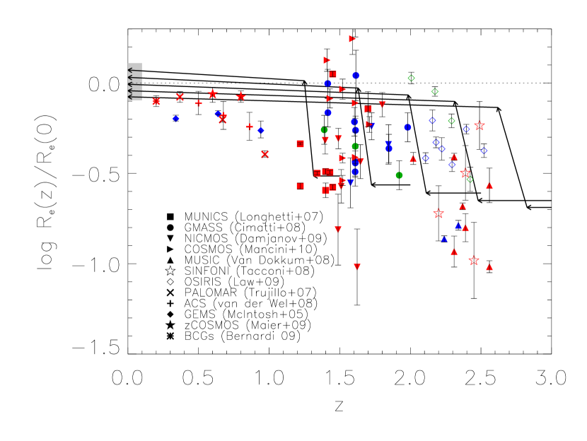
Figure 1.— Evolution of the effective radius with redshift. The data points show: average sizes of $z\lesssim 1$ passively evolving galaxies, divided by the local sizes of galaxies of equal stellar mass, in the samples by Trujillo et al. (2007), McIntosh et al. (2005), van der Wel et al. (2008), Maier et al. (2009) and Bernardi (2009), with the associated errors; individual data and error bars for passively evolving galaxies with spectroscopic redshifts $z\gtrsim 1$ by Longhetti et al. (2007), Cimatti et al. (2008), Damjanov et al. (2009), Mancini et al. (2010), and van Dokkum et al. (2008); data and error bars for individual star forming galaxies with spectroscopic redshifts $z\gtrsim 2$ by Tacconi et al. (2008) and Law et al. (2009). The color of the data points refers to the stellar mass of the galaxy: red is for $M_{\star}\gtrsim 10^{11}\,M_{\odot}$, blue for $3\times 10^{10}\,M_{\odot}\lesssim M_{\star}\lesssim 10^{11}\,M_{\odot}$, and green for $M_{\star}\lesssim 3\times 10^{10}\,M_{\odot}$. The shaded area reflects the distribution of local SDSS galaxies (Hyde & Bernardi 2009). Thick solid lines with arrows illustrate typical evolutionary tracks of massive galaxies according to our reference model (with $f_{\sigma}=1.5$).

2.1. Observed size evolution of passively evolving galaxies

A recent analysis by Maier et al. (2009) of a sample including about 1100 galaxies with Sérsic index $n\gtrsim 2.5$, spectroscopic redshifts in the range $0.5\lesssim z\lesssim 0.9$ and stellar masses in the range $3\times 10^{10}\,M_{\odot}\lesssim M_{\star}\lesssim 3\times 10^{11}\,M_{\odot}$ shows that the size evolution for galaxies at $z\sim 0.7$ is within a factor $f_{r}(0.7)=R_{e}(0)/R_{e}(0.7)\lesssim 1.25$. For galaxies at $0.7\lesssim z\lesssim 0.9$ the size evolution is limited to a factor $f_{r}(0.9)\lesssim 1.4$. Small size evolution ($f_{r}\lesssim 1.3$) for redshifts $z\lesssim 0.8$ was previously reported by McIntosh et al. (2005) for a sample of 728 red galaxies with Sérsic index $n\gtrsim 2.5$ and stellar masses in the range $3\times 10^{9}\,M_{\odot}\lesssim h^{2}\,M_{\star}\lesssim 3\times 10^{11}\,M_{\odot}$; in this case, however, the majority of redshifts were photometric. At lower redshift, $z\approx 0.25$, the Brightest Cluster Galaxies (BCGs) exhibit slow evolution $f_{r}\lesssim 1.3$ (Bernardi 2009).

A size evolution somewhat more pronounced (around $40\%$) than found by Maier et al. (2009) has been claimed by Trujillo et al. (2007) for massive galaxies $M_{\star}\gtrsim 10^{11}\,M_{\odot}$ at redshift $z\approx 0.65$. However, restricting the analysis to galaxies with spectroscopic redshifts in the range $0.5\lesssim z\lesssim 0.8$ (91 galaxies with $n\gtrsim 2.5$ and mean stellar mass of $1.8\times 10^{11}\,M_{\odot}$) we find a mean effective radius of $4.94$ kpc. The mean local effective radius for galaxies with this stellar mass is around $6$ kpc, implying an increase by a factor $f_{r}(0.65)\approx 1.2$. On the other hand, the mean effective radius decreases to $3.8$ kpc for galaxies with the same mean mass but with average redshift $z\approx 0.9$; in this case the size evolution amounts to a factor $f_{r}(0.9)\approx 1.6$. Similar results are found by Ferreras et al. (2009) for a sample of 195 red galaxies selected in the redshift range $0.4\leq z\leq 1.2$. They are, on average, more compact than local galaxies with Sérsic index $n\gtrsim 2.5$ by a factor of only $f_{r}\approx 1.4$.

A stronger evolution of $R_{e}$ at fixed stellar mass was reported by van der Wel et al. (2008) for a composite sample of 50 morphologically selected ETGs in the redshift range $0.8\lesssim z\lesssim 1.2$. Since we are interested on the evolution at $z\lesssim 1$ we have confined ourselves to the 20 galaxies in a massive clusters at $z\approx 0.83$. For these we find, on average, $f_{r}(0.83)\approx 1.6$, but with a substantial mass dependence: the most massive galaxies (dynamical mass within $R_{e}$ of $M_{\rm dyn}\gtrsim 3\times 10^{11}\,M_{\odot}$) fall quite close to the local mass vs. $R_{e}$ relation, while the lower mass galaxies tend to exhibit large size evolution.

All the results mentioned above are shown in Fig. 1, where we also present a compilation of the data at redshift $z\gtrsim 1$. We note that, while the data points at $z\lesssim 1$ are averages over large samples, at higher redshift data points refer to individual galaxies.

Assuming that the average evolution of $R_{e}$ can be described by a power law of the form $R_{e}\propto(1+z)^{\alpha}$, Buitrago et al. (2008) find ${\alpha}=1.48$, while van der Wel et al. (2008) obtain a lower value $\alpha=1.20$. The latter authors also suggest a weaker evolution, corresponding to $\alpha=0.96$, for $z\lesssim 1$. However, even this milder evolution is faster than indicated by the most recent data summarized above, and especially by the most extensive and spectroscopically complete study of Maier et al. (2009).

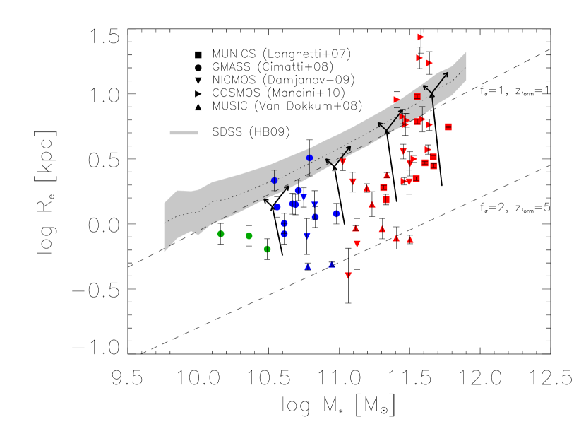
Figure 2.— Correlation between effective radius and stellar mass. The observations of passively evolving galaxies with spectroscopic redshifts $z\gtrsim 1$ by Longhetti et al. (2007), Cimatti et al. (2008), Damjanov et al. (2009), Mancini et al. (2010), and van Dokkum et al. (2008) are compared with the local correlation (Hyde & Bernardi 2009; the dotted line illustrates the average and the shaded area represents the variance). Color code refers to the stellar mass, as in previous Figure. The dashed lines illustrates the outcomes of Eq. (5) for extreme values of the relevant parameters $f_{\sigma}$ and $z_{\rm form}$ (see text). Thick lines with arrows illustrate typical evolutionary tracks of massive galaxies according to our reference model (with $f_{\sigma}=1.5$ and $z_{\rm form}=3$), featuring first the abrupt size growth due to quasar feedback (almost vertical arrows), and then the possible slow size increase due to mass loss (arrows pointing left) or mass additions by minor mergers (right pointing arrows.).

A relevant feature of the data for massive galaxies at high redshift is the quite large spread of the size, as it is apparent from Figs. 1 and 2. Specifically, for masses larger than $10^{11}\,M_{\odot}$ the scatter in size of high redshift ETGs amounts to $\sigma_{log(R_{e})}\approx 0.41$, significantly wider than in local samples, for which we have typically $\sigma_{log(R_{e})}\approx 0.14$ (cfr. Shen et al. 2003; Hyde & Bernardi 2009). In more detail, several high redshift galaxies exhibit the same size as their local counterparts (see e.g. Mancini et al. 2010; Onodera et al. 2010), while about half ETGs exhibit $f_{r}\gtrsim 3-4$, with several of them having $f_{r}\gtrsim 8-10$. It is worth noticing that Maier et al. (2009) find for the size distribution at fixed mass of their sample of ETGs at redshift $\approx 0.7$ a statistical dispersion $\sigma_{log(R_{e})}\approx 0.16$ very close to the local one.

Provided that the presently available data constitute a representative sample of the size of high redshift ETGs, both the average increase of the size and the narrowing of its distribution are to be accounted for. Only large samples of high-$z$ ETGs will allow us to assess the interesting issue of their size distribution. We also note that the paucity of data at $z\gtrsim 1$ prevents the investigation of the possible mass dependence, a crucial aspect for any interpretation of the phenomenon.

So far we have discussed the evolution by comparing high redshift size determinations with the average size of local ETGs. A bias may arise because high-$z$ samples of passively evolving galaxies pick up objects that formed at higher redshifts and therefore have smaller sizes. The majority of local ETGs probably formed at $1.5\lesssim z_{\rm form}\lesssim 2.5$, but ETG progenitors already in passive evolution at $z\approx 2-2.5$ formed about $1$ Gyr earlier, i.e., at $z_{\rm form}\gtrsim 3.5$. The latter are expected to have, on average, a factor $\approx 1.5-2$ smaller size than local ETGs (see Eq. 2.3 below). This may explain why Valentinuzzi et al. (2010) find that a substantial fraction (around $22\%$) of ETGs in local galaxy clusters (overdense regions were the galaxies typically formed earlier than in the field) are more compact than the local average. In fact, their cluster galaxies are on average $1.5$ Gyr older than local ETGs with ‘normal’ size. It is worth mentioning that several massive blue galaxies have recently been found to exhibit compact sizes (Trujillo et al. 2009).

2.2. Sizes of high-redshift star forming galaxies

Massive starforming galaxies at high-$z$ are heavily obscured by dust and therefore their structure cannot be investigated by means of optical or near-IR observations; however, one can resort to interferometric observations at millimeter and submillimeter wavelengths. In particular CO molecular emission has been spatially resolved for a sample of submillimeter bright galaxies at $z\approx 2$ by Bouché et al. (2007) and Tacconi et al. (2008, 2010) with the IRAM Plateau de Bure millimeter interferometer. The results obtained for the galaxies with spectroscopic redshift are shown in Fig. 1. For these objects the dynamical mass is a good proxy for the mass in stars and gas.

In Fig. 1 we also plotted the data of Law et al. (2009) on a sample of Lyman break galaxies at redshifts $2\lesssim z\lesssim 3$ and with kinematics dominated by random motions at least in the central $2-3$ kpc. In this case, $R_{e}$ refers to the $H\alpha$ or [OIII] emissions, which are sensitive to dust extinction. The light distribution is expected to be irregular and knotty, as in fact it is observed. Since the dust distribution inside starforming galaxies follows the star and gas distributions, which peak in the central regions, we expect that the observed light profile is broadened with respect to the true star and gas distribution for rest-frame wavelengths shorter than a few microns (see Joung et al. 2009). Therefore the estimated half-light radii of $H\alpha$ or [OIII] emissions should be considered as upper limits. Nevertheless, Fig. 1 suggests that large starburst galaxies and high-$z$ passively evolving galaxies, their close descendants, exhibit the same trend of smaller size with respect to the local ETGs.

2.3. Expected sizes of high redshift galaxies

Caon et al. (1993; see also Kormendy et al. 2009) showed that the Sérsic (1963) function:

$$I(r)=I(0)\,e^{-b_{n}\,(r/R_{e})^{1/n}}~{},$$ (1)

fits the brightness profiles of nearly all ellipticals with remarkable precision over large dynamic ranges. Here $I(0)$ is the central surface brightness, $R_{e}$ is the half-luminosity radius, and $n$ is the Sérsic’s index. The constant $b_{n}$ can be determined from the condition that the luminosity inside $R_{e}$ is half the total luminosity $L(R_{e})=L_{T}/2$ (see Prugniel & Simien 1997). The classical de Vaucouleurs (1953) profile corresponds to $n=4$.

If light traces mass, the projected half stellar mass radius $R_{e}$ is related to the gravitational radius $R_{g}$ by $R_{e}=S_{s}(n)\,R_{g}$, and the density-weighted, $3-$dimensional velocity dispersion $\sigma_{\star}$ is related to the observed line-of-sight central velocity dispersion $\sigma_{0}$ by $\sigma_{\star}=[3\,S_{K}(n)]^{1/2}\,\sigma_{0}$. Note that $\sigma_{0}$ is usually measured within a physical size of about $0.1\,R_{e}$ (e.g., Jørgensen et al. 1993). At virial equilibrium, the mass is given by:

$$M_{\star}=S_{D}(n)\frac{1}{G}\,R_{e}\,\sigma_{0}^{2}~{}$$ (2)

where $S_{D}(n)=3\,S_{K}(n)/S_{s}(n)$. Prugniel & Simien (1997) have tabulated the coefficients $S_{D}$, $S_{K}$, and $S_{s}(n)$ for values of the Sérsic index $n$ ranging from $1$ to $10$; in particular, $S_{s}(4)\approx 0.34$, $S_{K}(4)\approx 0.52$, and $S_{D}(4)=4.591$.

The stellar component gravitationally dominates in the inner regions of galaxies, while the DM with its extended halo dominates in the outer regions. To a halo with mass $M_{\rm H}$ we can associate an initial baryon mass $M_{\rm b,i}=f_{b}\,M_{\rm H}$, where $f_{b}\approx 0.2$ is the cosmic baryon to DM mass ratio. Weak lensing observations (Mandelbaum et al. 2006), extended X-ray emission around ETGs (e.g., O’Sullivan & Ponman 2004) and the comparison of the statistics of the halo mass function with the galaxy luminosity function (Vale & Ostriker 2004; Shankar et al. 2006; Guo & White 2009; Moster et al. 2010) point to a present-day ratio $m=M_{\rm H}/M_{\star}\approx 20-40$ between the total halo mass to the total mass in stars for red massive galaxies. This result quantifies the inefficiency of the star formation process even in large galaxies, since $M_{\star}/M_{\rm b,i}=1/(m\,f_{b})$. The dependence of $m$ on mass and redshift predicted by our reference model (Granato et al. 2004) is discussed in the Appendix.

As for the inner regions, we consider the ETG progenitor $1255-0$ at $z\approx 2.2$, for which van Dokkum et al. (2009) and Kriek et al. (2009) find $M_{\star}\approx 2\times 10^{11}\,M_{\odot}$ within the half-light radius $R_{e}\approx 0.8$ kpc; local ETGs with the same mass have an average size $R_{e}\approx 7$ kpc (see Shen et al. 2003; Hyde & Bernardi 2009). If $m\approx 30$, we can associate to $1255-0$ a halo mass $M_{\rm H}\approx 6\times 10^{12}\,M_{\odot}$. Assuming a NFW profile with concentration $c=4$, it is easy to see that inside the gravitational radius $R_{g}\approx 3\,R_{e}\approx 3$ kpc, the DM fraction amounts to $f_{\rm DM}\approx 0.1$. We notice that the DM contribution to the mass within the half-light radius $R_{e}$ of local ETGs is $f_{\rm DM}\lesssim 30\%$ (e.g., Borriello et al. 2003; Tortora et al. 2009, Cappellari et al. 2006), and has a small effect on the stellar velocity dispersion. This supports the notion that the dissipationless DM cannot parallel the dissipative collapse of baryons, so that its gravitational effects within $R_{e}$ can be neglected also during the compact phase of galaxy evolution.

After the dissipative collapse of baryons inside a host DM halo, the gravitational radius of the baryonic component, stars plus gas with mass $M_{\star}$ and $M_{\rm gas}$ respectively, reads

$$R_{g}=\frac{G\,M_{\star}\left(1+f_{\rm gas}\right)}{\sigma_{\star}^{2}}$$ (3)

where $f_{\rm gas}=M_{\rm gas}/M_{\star}$ is the gas to star mass ratio within the gravitational radius. We note that the central gas mass includes the cold component as estimated in the Appendix (see Eq. [A4] and below for analytic approximations).

If before collapse the baryons had the same velocity dispersion $\sigma_{\rm b,i}$ as the DM $\sigma_{\rm DM}$, and taking into account that $\sigma_{\rm DM}$ is approximately equal to the halo rotational velocity $V_{\rm H}$ (see Appendix), the 3-D stellar velocity dispersion $\sigma_{\star}$ at the end of the collapse can be written as (Fan et al. 2008):

$$\sigma_{\star}=f_{\sigma}\,\sigma_{\rm b,i}=f_{\sigma}\,\sigma_{\rm DM}\approx f_{\sigma}\,V_{\rm H}~{}.$$ (4)

Recalling that $R_{e}=S_{s}(n)\,R_{g}$, with $R_{g}$ given by Eq. (3), and that $V_{\rm H}^{2}=G\,M_{\rm H}/R_{\rm H}$ we then obtain $R_{e}$ in terms of the halo radius $R_{\rm H}$ and mass $M_{\rm H}$:

$$R_{e} \approx \frac{S_{s}(n)}{f_{\sigma}^{2}}\,\frac{\left(M_{\star}+M_{\rm gas}\right)}{M_{\rm H}}\,R_{\rm H}\approx$$

$$\approx 0.9\,\frac{S_{s}(n)}{0.34}\,\frac{25}{m}\,\left(\frac{1.5}{f_{\sigma}}\right)^{2}\,\left(\frac{M_{\rm H}}{10^{12}\,M_{\odot}}\right)^{1/3}\,\left(\frac{4}{1+z_{\rm form}}\right)~{}~{}~{}\mathrm{kpc},$$

where $z_{\rm form}$ is the redshift when the collapse begins, and we have set $f_{\rm gas}=1$. This equation shows that the baryon collapse naturally leads to kpc or sub-kpc effective radii and to stellar velocity dispersions higher than halo rotational velocities ($f_{\sigma}>1$). Both these properties differ from those observed for local massive galaxies, implying that other ingredients have come into play.

The explicit redshift dependence of $R_{e}$ in Eq. (2.3) comes from the halo radius, which scales as $(1+z_{\rm form})^{-1}$. In addition, the ratio $m$, which measures the star formation inefficiency and is determined by the physics of baryons, scales as $(1+z_{\rm form})^{-0.25}$ (see Appendix). As a result the effective radius scales like $R_{e}\propto(1+z_{\rm form})^{-0.75}$. The values of $m$ and of $f_{\sigma}$ depend on how and when the star formation and gas heating processes can halt the collapse. The latter must proceed at least until the mass inside the $R_{e}$ is dominated by stars, as observed in local ETGs.

In Fig. 2 we compare the observed distribution of local and high-$z$ galaxies in the $R_{e}$ vs. $M_{\star}$ plane with expectations from Eq. (2.3). A robust upper limit to the high-$z$ correlation (upper dashed line in Fig. 2) is obtained setting $f_{\sigma}=1$ (baryon collapse with no increase of the stellar velocity dispersion) and $z_{\rm form}=1$, corresponding to a look-back time of about $7-8$ Gyr, a lower limit to the mass-weighted age of local massive ETGs (Gallazzi et al. 2006; Valentinuzzi et al. 2010). The corresponding line falls just at the lower boundary of the distribution of local ETGs, but at the upper boundary of the distribution of high-$z$ passively evolving massive galaxies. The median size of the latter is a factor around $4$ lower than that of local galaxies with the same stellar mass. This argument is not in contrast with the existence, recently reported by Valentinuzzi et al. (2010), of local compact ETGs, which can represent the evolution of the oldest, most compact progenitors.

The lower bound to the high-$z$ correlation is less well defined; in Fig. 2 the lower dashed line corresponds to $z_{\rm form}\sim 5$ and to $f_{\sigma}=2$. In Eq. (2.3), we have adopted as our reference values $f_{\sigma}=1.5$ and $z_{\rm form}=3$.

3. Evolution of the ETG velocity dispersions

Applying the virial theorem to the galaxies before and after their growth in size, we have that the final line of sight central stellar velocity dispersion $\sigma_{\rm 0,f}$ is related to the initial one $\sigma_{\rm 0,i}$ by:

$$\sigma_{0,f}^{2}=\sigma_{0,i}^{2}\,\frac{S_{D}(n_{i})}{S_{D}(n_{f})}\,\frac{M_{f}}{M_{i}}\,\frac{R_{e,i}}{R_{e,f}}=\frac{f_{\sigma}^{2}\,V^{2}_{\rm H}(z_{\rm form})}{3\,S_{K}(n_{i})}\,\frac{S_{D}(n_{i})}{S_{D}(n_{f})}\,\frac{M_{f}}{M_{i}}\,\frac{R_{e,i}}{R_{e,f}}~{};$$ (6)

here the indices $i$ and $f$ label quantities in the initial and final configuration, and $S_{D}(n)$ is the structure factor defined by Prugniel & Simien (1997; see Eq. [2]), $n$ being the Sérsic index. In the last expression we have used Eq. (4) and the relation $\sigma_{\star}^{2}=3\,S_{K}(n_{i})\,\sigma_{0,i}^{2}$. In the case of an homologous growth of the galaxy size, the velocity dispersion scales as $(M/r)^{1/2}$, so that it remains constant if both the mass and the size increase by the same factor and decreases as $r^{-1/2}$ if the growth occurs at constant mass. However, the size growth is not necessarily homologous. All the mechanisms so far proposed predict an increase of the Sérsic index with increasing size. This effect together with a possible increase in mass within the limits imposed by the mass function evolution, tend to soften the decrease of the velocity dispersion. A further attenuation of the evolution is expected because of dynamical friction with the DM component.

The above equation shows that the size evolution of ETGs is paralleled by velocity dispersion evolution and that the present-day velocity dispersion keeps track of the potential well of the host halo when the galaxy forms. This is expected, since in a galaxy halo the gas is channeled toward the central regions during the fast accretion phase under the effect of the DM potential well. The duration of the star formation process depends on halo mass, feedbacks and redshift at which the fast accretion phase occurs. The velocity dispersion of the collapsed galaxy is not affected by the minor fraction of DM added subsequently to the external regions of a halo during the slow accretion phase (see Lapi & Cavaliere 2009).

Observations of the kinematics of passively evolving ETGs at $z\gtrsim 1$ are quite difficult. Nonetheless for two galaxies reliable estimates of the velocity dispersion have been obtained (Cappellari et al. 2009; van Dokkum et al. 2009). For other objects only average estimates have been inferred from stacked spectra (Cenarro & Trujillo 2009; Cappellari et al. 2009). In all cases the main conclusion is that stellar masses derived from spectrophotometry are in good agreement with virial masses or with masses derived from dynamical models, if one adopts an IMF flattening below $1\,M_{\odot}$, such as those proposed by Kroupa (2001) or by Chabrier (2003). This finding is also confirmed at intermediate redshifts $0.4\lesssim z\lesssim 0.9$ by van der Wel et al. (2008).

One of the two high redshift ETGs with a good determination of the velocity dispersion, GMASS 2470 (Cappellari et al. 2009), falls in the $\sigma$ vs. $R_{e}$ plane quite close to the area covered by local ETGs. On the other hand, the best fit value of the stellar velocity dispersion, $\sigma_{0}=510^{+165}_{-95}$, for the galaxy 1255-0 at $z\approx 2.2$ (van Dokkum et al. 2009) exceeds the measured values for even the most massive local galaxies (Bernardi et al. 2008). Although we cannot do statistics with a single case, its existence lends support to the possibility of a significant evolution of the galaxy velocity dispersion.

Cappellari et al. (2009; see also Bernardi 2009), based on stacked spectra of $13$ galaxies at $1.4\lesssim z\lesssim 2.0$ (cf. their Table 1), find a mild evolution of the velocity dispersion, that decrease from about $202$ km s^-1 at $z\approx 1.6$ down to about $160$ km s^-1 at $z\approx 0$ for $M_{\star}\approx 7\times 10^{10}\,M_{\odot}$, and find an increase of the source size by a factor around $3.5$. This evolution can be understood if the Sérsic’s index $n$ increases from an initial value $n_{i}$ to $n_{f}=n_{i}+2$ and the mass increases by $30\%$; in that case the velocity dispersion decreases by a factor $1.35$, or less if dynamical friction with DM has a role. Note that if, as shown in § 2.3, the DM is dynamically irrelevant in the inner regions of galaxies, and mergers accrete matter in the outer regions, the mass within $R_{e}$ does not change and the same velocity dispersion evolution applies also to the minor merger scenario.

A quite interesting upper limit to the velocity dispersion, $\sigma_{\star}\lesssim 326$ km s^-1, for a massive $M_{\star}\approx 3-4\times 10^{11}\,M_{\odot}$ at redshift $z\approx 1.82$ has been found by Onodera et al. (2010). The same authors also find that the size of this galaxy is as expected for a local galaxy with the same mass. The velocity dispersion and the size yield a virial mass upper limit $M_{H}\lesssim 7\times 10^{11}\,M_{\odot}$, quite close to the stellar mass. This galaxy has the same structural properties of a local ETG. Recalling that a significant fraction of $z\gtrsim 1.5$ galaxies already exhibit a size close to the size of their local counterparts, this galaxy appears as a well studied case of an already evolved galaxy, suggesting that the timescale for the size evolution is shorter than the Hubble time at those redshifts $\Delta T_{\rm size}<t_{H}(z)$.

4. Physical mechanisms for size evolution

Both theory and observations suggest that at least $60\%$ of ETGs evolve in size by at least a factor of $2-4$. So far, two main mechanisms have been proposed to accomplish such evolution. One possibility is that the expansion is driven by the expulsion of a substantial fraction of the initial baryons, still in gaseous form, by quasar activity (Fan et al. 2008) or by an expulsion of gas associated to stellar evolution (e.g., Damjanov et al. 2009). The two mechanisms differ in the expulsion timescale, which is shorter than the dynamical time if it is triggered by quasar activity and longer in the case of ejection associated to stellar evolution (with ‘standard’ IMFs).

Alternatively, the increase in size could be due to minor mergers on parabolic orbits that add stars in the outer parts of the galaxies along the cosmic time from $z\approx 1-2$ to the present epoch (see Maller et al. 2006; Naab et al. 2009; Hopkins et al. 2009b; van der Wel et al. 2009). Major mergers (i.e., mergers of galaxies with similar mass) can also increase the galaxy size in a way almost directly proportional to the mass increase and they were also considered (e.g., Boylan-Kolchin et al. 2006; Naab et al. 2007) but the required space densities of progenitors were found to be incompatible with the present-day galaxy mass function (Bezanson et al. 2009; Toft et al. 2009) as well as with the dearth of compact, massive galaxies in the local universe (Trujillo et al. 2009).

A third possibility is that the increase is illusory, because the low-surface brightness in the outer regions of high-$z$ galaxies may be missed and the effective radii are correspondingly underestimated (Mancini et al. 2010; Hopkins et al. 2010) or because a gradient in the $M/L$ ratio (lower in the bluer central regions) can make the half-light radius in the optical smaller than the half-mass radius (Tacconi et al. 2008); however, Szomoru et al. (2010) find no evidence of outer faint envelopes in a well-studied galaxy at $z\approx 1.9$.

4.1. Gas expulsion

In the case of gas expulsion the final size depends on the timescale of the ejection itself. If the ejection occurs on a timescale shorter than the dynamical timescale of the system $\tau_{\rm ej}<\tau_{\rm dyn}$, immediately after the ejection the size and velocity dispersion are unchanged but the total energy is larger because the mass has decreased. The system then expands and evolves towards a new equilibrium configuration. In the case of homologous expansion the final size $R_{f}$ is related to the initial one $R_{i}$ by (Biermann & Shapiro 1979; Hills 1980):

$$\frac{R_{i}}{R_{f}}=1-\frac{M_{\rm ej}}{M_{f}}$$ (7)

where $M_{\rm ej}$ is the ejected mass and $M_{f}$ is the final mass.

This simple result has been confirmed by numerical simulations of star clusters (e.g., Geyer & Burkert 2001; Boily & Kroupa 2003). In particular, the simulations by Goodwin & Bastian (2006) and by Baumgardt & Kroupa (2007) show that the expansion of the half-mass radius occurs in about $20$ dynamical times and the new final equilibrium is attained within $40$ dynamical times. We note that the case of galaxies differs from that of the star clusters owing to the presence of the DM halo. In ETGs the DM halo exerts its gravitational influence outside the central region dominated by stars and prevents the galaxy disruption when $M_{\rm ej}$ approaches or exceeds $M_{f}$; the DM potential can also influence the time taken by the stars to reach the new equilibrium.

When the mass loss occurs on a timescale longer than the dynamical time the system expands through the adiabatic invariants of the stellar orbits and one gets

$$\frac{R_{f}}{R_{i}}=1+\frac{M_{\rm ej}}{M_{f}}~{}.$$ (8)

Comparison of the two above equations show that the fast expulsion is more effective in increasing the size.

The dynamical time of the stellar component is

$$\tau_{\rm dyn}=\pi\,\left(\frac{R_{e}^{3}}{2\,G\,M_{\star}}\right)^{1/2}\approx 3\times 10^{6}\,\left(\frac{R_{e}}{1~{}\rm kpc}\right)^{3/2}\left(\frac{10^{11}\,M_{\odot}}{M_{\star}}\right)^{1/2}~{}\mathrm{yr},$$ (9)

about $30-50$ times shorter than the typical dynamical timescale in local massive ETGs and not much longer than the dynamical timescale usually associated to star clusters. In the case of mass loss due to stellar feedback (Hills 1980; Richstone & Potter 1982) $\tau_{\rm ej}\gg\tau_{\rm dyn}$ for any reasonable choice of the IMF. For instance, if a Chabrier (2003) or Kroupa (2001) IMF is adopted, after an initial burst about half of the mass of formed stars returns to the gaseous phase over a timescale of $1$ Gyr. If this gas is removed from galaxies, the size may grow by a factor of about $2$. The higher the proportion of massive stars, the larger the effect on the size, and the shorter the timescale for the size expansion (see Damjanov et al. 2009).

In the case of quasar winds the typical timescale for gas ejection can be estimated as

$$\tau_{\rm ej}=\frac{M_{\rm gas}}{\dot{M}_{\rm wind}} \approx 5\times 10^{6}\,\left(\frac{m}{25}\right)^{2/3}\,\left(\frac{M_{\star}}{10^{11}\,M_{\odot}}\right)^{5/3}\times$$ (10)

$$\times \left(\frac{M_{\bullet}}{2\times 10^{8}\,M_{\odot}}\right)^{-3/2}\,\left(\frac{1+z}{4}\right)~{}\mathrm{yr},$$

where $\dot{M}_{\rm wind}$ is given by Eq. (A12), and we have assumed $M_{\rm gas}\approx M_{\star}$. An alternative definition of $\tau_{\rm ej}$ is

$$\tau_{ej}=\frac{R_{e}}{V_{e}}\approx 10^{6}\,\left(\frac{R_{e}}{1\,\mathrm{kpc}}\right)^{1/2}\,\left(\frac{M_{\star}}{10^{11}\,M_{\odot}}\right)^{-1/2}\,\mathrm{yr}~{},$$ (11)

where $V_{e}^{2}=2\,G\,M_{\star}/R_{e}$ is the escape velocity from the radius $R_{e}$. With both definitions the ejection timescale is of the order of the dynamical timescale.

It is apparent that numerical simulations are badly needed to investigate the detailed effect of quasar winds on the size and on the timescale $\Delta T_{\rm size}$ to reach the new equilibrium; such kind of simulations are underway (L. Ciotti and F. Shankar 2009, private communication).

4.2. Minor mergers

In the case of minor mergers on parabolic orbits the initial potential energy of the accreting mass is neglected in the computation. Following Naab et al. (2009) we assume that random motions are dominant in high-$z$ ETG precursors and set $\eta=M_{a}/M_{i}$ and $\epsilon=\sigma^{2}_{a}/\sigma^{2}_{i}$, the $i$ and $a$ indices referring to initial and accreted material. The mass after merging is therefore $M_{f}=M_{i}\,(1+\eta)$. If $r\propto M_{\star}^{\alpha}$, the virial theorem gives $\epsilon=\eta^{1-\alpha}$. Local ETGs have $\alpha\approx 0.56$ (Shen et al. 2003) or even larger in the case of BCGs (Hyde & Bernardi 2009); in addition, a value $\alpha\approx 0.5$ is implied by the Faber-Jackson (1976) relationship.

From the virial theorem and the energy conservation equation it is easily found that the fractional variations of the gravitational radius and of the velocity dispersion between the configurations before ($i$) and after ($f$) merging are:

$$\frac{R_{g,f}}{R_{g,i}}=\frac{(1+\eta)^{2}}{(1+\eta^{2-\alpha})}~{},$$

(12)

$$\frac{\sigma_{f}^{2}}{\sigma_{i}^{2}}=\frac{(1+\eta^{2-\alpha})}{(1+\eta)}~{}.$$

Boylan-Kolchin et al. (2008) showed that minor mergers can be effective only if $\eta\gtrsim 0.1$, lower mass ratios requiring too long timescales.

Recent numerical simulations by Naab et al. (2009) agree with these results. Their simulated galaxy, with a mass in stars $M_{\star}\approx 8\times 10^{10}\,M_{\odot}$ and half-mass radius $R_{e}\approx 1$ kpc at $z\approx 2$, by $z=0$ has doubled its stellar mass through minor mergers, reaching $M_{\star}\approx 1.5\times 10^{11}\,M_{\odot}$, while the half-mass radius has increased by a factor $2.7$. The simulations also suggest that most of the increase, a factor of about $1.8$, occurs at $z\lesssim 1$, i.e, on a cosmological timescale. This is accompanied by a moderate decrease, $\lesssim 20\%$, of the central velocity dispersion between $z\approx 3$ and $z\approx 0$ and by a decrease of the central density of stellar distribution with time, due to dynamical friction, despite of the total mass increase. However, these simulations yield a present-day half-mass radius a factor of $2$ smaller than expected on the basis of the $M_{\star}$ vs. $R_{e}$ relationship of Shen et al. (2003; see also Fig. 2).

We notice that the size evolution in the merging case occurs on timescale which is comparable with the present Hubble time with size scaling $\propto(1+z)^{\beta}$; in the simulations of Naab et al. (2009) $\beta\approx 1$ holds, and similarly in the findings of van Dokkum et al. (2010) $\beta\approx 1.27$.

5. Discussion

The observational data and the theoretical arguments summarized in the previous sections allow us to test and constrain the different models for size evolution. Since a size increase by minor dry mergers implies an increase in mass, we start by discussing limits on the latter.

5.1. The mass evolution of ETGs

Spectral properties of local ETGs with stellar masses $M_{\star}\gtrsim 3\times 10^{10}\,M_{\odot}$ indicate that their light-weighted age exceeds $8-9$ Gyr, independently of the environment (see Renzini 2006 for a review and Gallazzi et al. 2006 for an extensive statistical study). Since light-weighted ages are lower limits to mass-weighted ages (e.g., Valentinuzzi et al. 2010), it is generally agreed that most of the stars of massive ETGs formed at $z_{\rm form}\gtrsim 1.5-2$. An upper limit $\lesssim 25\%$ to the fraction of stars formed in ETGs in the last $\approx 8$ Gyr, and as a consequence to the fraction of gas accreted at intermediate redshift $z\lesssim 1$, has been derived from studies of narrow band indices of local field ETGs (e.g., Annibali et al. 2007). Moreover, all massive galaxies that formed and gathered the bulk of their stars at $z\gtrsim 1$ are presently ETGs or massive bulges of Sa galaxies, since there are no late-type, disc-dominated galaxies endowed with so large masses of old stellar populations.

Thus by comparing the stellar mass function of local ETGs to the mass function of all galaxies at $z\lesssim 1.5$, we can derive information on the mass evolution.

Bernardi et al. (2010) studied in detail about $2000$ morphologically-classified local galaxies extracted from the SDSS sample (see Fukugita et al. 2007). They showed that the concentration index $C_{r}$ can be used to discriminate among galaxy types. The criterion $C_{r}>2.86$ includes almost all ellipticals, about 80$\%$ of S$0$ galaxies and 40$\%$ of Sa galaxies, likely those with a larger disk component of younger and bluer stars. Correspondingly, while the fraction of E and S0 massive galaxies ($M_{\rm dyn}\gtrsim 10^{11}\,M_{\odot}$) older than $8$ Gyr is quite large, the fraction of massive and old Sa galaxies is less than $50\%$ (cf. Fig. 23 of Bernardi et al. 2010).

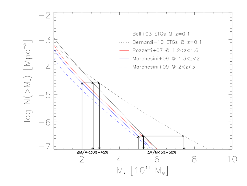
Figure 3.— Cumulative stellar mass function. The different lines illustrate Schechter fits to the average stellar mass function at different redshifts as estimated by Bell et al. (2003), Bernardi et al. (2009), Pozzetti et al. (2007), and Marchesini et al. (2009). All estimates have been scaled to Chabrier’s (2003) IMF. Thick solid lines with arrows highlight the mass evolution from $z\approx 1.5$ to the present allowed by the observed mass functions, starting from $M_{\star}\approx 2$ and $5\times 10^{11}\,M_{\odot}$.

Therefore, in order to consistently compare the high redshift mass function with the local one, in Fig. 3 we report the cumulative mass function for the full Bernardi et al. (2010) sample with concentration index $C_{r}>2.86$. We also plot the mass function by Cole et al. (2001; similar results were obtained by Bell et al. 2003), that has been computed with criteria that tend to exclude late type galaxies. These local mass functions are compared with estimates by Pozzetti et al. (2007) and Marchesini et al. (2009), which refer to redshift $z\approx 1.4$ and $z\approx 1.6$, respectively. All mass functions have been rescaled to Chabrier’s (2003) IMF.

When comparing the local to the high redshift ETG mass function, the first issue is how to make a complete census of high redshift ETG progenitors. Williams et al. (2009) found that in a deep sample (magnitudes $K_{\rm AB}<22.4$) the most luminous objects at $z\sim 1-2$ are divided roughly equally between starforming and quiescent galaxies. A significant fraction of galaxies at $z\gtrsim 1.5$, forming stars at rates of hundreds to thousands solar masses per year as revealed by far-IR or submillimeter surveys, are easily missed even by deep $K-$band surveys because of their strong dust obscuration (e.g., Dye et al. 2008). An extreme example is GN10, a galaxy at $z\approx 4$ that exhibits a star formation rate around $1000\,M_{\odot}$ yr^-1, a stellar mass around $10^{11}\,M_{\odot}$ and a dust extinction $A_{V}\sim 5-7.5$ mag (see Daddi et al. 2009; Wang et al. 2009); this went undetected by ultradeep $K_{s}-$band exposures, yielding a $1-\sigma$ upper limit of 23 nJy (Wang et al. 2009) that corresponds to $K_{\rm AB}\gtrsim 28$. Since all galaxies at redshift $z\gtrsim 1.5$ have to be included in the budget, mass functions of high redshift massive galaxies based on optical or near-IR selected samples should be regarded as lower limits to the high redshift counterparts of local ETGs (see Silva et al. 2005 for a more detailed discussion). As a consequence, only upper limits to evolution in mass allowed by the data obtains by assuming that the galaxy number density keeps constant.

In addition, it is apparent from Fig. 1 of van Dokkum et al. (2010) that the upper limit to mass evolution slightly depends on mass or correspondingly on the reference number density. van Dokkum et al. (2010) adopt as a reference number density $2\times 10^{-4}$ Mpc^-3 dex^-1 and find that galaxies with this number density at $z\approx 1.6$ are endowed with $M_{\star}\approx 1.7\times 10^{11}\,M_{\odot}$, while at $z\approx 0.1$ the same number density pertains to galaxies with $M_{\star}\approx 2.8\times 10^{11}\,M_{\odot}$ (the adopted local number density is that of Cole et al. 2001); the ensuing upper limit to mass evolution is $\lesssim 70\%$. Applying the same argument to galaxies with number density $2\times 10^{-5}$ Mpc^-3 dex^-1 yields an upper limit to mass evolution $\lesssim 40\%$. If the local number density of Bernardi et al. (2010) is adopted, the upper limit to mass evolution is $\lesssim 50\%$ since $z\approx 1.6$ with practically no dependence on mass, as shown in Fig. 3.

These upper limits are compatible with evidences that most, if not all, massive ETGs are already in place at redshift $z\approx 1$ (see Drory et al. 2005; Pérez-González et al. 2008; Fontana et al. 2006; Cirasuolo et al. 2010; Kajisawa et al. 2009) and that only a fraction $\lesssim 30\%$ of their stellar mass can be added at later times. Collins et al. (2009) have estimated the masses of the Brightest Cluster Galaxies (BCGs) in $5$ of the most distant X-ray-emitting galaxy clusters at redshifts $z\sim 1.2-1.5$, finding that they are perfectly compatible with the local average mass of BCGs. If the two galaxies, which have companions, incorporated them, their mass would increase in one case by about $20\%$ and in the other by $40\%$.

The results of numerical simulations on DM halos are compatible with such a mass increase. More in detail, Boylan-Kolchin et al. (2008) showed that only merging of satellites with mass ratio $\eta\gtrsim 0.1$ can efficiently increase the mass of their host galaxies. Also the merging rate for massive galaxies inferred from numerical simulations by Stewart et al. (2008) confirms that most of the mass is added by merging of satellites with mass ratio $\eta\gtrsim 0.1$. We stress, however, that these simulations refers to the DM halos and its translation to stellar component of merging halos is not trivial.

To sum up, the data allow, at most, for a mass increase by a factor of $\approx 2$ since $z\approx 2$ and by a factor of $\approx 1.5-1.7$ since $z\approx 1.5$. We notice also that if the growth occurs via minor dry mergers, with no evolution of the galaxy number density, practically all massive galaxies gradually increased their mass throughout their entire lifetime, from the formation redshift to $z=0$ [see, e.g., the simulations by Naab et al. (2009) and Stewart et al. (2008)]. But then also the galaxy sizes should increase gradually over the full galaxy lifetime, and this can be hardly reconciled with the much larger scatter in size observed for ETG progenitors at $z\gtrsim 1.5$ compared to that at lower redshifts.

5.2. Size evolution

The comparison of available data on $z\gtrsim 1$ ETGs with the local size distribution clearly points toward a mean size increase by about a factor of $3$ in order to bring the average $M_{\star}$ vs. $R_{e}$ relationship of high redshift ETGs to the local average (cf. Fig. 1), though we caution that larger samples of high redshift ETGs are needed. We stress that the observed small sizes at high-$z$ are indeed expected (cf. Eq. [2.3]) if ETG progenitors formed most of their stars in a rapid, dissipative collapse.

As a matter of fact, we expect that high redshift passively evolving ETGs formed at redshift $z_{\rm form}\gtrsim 4$ larger than the formation redshift $z_{\rm form}\approx 1.5-2$ of most local ETGs. From the number density of halos with $M_{\rm H}\gtrsim 10^{12}\,M_{\odot}$ as a function of redshift, we estimate that massive galaxies (with $M_{\star}\gtrsim 10^{11}\,M_{\odot}$) formed at redshift $z_{\rm form}\gtrsim 4$ are only $10\%$ of those formed at $z_{\rm form}\approx 2$. Therefore, since $R_{e}\propto(1+z_{\rm form})^{-0.75}$ (see § 2.3), the local counterparts of high-$z$ ETGs, $10\%$ of the total number of ETGs, are expected to exhibit a half-light radius smaller than the average by a factor around $1.4$.

Taking into account this bias, data in Fig. 1 and in Fig. 2 show that a significant fraction of local ETG precursors already at $z\gtrsim 1.5$ exhibit the same size as their local counterparts of the same mass. On the other hand, there are also ETG progenitors much more compact than their local counterparts, with sizes smaller by a factor $\lesssim 1/6$. As a matter of fact, the dispersion in size at high redshift is larger than in the local samples of ETGs. These properties of the size distribution can be accounted for by a model yielding evolution in size by large factors ($\gtrsim 5$) on timescales shorter than the Hubble time $t_{H}$ at $z\gtrsim 1.5$. Ejection of large amounts of gas by quasar feedback can reproduce the observed phenomenology. From Eq. (7) it is apparent that large size expansions are possible, even though gravity of DM halos will constrain them. Also from Eq. (9) it is apparent that timescales from a few to several $10^{8}$ yr can be required for the expansion. In this context the scatter of sizes mirrors the spread of formation time and the spread in the expansion phase, as illustrated by Fig. 1 and Fig. 2. In particular, in Fig. 1 lines with an arrow represent the size evolution predicted by our reference model. The lower horizontal lines represent the time (translated to $\Delta z$) spent by ETG progenitors in their dusty phase with quite large star formation rate; submm surveys are quite efficient in selecting this phase. Then the (almost vertical) lines represent the epoch of the large size increase due to the gas outflow triggered by the quasar activity; this phase begins with the quasar appearance and lasts $\Delta T_{\rm size}$ (here $\Delta T_{\rm size}\approx 2\times 10^{8}$ yr has been assumed). Then a longer phase lasting for about the present Hubble time follows, during which the size can increase by a smaller factor because of mass loss due to galactic winds and/or minor dry mergers.

We note that quasar feedback has not been introduced specifically to solve the size problem, but first by Silk and Rees (1998) to predict the correlation in ETGs between galaxy velocity dispersion and the present-day BH mass. Soon after, Granato et al. (2001, 2004) have shown that the gas removal by quasar activity is also needed in order to stop the star formation, preventing formation of exceedingly massive galaxies, too blue and with no enhancement of $\alpha$-elements (cf. § 5.1). Sterilization of star formation by quasar feedback implies that in a quite short timescale, an enormous mass of gas is evacuated from the central galaxy regions and possibly from the entire halo and subhalos. The gas evacuated from the central regions can be of the same order of the mass in stars, so about $10-20\%$ of the total baryons in the galactic halo. Observations of high redshift star forming galaxies do find evidence of large fractions of gas in various states, from molecular to highly ionized; in starforming galaxies at $z\approx 2$ the mass in gas is of the same order of the mass in stars (Cresci et al. 2009; Tacconi et al. 2008, 2010). Such winds would then push out gas from the halo at a rate

$$\dot{M}_{\rm out}\approx 1000\,\frac{v_{\rm gas}}{1000\,\mathrm{km~{}s}^{-1}}\,\left(\frac{R_{\rm H}}{100\,\mathrm{kpc}}\right)^{-1}\,\frac{M_{\rm gas}}{10^{11}\,M_{\odot}}~{}M_{\odot}~{}\mathrm{yr}^{-1}~{},$$ (13)

where the reference values are for a DM halo with $M_{\rm H}\approx 2\times 10^{12}\,M_{\odot}$ formed at $z_{\rm form}\approx 3$; $v_{\rm gas}$ is the escape velocity from $r\approx 1$ kpc and the gas mass is close to the stellar mass. As pointed out by Silk & Rees (1998) and by Granato et al. (2001, 2004) the energy released by a luminous quasar in its last $e-$folding time is a factor of $20$ larger than the energy associated to these winds. On the observational side, hints of massive outflows from high redshift quasars, consistent with this scenario, have been reported (e.g. Simcoe et al. 2006; Prochaska & Hennawy 2009). Therefore there are strong reasons to believe that large gas outflows occurred in high redshift quasar hosts.

As discussed in § 4.1, the removal of a mass in gas close to the mass in stars destabilizes the mass distribution in the innermost galaxy regions. In the case of strong quasar winds the ejection and dynamical timescale are similar $\tau_{\rm ej}\approx 1-3\,\tau_{\rm dyn}$. Therefore the effect could be intermediate between those described by Eq. (7) and by Eq. (8), as found with numerical simulations by Geyer & Burkert (2001, cf. their Fig. 3) and by Baumgardt & Kroupa (2007). A basic question is how long it takes for the stellar structure to readjust to a new equilibrium. In simulations of star clusters, i.e., without DM halo, the new equilibrium is reached in $30-50$ initial crossing times (Geyer & Burkert 2001; Boily & Kroupa 2003; Bastian & Goodwin 2006). In the hypothesis that the same number of crossing times are also requested for massive galaxies, the expected timescale for size evolution would be $\Delta T_{\rm size}\approx 1.5\times 10^{8}$ yr. On the other hand, specific numerical simulations with high temporal resolution are needed in order to assess the size evolution timescale, since the presence of the DM halo, dominating the potential well at $r\gtrsim R_{e}$, could slow down the expansion increasing the time needed to reach the new size and equilibrium. On the observational side, the duty cycle can be inferred only by studying the distribution of large samples of high-$z$ galaxies in the $R_{e}$ vs. $M_{\star}$ plane.

Since quasar winds follow the time pattern of quasar shining, the same is expected for the size evolution, except for a delay by $\Delta T_{\rm size}$. As a consequence, the inverse hierarchy or downsizing seen in the quasar evolution is mirrored in the size evolution.

Quasar activity is the main feedback mechanism for more massive ETGs ($M_{\star}\gtrsim 10^{11}\,M_{\odot}$), while supernova feedback dominates at $M_{\star}\lesssim 2\times 10^{10}\,M_{\odot}$ (see Granato et al. 2004; Lapi et al. 2006; Shankar et al. 2006). Correspondingly, larger size evolution is expected for larger mass ETGs, while the evolution is progressively decreasing for lower mass and should be negligible for $M_{\star}\lesssim 10^{10}\,M_{\odot}$; in addition, the scatter in size at high $z$ is much wider for more massive ETGs. Interestingly, Lauer et al. (2007a) and Bernardi et al. (2007) found that the relationship between effective radius $R_{e}$ and luminosity steepens for ETGs brighter than $M_{V}\approx-21$, corresponding to a stellar mass $10^{11}\,M_{\odot}$.

If we assume that the change in size of ETGs is due to minor dry mergers, we face a couple of problems. The upper limit to the mass evolution ($M_{f}/M_{i}\approx 1.7-2$ since $z\approx 1.5-2$), plus the fact that this happens gradually, implies that almost all high redshift massive ETGs must increase their size at most by a factor $\approx 2.2-3$. While this may be consistent with the average size evolution, it does not account for the decreased scatter of the size distribution from high to low redshifts. In particular, since dry minor mergers require a long timescale $\approx 10$ Gyr to produce their full effects, they can not not explain why a significant fraction of the high-$z$ ETGs are already on the local mass-size relationship. Moreover, the upper limit on the increase in mass entails an upper limit of factor of 3 for the size increase since $z\approx 2$, while at this redshift there are ETGs with sizes smaller than the local one by factors of $6-10$ .

5.3. Projected Central Mass evolution

Clearly, the mass within the central regions after the expansion driven by quasar winds in ETGs, when a new virial equilibrium is reached with the same mass in stars, has to be lower than that of the initial compact structure, analogously to what happens for stellar clusters (Boily & Kroupa 2003; Baumgardt & Kroupa 2007). To test this implication against the data we compare the projected mass within the half-mass radius $R_{e}(z\gtrsim 1)$ of each passively evolving galaxies at high redshift with the average projected mass within the same physical radius for local ETGs of the same overall stellar mass.

We stress that this test bypasses the problem of the reliability for the estimates of the effective radius in high redshift ETGs, since the mass inside the estimated effective radius is much less uncertain than the value of the radius itself. We checked that following the method by Hopkins et al. (2010), who have illustrated the effect of a limited dynamical range in surface brightness available for high redshift galaxies on the estimate of the intrinsic index $n_{t}$ and of half-mass radius $R_{t}$. These authors shifted some of the Virgo clusters ETGs to $z\approx 2$ and simulated HST observations on these objects. Specifically, for NGC 4552 shifted to high redshift and assuming $\Delta\mu\approx 4.5$, Hopkins et al. (2010) find that the original $n_{t}=9.22$ is fitted with $n_{f}\approx 6$ and $R_{f}\approx R_{t}/3$; as a results, the total luminosity $L_{f}$ obtained by the fitting procedure is lower than the ‘true’ one $L_{t}$ by a factor $1.5$. In the case of NGC 4365 the corresponding luminosity ratio amounts to $1.12$. However, the luminosity $L_{f}(R_{f})$ inside $R_{f}$ estimated through the fit is a good estimate of the true luminosity, with errors within $20\%$ even in the case of large values of $n_{t}$. For instance, in the case of NGC 4552 we get $L_{f}(R_{f})/L_{t}(R_{f})\approx 1.15$. In conclusion, while the fitting procedure for high redshift galaxies with large intrinsic $n$ index underestimates the half-mass radius by a factor of $3-4$ and the total luminosity by a factor $1.5$, but yields accurate estimates of the luminosity (and of the mass) inside the radius $R_{f}$. By the way, the same holds for the stellar mass, after proper translation of the luminosity in mass.

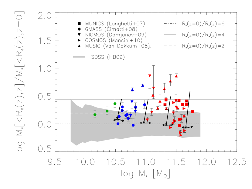
Figure 4.— Ratio between the projected stellar mass within the estimated half-mass radius $R_{e}$ for passively evolving ETG progenitors at $z\gtrsim 1$ and the average local value within the same physical radius and for the same overall stellar mass. The data points include observations of individual passively evolving galaxies with spectroscopic redshifts $z\gtrsim 1$ by Longhetti et al. (2007), Cimatti et al. (2008), Damjanov et al. (2009), Mancini et al. (2010), and van Dokkum et al. (2008). The shaded area shows the distribution of local SDSS galaxies (Hyde & Bernardi 2009). The thin lines illustrate the expected stellar mass ratio for different size increase from high$-z$ to the present, on adopting a local Sérsic index $n=4$ (see § 5.3 for more details). As in Fig. 2, thick lines with arrows illustrate typical evolutionary tracks of massive galaxies according to our reference model (with $f_{\sigma}=1.5$ and $z_{\rm form}=3$).

In Fig. 4 we plot the ratio between the projected mass of high redshift and local ETGs within the same physical radius, namely, the half-luminosity radius of high-redshift ETGs. In detail, since for high redshift ETGs $M_{\star}(<R_{e}(z),z)=M_{\star,\rm tot}/2$, the ratio comes to

$$\frac{M_{\star}(<R_{e}(z),z=0)}{M_{\star}(<R_{e}(z),z)}=2\,{\Gamma\left[2\,n,b_{n}\,\left({R_{e}(z)\over\langle R_{e}(z=0)\rangle}\right)^{1/n}\right]}~{},$$ (14)

where $\Gamma$ is the (normalized) incomplete Gamma function. Thus if the total mass does not change significantly, the quantity $M_{\star}(<R_{e}(z),z)/M_{\star}(<R_{e}(z),z=0)$ depends only on the ratio $r=R_{e}(z)/\langle R_{e}(z=0)\rangle$ and on the final Sérsic index $n$.

To plot the data points under the hypothesis of no mass evolution, we compute the ratio $r$ using the observed $R_{e}(z)$, and exploiting the observed stellar mass $M_{\star}$ to derive $\langle R_{e}(z=0)\rangle$ from the local $R_{e}-M_{\star}$ relation presented in Fig. 2. The horizontal lines has been computed for three values of $r$; for the sake of definiteness we adopt $n=4$. The thick lines with arrows illustrate the evolutionary track of massive galaxies according to our reference model with $f_{\sigma}=1.5$ and $z_{\rm form}=3$; these are found to be in encouraging agreement with the distribution of data points.

In the case of local ETGs we can define a ratio $r^{\prime}\equiv R_{e}(z=0)/\langle R_{e}(z=0)\rangle$ and compute the analogous of the mass ratio defined by Eq. (14). The shaded area, containing $65\%$ of local ETGs, illustrates the uncertainty of data points and of the horizontal lines associated to the assumption of an average half radius $\langle R_{e}(z=0)\rangle$.

Data points in Fig. 4 show that a significant fraction of high redshift passively evolving galaxies exhibit stellar mass inside their inferred half-mass radius larger by a factor $2-6$ than the mass of their local counterparts within the same physical radius.

Keeping mass and structural index $n=4$ constant, larger mass ratios can be obtained increasing the half luminosity radius by a factor from $2$ to $6$ (cf. horizontal lines). If we allow the structural index $n$ to vary by one, as suggested by the simulations of Naab et al. (2009), the change is minimal; even structural changes from $n=4$ to $n=8$ still would require a size increase by a factor of $\approx 6$ in order to explain galaxies with the largest mass ratio.

This result suggests that the mass inside this physical radius has on the average decreased and disfavors mechanisms that increase the size by only adding stars in the outer regions of the ETGs. We notice that our argument involves a significant fraction of the total galaxy mass. Contrariwise, the comparison of stellar surface density profiles within $R_{e}/50$ as performed by Hopkins et al. (2009a) refers only to a tiny fraction of the mass. It is interesting to note that Naab et al. (2009) find in their simulations that the dynamical friction is able to decrease the total mass inside $\lesssim 1$ kpc.

On the same line, massive ETGs with their large sizes, steeper correlation between effective radii and mass and large Sérsic index (Lauer et al. 2007b; Kormendy et al. 2009) clearly stand as representative cases of galaxies which experienced robust puffing up by quasar feedback. Moreover, the correlation of the central BH mass with Sérsic index $n$ (Graham et al. 2003; Graham & Driver 2007) for massive ETGs is consistent with the hypothesis that the strong feedback from the most massive BHs has led to a substantial increase of $n$.

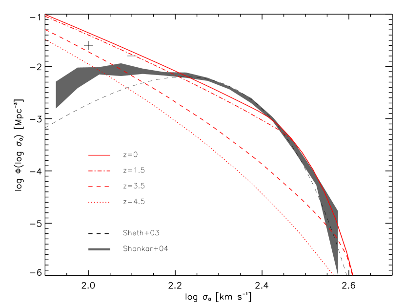
Figure 5.— Velocity distribution function. Our results at different redshifts are compared with the observational estimates of the local velocity distribution function by Sheth et al. (2003) and Shankar et al. (2004).

5.4. Velocity dispersion evolution

As mentioned in § 3, velocity dispersion has so far been determined only for a few individual high-$z$ spheroidal galaxies. The galaxy GMASS 2470 at $z\approx 1.4$ (Cappellari et al. 2009) and galaxy $\#$250425 at $z=1.82$ (Onodera et al. 2010) are already close to the local value for their mass, while $1255-0$ at $z\approx 2.2$ has a best fit velocity dispersion significantly higher than the most massive local galaxies. Thus in the two first cases evolution should have occurred before the cosmic time corresponding to the observed redshift, whereas significant evolution in size and velocity dispersion has to occur for the higher redshift galaxy. The studies of velocity dispersions by Cenarro & Trujillo (2009) and Cappellari et al. (2009), based on stacked spectra, suggest that velocity dispersion evolution is on the average needed.

An interesting hint on size and velocity dispersion average evolution can be derived by studying the velocity dispersion distribution (VDF) of local ETGs (Sheth et al. 2003), following the approach by Cirasuolo et al. (2005). From Eqs. (6) and (7), taking $n_{i}=3$ and $n_{f}=5$, we find, for the typical values of the parameters discusses above ($f_{\sigma}=1.5$, $r=4$), the relation $\sigma_{0,f}=0.6\,V_{\rm H}$; this associates to each forming halo the final velocity dispersion of the most massive hosted galaxy. By combining it with the formation rate of halos (see Appendix A) for redshifts $z\gtrsim 1$ we get the distribution function of the stellar velocity dispersions (VDF). From Fig. 5 it is apparent that the predicted VDF is in good agreement with the observational estimate by Sheth et al. (2003). We stress that the observed VDF highly constrains the global history of DM galaxy halos and of their stellar content, and therefore is an important benchmark for models of ETG formation (see also Loeb & Peebles 2003).

A change of the slope of the relationship between luminosity and velocity dispersion at low luminosity has been claimed by several authors (Shankar et al. 2006; Lauer et al. 2007a). In particular, Lauer et al. (2007a) show that the change in slope occurs at about the same luminosity $M_{V}\approx-21$, where the slope of the size vs. luminosity relation also changes (see § 6.2). Once more this feature occurs at the transition from supernova-dominated to quasar-dominated feedback regime.

An additional relevant aspect is related to the $M_{\bullet}$ vs. $\sigma_{0}$ and $M_{\bullet}$ vs. $M_{\star}$ correlations. The Granato et al. (2004) model, which we take as a reference, predicts that the mass in stars formed before the quasar shining is strictly related to the mass of the central BH, since the growth of the reservoir, which eventually furnishes the mass to the BH, is strictly proportional to the starforming activity (cf. Eq. [A20]). Marconi & Hunt (2003) and Häring & Rix (2004) pointed out that the $M_{\bullet}$ vs. $M_{\star}$ relation for ETGs and bulges exhibits a scatter comparable with that in the $M_{\bullet}$ vs. $\sigma_{0}$ relation.

In this context it is interesting to mention that, according to Lauer et al. (2007a), the extrapolation of the $\sigma_{0}$ vs. $M_{\bullet}$ relationship holding at low mass to higher mass galaxies would predict BH masses smaller than those inferred from the stellar mass. This is expected if the velocity dispersion decreased more significantly for higher mass galaxies, hosting more massive BHs and subject to stronger quasar feedback.

6. Summary and conclusions

The half-luminosity radius of high redshift passively evolving massive galaxies is observed to be on the average significantly smaller than that of their local counterparts with the same stellar mass, but in agreement with theoretical predictions based on the largely accepted assumption that most of the stars have been formed during dissipative collapse of cold gas. However, observations also show that the size distribution of high redshift ETG progenitors is broader than the corresponding distribution for local ETGs. While a significant fraction of massive high redshift ETGs already exhibit sizes as large as those of their local counterparts with the same mass, for a bunch of ETGs the size has to increase by a factor of $5-10$ to match the local half mass radius. Though still scanty, the available data on velocity dispersions are suggestive of a correspondingly large scatter of the ratios between high-$z$ and local values at fixed stellar mass.

The analysis of several data sets, discussed in § 2, and notably of the large sample by Maier et al. (2009) with spectroscopic redshifts, strongly suggests that most of the size evolution occurs at $z\gtrsim 1$, while at $z\lesssim 1$ sizes increase by no more than $40\%$. Moreover, a large fraction of high-$z$ passively evolving galaxies have projected stellar mass within their effective radii a factor of $2$ larger than those of local ETGs with the same stellar mass, within the same physical radius (see § 5.2).

All the above results are easily accounted for if most of the size evolution is due to a puffing up driven by the rapid expulsion of large amounts of mass, as proposed by Fan et al. (2008). That most of the baryons initially associated to the DM halo have to be expelled is strongly indicated by the fact that the baryon to DM mass ratio in galaxies is much smaller than the cosmic value. The quasar-driven winds advocated by Fan et al. (2008) occur in the most massive galaxies, while below $M_{\star}\approx 2\times 10^{10}\,M_{\odot}$ the dominant energy input into the interstellar medium comes from supernova explosions which induce a slower mass loss. The Fan et al. (2008) model therefore predicts a milder size evolution for the less massive spheroidal galaxies, while the size evolution of the more massive galaxies should parallel the quasar evolution, with a delay of about $0.5-1$ Gyr. The dichotomy between low- and high-mass galaxies, i.e., between supernova and quasar driven feedback, is mirrored in the increase of Sérsic index with stellar mass, in the flattening of the total mass vs. velocity dispersion relation toward massive galaxies, and in corresponding steepening of the correlation between effective radii and stellar mass.

The alternative explanation invoking minor mergers faces a couple of difficulties (see also Nipoti et al. 2009a,b). The analysis of the mass function evolution shows that, under the hypothesis of pure mass evolution, the upper limits to the mass increase are a factor $\approx 2$ and a factor $\approx 1.7$ since $z\approx 2$ and $z\approx 1.5$, respectively. Also the increase is expected to be gradual and rather uniform, so that practically all galaxies undergo the same mass increase. As a consequence almost all high redshift massive ETGs must evolve by a factor $\lesssim 2.2-3$. While this upper limit may be consistent with the average evolution of the size, the model does not account for the substantially broader size distribution, for given stellar mass, at high, compared to low, redshifts. In particular, since dry minor mergers require a long timescale $\approx 10$ Gyr to produce their full effects, they can not not explain why a significant fraction of the high-$z$ ETGs are already on the local mass-size relationship. Moreover, the upper limit in mass entails a factor of $\lesssim 3$ in size evolution since $z\approx 2$, while at the same redshift there are ETGs with half mass undersized by a factor $6-10$. On the positive side, for the minor merger scenario, the simulations by Naab et al. (2009) show that dynamical friction is able to remove part of the mass from the central regions in line with what suggested by observations (see Fig. 4).

The virial theorem tells us that the velocity dispersion scales as $\sigma^{2}\propto S_{D}\,M/r$, where $S_{D}$ is a structure factor defined by Prugniel & Simien (1997) in the case of a Sérsic profile. Since the rapid loss of a large mass fraction destabilizes the mass distribution, it may be expected that the final equilibrium configuration differs from the initial one. In fact, the data by van Dokkum et al. (2010) and simulations indicate that the Sérsic index of local galaxies is, on average, higher than for high-$z$ galaxies. If so, the variation of $S_{D}$ partially compensates the effect on $\sigma$ of the size increase. Although measurements of the kinematic properties of high-$z$ galaxies are scarce, a velocity dispersion evolution compatible with the expansion scenario is indicated (see § 5.4).

Appendix A Overview of our reference model

In recent years we developed a model of galaxy formation with focus on the evolution of baryons within protogalactic spheroids. Baryons have been followed through simple physical recipes emphasizing the effects of the collapse and cooling and of the energy fed back to the intragalactic gas by supernova (SN) explosions and by accretion onto the nuclear supermassive black holes (BHs; see Granato et al. 2001, 2004; Lapi et al. 2006, 2008; Mao et al. 2007; Fan et al. 2008). The main motivation was to enlighten the relevant physical processes shaping galaxy formation, to keep calculations easily reproducible and to suggest which processes should be implemented in the much more complex and much less reproducible numerical simulations.

The model transparently shows how physical processes acting on the baryons speeds up the formation of more massive galaxies. As a result, although the DM assembly follows a bottom-up hierarchy, galaxies and their active nuclei evolve in a way that appears opposite to the hierarchy in DM, following a pattern that we named Antihierarchical Baryon Collapse (ABC). We notice that it fully corresponds from the observational point of view to the so called downsizing.

We defer the interested reader to the above papers for a full account of the physical justification and a detailed description of the model, with appropriate acknowledgment of previous work. Here we present a short summary of its main features, and provide useful analytic approximations for quantities of relevance in this context.

A.1. DM sector

As for the treatment of the DM in galaxies, the model follows the standard hierarchical clustering framework, and takes into account the outcomes of recent intensive high-resolution $N-$body simulations of halo formation in a cosmological context (see Zhao et al. 2003; Diemand et al. 2007; Hoffmann et al. 2007; Ascasibar & Gottloeber 2008). In these studies, two distinct phases in the growth of DM halos have been recognized: an early fast collapse, and a later slow accretion phase. During the early collapse, a substantial mass is gathered through major mergers, which effectively reconfigure the gravitational potential wells and cause the collisionless DM particles to undergo dynamical relaxation and isotropization (Lapi & Cavaliere 2009). During the later phase, moderate amounts of mass, around $20-50\%$, are slowly accreted mainly onto the halo outskirts, little affecting the inner structure and potential, but quiescently rescaling upward the overall halo size. From the baryon point of view, the early phase — our main interest here — supports the dissipationless collapse of baryons to originate a spheroidal structure dominated by random motions (see also Cook et al. 2009).

Halos harboring a massive elliptical galaxy once created, even at high redshift, are rarely destroyed, while at low redshifts they are possibly incorporated within galaxy groups and clusters. Thus at $z\gtrsim 1$, the halo formation rate can be reasonably well approximated by the positive term in the derivative of the halo mass function with respect to cosmic time (e.g., Haehnelt & Rees 1993; Sasaki 1994). The halo mass function derived from numerical simulations (e.g., Jenkins et al. 2001) is well fit by the Sheth & Tormen (1999, 2002) formula, that improves over the original Press & Schechter (1974) expression (well known to under-predict by a large factor the massive halo abundance at high redshift). Adopting the Sheth & Tormen (1999) mass function $N_{\mathrm{ST}}(M_{\rm H},t)$, the formation rate of DM halos is given by

$${\mathrm{d}^{2}\,N_{\mathrm{ST}}\over\mathrm{d}M_{\rm H}\,\mathrm{d}t}=\left[{a\,\delta_{c}(t)\over\sigma^{2}(M_{\rm H})}+{2\,p\over\delta_{c}(t)}\,{\sigma^{2\,p}(M_{\rm H})\over\sigma^{2\,p}(M_{\rm H})+a^{p}\,\delta_{c}^{2\,p}(t)}\right]\,\left|{\mathrm{d}\delta_{c}\over\mathrm{d}t}\right|\,N_{\mathrm{ST}}(M_{\rm H},t)~{};$$ (A1)

here $a=0.707$ and $p=0.3$ are constants obtained by comparison with $N$-body simulations, $\sigma(M_{\rm H})$ is the mass variance of the primordial perturbation field computed from the Bardeen et al. (1986) power spectrum with correction for baryons (Sugiyama 1995) and normalized to $\sigma_{8}\approx 0.8$ on a scale of $8\,h^{-1}$ Mpc, and $\delta_{c}(t)$ is the critical threshold for collapse extrapolated from the linear perturbation theory.

As for the density distribution of DM halos we adopt as a reference the profile proposed by Navarro et al. (1997) and characterized by a scale radius $r_{s}$ and by the ratio of the virial to the scale radius $c=R_{\rm H}/r_{s}$, the concentration parameter, with typical values around $4$ at halo formation (e.g., Zhao et al. 2003). The halo circular velocity $V_{\rm H}=(G\,M_{\rm H}/R_{\rm H})^{1/2}$ characterizes the DM potential well; the associated velocity dispersion is $\sigma_{\rm DM}=f(c)^{1/2}\,V_{\rm H}$, where $f(c)\approx 2/3+(c/21.5)^{0.7}$ is a weak function of the concentration parameter of order $1$ (see Mo et al. 1998).

A.2. Baryonic sector

During the fast collapse phase, a rapid sequence of major mergers build up a DM halo of mass $M_{\rm H}$. At that time a mass $M_{\rm inf}=f_{b}\,M_{\rm H}$ of baryonic matter, in cosmic proportion $f_{b}\approx 0.2$ with the DM, is shock heated to the virial temperature by falling into the forming DM gravitational potential well. This hot gas cools and flows toward the central region at a rate

$$\dot{M}_{\mathrm{cond}}={M_{\mathrm{inf}}\over t_{\mathrm{cond}}}$$ (A2)

over the condensation timescale $t_{\mathrm{cond}}=\max[t_{\mathrm{cool}}(R_{\rm H}),t_{\mathrm{dyn}}(R_{\rm H})]$, namely, the maximum between the dynamical and the cooling time at the halo virial radius $R_{\rm H}$. When computing the cooling time, a clumping factor in the gas $\mathcal{C}\gtrsim$ a few, as suggested by numerical simulations (e.g., Gnedin & Ostriker 1997; Iliev et al. 2006), implies $t_{\mathrm{cool}}(R_{\rm H})\lesssim t_{\mathrm{dyn}}(R_{\rm H})$ on relevant galaxy scales at $z\gtrsim 1$.

We recall that the star formation in galaxy halos is a quite inefficient process (see Fig. A1), since only a minor fraction $10-20\%$ of the available baryons are cycled through stars in more massive halos and the fraction is rapidly decreasing with decreasing halo mass. As a result, the present-day cosmic mass density in stars is only a few percent of the mass density in baryons (e.g., Shankar et al. 2006). Thus the formation of the most massive galaxy in a halo is a process that involves only a fraction smaller than $20-30\%$ of its original baryons and DM. It is natural to assume that the material is rapidly put together by a few major mergers in the central regions of the halo. In these mergers the angular momentum decays on a dynamical friction timescale $t_{\mathrm{DF}}\approx 0.2\,(\xi/\ln{\xi})\,t_{\mathrm{dyn}}$, where $\xi\equiv M_{\rm H}/M_{\rm c}$ holds in terms of typical cloud mass $M_{\rm c}$ involved in major mergers (e.g. Mo & Mao 2004); these are very frequent at high redshift and in the central regions of halos during the fast collapse phase of DM evolution, implying $\xi\sim$ a few and hence a short $t_{\mathrm{DF}}$. Thus the effects of angular momentum can be neglected.

The model also assumes that quasar (QSO) activity removes not only cold gas from the galaxy, but also hot gas from the halo through winds at a rate $\dot{M}_{\mathrm{inf}}^{QSO}$, to be quantitatively discussed next; the equation for the diffuse hot gas is then

$$\dot{M}_{\mathrm{inf}}=-\dot{M}_{\mathrm{cond}}-\dot{M}_{\mathrm{inf}}^{QSO}~{}.$$ (A3)

The cold gas piled up by the cooling of hot gas, is partially consumed by star formation ($\dot{M}_{\star}$), and partially removed to a warm/hot phase endowed with long cooling time by the energy feedback from SNae ($\dot{M}_{\mathrm{cold}}^{SN}$) and QSO activity ($\dot{M}_{\mathrm{cold}}^{QSO}$):

$$\dot{M}_{\mathrm{cold}}=\dot{M}_{\mathrm{cond}}-[1-\mathcal{R}(t)]\dot{M}_{\star}-\dot{M}_{\mathrm{cold}}^{SN}-\dot{M}_{\mathrm{cold}}^{QSO}~{},\\$$ (A4)

where $\mathcal{R}(t)$ is the fraction of gas restituted to the cold component by the evolved stars. It depends on time (particularly soon after the onset of star formation) and on the assumed initial mass function (IMF). We adopt for reference a pseudo-Chabrier IMF of shape $\phi(m_{\star})=m_{\star}^{-x}$ with $x=1.4$ for $0.1\leqslant m_{\star}\leqslant 1\,M_{\odot}$ and $x=2.35$ for $m_{\star}>1\,M_{\odot}$. The often used approximation of instantaneous recycling implies $\mathcal{R}\approx 0.54$ (for a Salpeter IMF one has $\mathcal{R}\approx 0.3$). The mass of cold baryons that is going to be accreted onto the central supermassive BH is small enough to be neglected in the above equation.

Stars are formed at a rate

$$\dot{M_{\star}}=\int\frac{\mathrm{d}M_{\mathrm{cold}}}{\max[t_{\mathrm{cool}},t_{\mathrm{dyn}}]}\approx\frac{M_{\mathrm{cold}}}{t_{\star}}~{},$$ (A5)

where now $t_{\mathrm{cool}}$ and $t_{\mathrm{dyn}}$ refer to a mass shell $\mathrm{d}M_{\mathrm{cold}}$, and $t_{\star}$ is the star formation timescale averaged over the mass distribution. Star formation promotes the gathering of some cool gas into a low-angular-momentum reservoir around the central supermassive BH. A viable mechanism for this process is the radiation drag (see discussion by Umemura 2001; Kawakatu & Umemura 2002; Kawakatu et al. 2003), which has the nice feature of predicting a mass transfer rate to the reservoir proportional to the SFR:

$$\dot{M}_{\rm inflow}\approx\frac{L_{\star}}{c^{2}}\,\left(1-e^{-\tau_{\rm RD}}\right)\approx\alpha_{\rm RD}\times 10^{-3}\,\dot{M}_{\star}\,\left(1-e^{-\tau_{\rm RD}}\right)~{};$$ (A6)

the constant of proportionality $\alpha_{\rm RD}\sim 1-3$ can be fixed to produce a good match to the correlation between the spheroid and the supermassive BH masses observed in the local Universe, while the quantity

$$\tau_{\rm RD}(t)=\tau_{\rm RD}^{0}\,{Z(t)\over Z_{\odot}}\,{M_{\rm cold}(t)\over 10^{12}\,M_{\odot}}\,\left({M_{\rm H}\over 10^{13}\,M_{\odot}}\right)^{-2/3}~{}$$ (A7)

represents the effective optical depth of the gas clouds in terms of the normalization parameter $\tau_{\rm RD}^{0}\sim 1-2$ (for more details, see the discussion around Eqs. [14] to [17] in Granato et al. 2004).

Eventually, the gas stored in the reservoir accretes on to the BH powering the nuclear activity; usually, plenty of material is supplied to the BH, so that the latter can accrete close to the Eddington limit

$$\dot{M}_{\bullet}=\lambda_{\rm Edd}\,{1-\epsilon\over\epsilon}\,{M_{\bullet}\over t_{\rm Edd}}$$ (A8)

and grows almost exponentially from a seed of $10^{2}\,M_{\odot}$; the $e-$folding time involves the Eddington timescale $t_{\rm Edd}\approx 4\times 10^{8}$ yr, the radiative efficiency $\epsilon\approx 0.1$, and the actual Eddington ratio $\lambda_{\rm Edd}\sim 0.3-3$. The reservoir mass variation is ruled by the balance between the inflow due to radiation drag and the accretion onto the BH

$$\dot{M}_{\rm res}=\dot{M}_{\rm inflow}-\dot{M}_{\bullet}~{},$$ (A9)

between the inflow due to radiation drag and the accretion onto the BH.

The energy fed back to the gas by SN explosions and BH activity regulates the ongoing star formation and BH growth. The two feedback processes have very different dependencies on halo mass and on galaxy age. The feedback due to SN explosions removes the starforming gas at a rate

$$\dot{M}_{\mathrm{cold}}^{SN}=\beta_{SN}\,\dot{M}_{\star}~{},$$ (A10)

where the efficiency of gas removal

$$\beta_{SN}=\frac{N_{SN}\,\epsilon_{SN}\,E_{SN}}{E_{\mathrm{bind}}}\approx 0.6\left(\frac{N_{SN}}{8\times 10^{-3}/M_{\odot}}\right)\left(\frac{\epsilon_{SN}}{0.05}\right)\left(\frac{E_{SN}}{10^{51}\mathrm{erg}}\right)\left(\frac{M_{\rm H}}{10^{12}M_{\odot}}\right)^{-2/3}\left(\frac{1+z}{4}\right)^{-1}$$ (A11)

depends on the number of SNae per unit solar mass of condensed stars $N_{SN}$ (of order $1.4\times 10^{-2}$ for the Chabrier IMF), on the energy per SN available to remove the cold gas $\epsilon_{SN}\,E_{SN}$, and on the specific binding energy of the gas within the DM halo, $E_{\mathrm{bind}}$. Following Zhao et al. (2003) and Mo & Mao (2004), the latter quantity has been estimated for $z\gtrsim 1$ as $E_{\mathrm{bind}}=V_{\mathrm{H}}^{2}\,f(c)\,(1+f_{\mathrm{b,i}})/2\approx 3.2\times 10^{14}\,(M_{\rm H}/10^{12}\,M_{\odot})^{2/3}\,[(1+z)/4]\,{\mathrm{cm}^{2}~{}\mathrm{s}^{-2}}$

In Granato et al. (2004) it is assumed that the QSO feedback acts both on the cold as well as on the infalling gas, unbinding them from the DM halo potential well at a rate $\dot{M}_{\rm inf,cold}^{\rm QSO}=\dot{M}_{\rm wind}\times M_{\rm inf,cold}/(M_{\rm inf}+M_{\rm cold})$ proportional to the corresponding mass fraction and to the wind mass outflow rate

$$\dot{M}_{\rm wind}=\frac{L_{QSO}}{E_{\rm bind}}~{},$$ (A12)

with

$$L_{QSO}\approx 2\times 10^{44}\,\epsilon_{QSO}\left(\frac{M_{\bullet}}{10^{8}\ M_{\odot}}\right)^{3/2}~{}\mathrm{erg~{}s}^{-1}~{}.$$ (A13)

Here $\epsilon_{QSO}=(f_{h}/0.5)\,(f_{c}/0.1)\,N_{23}$ is the strength of QSO feedback, expected to be close to unity; $f_{h}$ parameterizes the efficiency of energy transfer from winds generated close to the accretion disc to the general interstellar medium, $f_{c}$ is the covering factor of such winds and $N_{23}$ is the hydrogen column density toward the BH in units of $10^{23}$ cm^-2 (cf. Eqs. [29], [30] and [31] in Granato et al. 2004). With $\epsilon_{\rm QSO}\approx 1.3$ the bright end of the galaxy luminosity function is reproduced (Lapi et al. 2006).

As a consequence, the QSO feedback grows exponentially during the early phases of galaxy evolution, following the exponential growth of the supermassive BH mass. It is is negligible in the first $0.5$ Gyr in all halos, but abruptly becomes dominant in DM halos more massive than $10^{12}\,M_{\odot}$. Eventually, in these systems most of the gas becomes unbound from the potential well of the galaxy halo, so that star formation and BH activity itself come to an end on a timescale which is shorter for more massive galaxies.

Indeed, the positive feedback on BH growth caused by star formation, in cooperation with the immediate and negative feedback of SN, and the abrupt and dramatic effect of QSO feedback, are able to reverse the formation sequence of the baryonic component of galaxies compared to that of DM halos: the star formation and the buildup of central BHs are completed more rapidly in the more massive halos, thus accounting for the phenomenon now commonly referred to as downsizing.

The model yields as outputs the time evolutions of stars and gas (including metals) components of the galaxies and of the associated active galactic nuclei. When the star formation, gas abundance and the chemical evolution history of a galaxy within a DM halo of given mass have been computed, the dust abundance can be inferred (e.g., Mao et al. 2007). Then the spectral energy distribution as a function of time from extreme-UV to radio frequencies can be obtained through spectrophotometric codes, such as GRASIL, which includes a tretment of dust reprocessing (Silva et al. 1998; Schurer et al. 2009). Coupling these results with the DM halo formation rate, we can obtain the statistics of galaxies and supermassive BHs/QSOs as a function of cosmic time, in different observational bands.

A.3. Analytic approximations

By analyzing the results of the numerical solution for the full set of equations given above, it is apparent that in massive galaxies the term of QSO feedback is important only during the final stage of BH growth, around $2-3$ $e-$folding times (approximately $10^{8}$ yr) before the peak of QSO luminosity, when the energy discharged by the QSO is so powerful to unbind most of the residual gas, quenching both star formation and further accretion onto the supermassive BH. On the other hand, in less massive galaxies the central BH mass and the associated accretion is not able to stop star formation, which lasts for several Gyrs. The duration of the star formation $\Delta t_{\mathrm{burst}}$ can be approximated by a simple analytical form

$$\Delta t_{\mathrm{burst}}\approx 6\times 10^{8}\,\left(\frac{1+z}{4}\right)^{-1.5}\,\mathcal{F}\left(\frac{M_{\rm H}}{10^{12}\,M_{\odot}}\right)~{}~{}\mathrm{yr}~{},$$ (A14)

where $\mathcal{F}(x)=1$ for $x\gtrsim 1$ and $\mathcal{F}(x)=x^{-1}$ for $x\lesssim 1$. A good approximation for the star formation history in massive galaxies is obtained by neglecting the QSO feedback effect in Eqs. (A3) and (A4) and by abruptly stopping star formation and accretion onto the central BH after $\Delta t_{\mathrm{burst}}$ since halo formation.

Then Eqs. (A3) and (A4) can be easily solved, with the outcome that the infalling mass declines exponentially as

$$M_{\mathrm{inf}}(t)=M_{\rm b,i}\,\mathrm{e}^{-t/t_{\mathrm{cond}}}~{},$$ (A15)

where we assume $M_{\rm b,i}=f_{b}\,M_{\rm H}$, with $f_{b}=\Omega_{b}/\Omega_{\rm DM}\approx 0.2$. The cold gas mass evolves according to

$$M_{\mathrm{cold}}(t)=\frac{f_{b}M_{\rm H}}{s\gamma-1}\,\left[\mathrm{e}^{-t/t_{\mathrm{cond}}}-\mathrm{e}^{-s\,\gamma\,t/t_{\mathrm{cond}}}\right]~{};$$ (A16)

here we have introduces the shorthand $\gamma\equiv 1-\mathcal{R}+\beta_{\rm SN}$. The quantity $s\equiv t_{\mathrm{cond}}/t_{\mathrm{\star}}$ is the ratio between the timescale for the large-scale infall estimated at the virial radius and the star formation timescale in the central region; it corresponds to $s\approx 5$, both for an isothermal or NFW density profile with standard value of the concentration parameter $c\approx 4$ at halo formation. We notice that the dependence on the fraction of gas restituted by the stars is quite weak and that the value obtained by the hypothesis of instantaneous recycling can be used.

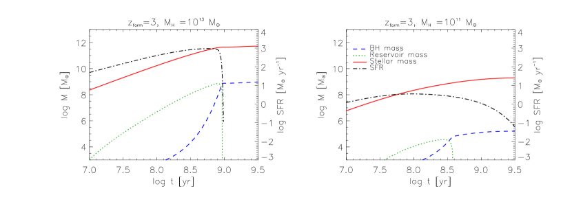
Figure 6.— Evolution with galactic age of the stellar, reservoir, BH masses (left axis scale) and of the SFR (right axis scale) in our reference model (Granato et al. 2004) for galaxy halos with mass $10^{13}\,M_{\odot}$ and $10^{11}\,M_{\odot}$ formed at $z_{\rm form}=3$.

The corresponding stellar mass reads:

$$M_{\star}(t)=\frac{s\,f_{b}M_{\rm H}}{s\gamma-1}\,\left[1-\mathrm{e}^{-t/t_{\mathrm{cond}}}-{1\over s\gamma}\,\left(1-\mathrm{e}^{-s\,\gamma\,t/t_{\mathrm{cond}}}\right)\right]~{};$$ (A17)

the mass of all stars formed during the main episode of star formation is then $M_{\star}^{\rm f}\approx M_{\star}(\Delta t_{\mathrm{burst}})$.

In Eqs. (A13), (A14), and (A16) the condensation timescale is well approximated by

$$t_{\mathrm{cond}}\approx 9\times 10^{8}\,\left(\frac{1+z}{4}\right)^{-1.5}\,\left(\frac{M_{\rm H}}{10^{12}\,M_{\odot}}\right)^{0.2}~{}~{}\mathrm{yr}~{}.$$ (A18)

The scaling with redshift and mass mainly reflects the behavior of the dynamical/cooling time, while a mild dependence on $M_{\rm H}$ is also related to the impact of the energy feedback from the QSO on the infalling gas, which is stronger for more massive halos hosting more massive BH.

A good approximation for $f_{\rm gas}$, i.e. the ratio between the stellar and gaseous mass immediately before the gas is swept away by the QSO feedback, can be obtained using Eqs. (A16) and (A17). The gas mass includes both the cold gas and the gas restituted by the stars. The latter is estimated as $\mathcal{R}\,M_{\star}$ with $\mathcal{R}=0.3$, which corresponds to the gas returned by the stars about $0.1$ Gyr after a burst of star formation with a Chabrier’s IMF. We find that the results are well approximated by $f_{\rm gas}\approx(M_{\star}/10^{11}\,M_{\odot})^{0.2}$.

For $M_{\rm H}\gtrsim 3\times 10^{11}\,M_{\odot}$, corresponding to $M_{\star}\gtrsim 10^{10}\,M_{\odot}$, the dependence on halo mass and formation redshift of ratio $m$ between the halo mass and the surviving stellar mass (i.e. the present day stellar mass fraction) can be approximated as $m\approx 25\,(M_{\rm H}/10^{12}\,M_{\odot})^{0.1}\,[(1+z_{\rm form})/4]^{-0.25}$. At lower masses $m$ increases rapidly with decreasing $M_{\star}$ (see Shankar et al. 2006).

Finally, considering that all the mass flowed into the reservoir is eventually accreted by the BH and neglecting the mass of the seed BH ($M_{\bullet}^{0}\approx 10^{2}\,M_{\odot}$), one can write the relic BH mass as function of the overall mass in stars formed during the star forming phase $\Delta t_{\rm burst}$ as

$$M_{\bullet}^{\rm f}\approx\alpha_{\rm RD}\times 10^{-3}\,M_{\star}^{\rm f}\,(1-{\rm e}^{-\langle\tau_{\rm RD}\rangle})~{}.$$ (A19)

The time average of the optical depth $\langle\tau_{\rm RD}\rangle$ can be approximated as

$$\langle\tau_{\rm RD}\rangle\approx\tau_{\rm RD}^{0}\,\left(M_{\rm H}\over 10^{13}\,M_{\odot}\right)^{2/3}\,\left(1+z\over 4\right),$$ (A20)

implying $1-{\rm e}^{-\langle\tau_{\rm RD}\rangle}\approx 1$ for massive galaxies and $1-{\rm e}^{-\langle\tau_{\rm RD}\rangle}\approx\langle\tau_{\rm RD}\rangle\propto M_{\rm H}^{2/3}$ for less massive galaxies. As expected, most of the mass flows from the reservoir to the central BH in the final couple of $e-$folding times. At early times the ratio of the BH to the stellar mass is predicted to be much lower than the final value (cf. Fig. A1).

In Fig. A1 we show, as illustrative examples, the evolutions with galaxy age of the stellar, reservoir and BH masses, and of the star formation rate (SFR) for galaxies with halo masses of $10^{13}\,M_{\odot}$ and $10^{11}\,M_{\odot}$, formed at $z_{\rm form}=3$.

References

- (1)
- (2) Annibali, F., et al. 2007, A&A, 463, 455
- (3)
- (4) Ascasibar, Y., & Gottlöber, S. 2008, MNRAS, 386, 2022
- (5)
- (6) Bardeen, J.M., Bond, J.R., Kaiser, N., & Szalay, A.S. 1986, ApJ, 304, 15
- (7)
- (8) Bastian, N., & Goodwin, S.P. 2006, MNRAS, 369, L9
- (9)
- (10) Baumgardt, H., & Kroupa, P. 2007, MNRAS, 380, 1589
- (11)
- (12) Bell, E.F., McIntosh, D.H., Katz, N., & Weinberg, M.D. 2003, ApJS, 149, 289
- (13)
- (14) Bernardi, M., et al. 2010, MNRAS, in press (preprint arXiv0910.1093)
- (15)
- (16) Bernardi, M. 2009, MNRAS, 395, 1491
- (17)
- (18) Bernardi, M., et al. 2008, MNRAS, 391, 1191
- (19)
- (20) Bernardi, M., et al. 2007, AJ, 133, 1741
- (21)
- (22) Bernardi, M., et al. 2005, AJ, 129, 61
- (23)
- (24) Bezanson, R., et al. 2009, ApJ, 697, 1290
- (25)
- (26) Biermann, P., & Shapiro, S.L. 1979, ApJ, 230, L33
- (27)
- (28) Boily, C.M., & Kroupa, P. 2003, MNRAS, 338, 673
- (29)
- (30) Boylan-Kolchin, M., Ma, C.-P., & Quataert, E. 2006, MNRAS, 369, 1081
- (31)
- (32) Boylan-Kolchin, M., Ma, C.-P., & Quataert, E. 2008, MNRAS, 383, 93
- (33)
- (34) Borriello, A., Salucci, P., & Danese, L. 2003, MNRAS, 341, 1109
- (35)
- (36) Bouché, N., et al. 2007, ApJ, 671, 303
- (37)
- (38) Bower, R.G., Lucey, J.R., & Ellis, R.S. 1992a, MNRAS, 254, 589
- (39)
- (40) Bower, R.G., Lucey, J.R., & Ellis, R.S. 1992b, MNRAS, 254, 601
- (41)
- (42) Buitrago, F., et al. 2008, ApJ, 687, L61
- (43)
- (44) Caon, N., Capaccioli, M., & D’Onofrio, M. 1993, MNRAS, 265, 1013
- (45)
- (46) Cappellari, M., et al. 2006, MNRAS, 366, 1126
- (47)
- (48) Cappellari, M., et al. 2009, ApJ, 704, L34
- (49)
- (50) Cenarro, A.J., & Trujillo, I. 2009, ApJ, 696, L43
- (51)
- (52) Chabrier, G. 2003, PASP, 115, 763
- (53)
- (54) Cimatti, A., et al. 2008, A&Ap, 482, 21
- (55)
- (56) Cirasuolo, M., et al. 2010, MNRAS, 401, 1166
- (57)
- (58) Cirasuolo, M., et al. 2005, ApJ, 629, 816
- (59)
- (60) Cole, S., et al. 2001, MNRAS, 326, 255
- (61)
- (62) Collins, C.A., et al. 2009, Nature, 458, 603
- (63)
- (64) Cook, M., Lapi, A., & Granato, G.L. 2009, MNRAS, 397, 534
- (65)
- (66) Coppin, K., et al. 2006, MNRAS, 372, 1621
- (67)
- (68) Cowie, L.L., Songaila, A., Hu, E.M., & Cohen, J.G. 1996, AJ, 112, 839
- (69)
- (70) Cresci, G., et al. 2009, ApJ, 697, 115
- (71)
- (72) Croton, D.J., et al. 2006, MNRAS, 365, 11
- (73)
- (74) Daddi, E., et al. 2009, ApJ, 695, L176
- (75)
- (76) Damjanov, I., et al. 2009, ApJ, 695, 101
- (77)
- (78) de Vaucouleurs, G. 1953, MNRAS, 113, 134
- (79)
- (80) Diemand, J., Kuhlen, M., & Madau, P. 2007, ApJ, 667, 859
- (81)
- (82) Djorgovski, S., & Davis, M. 1987, ApJ, 313, 59
- (83)
- (84) D’Odorico, V., et al. 2004, MNRAS, 351, 976
- (85)
- (86) Dressler, A., et al. 1987, ApJ, 313, 42
- (87)
- (88) Drory, N., et al. 2005, ApJ, 619, L131
- (89)
- (90) Dye, S., et al. 2008, MNRAS, 386, 1107
- (91)
- (92) Fan, L., Lapi, A., De Zotti, G., & Danese, L. 2008, ApJ, 689, L101
- (93)
- (94) Faber, S.M., & Jackson, R.E. 1976, ApJ, 204, 668
- (95)
- (96) Fechner, C., & Richter, P. 2009, A&Ap, 496, 31
- (97)
- (98) Ferguson, H.C., et al. 2004, ApJ, 600, L107
- (99)
- (100) Ferrarese, L., & Ford, H. 2005, Space Science Reviews, 116, 523
- (101)
- (102) Ferreras, I., et al. 2009, MNRAS, 396, 1573
- (103)
- (104) Fontana, A., et al. 2006, A&Ap, 459, 745
- (105)
- (106) Fukugita M., et al., 2007, AJ, 134, 579
- (107)
- (108) Gallazzi, A., Charlot, S., Brinchmann, J., & White, S.D.M. 2006, MNRAS, 370, 1106
- (109)
- (110) Geyer, M.P., & Burkert, A. 2001, MNRAS, 323, 988
- (111)
- (112) Gnedin, N.Y., & Ostriker, J.P. 1997, ApJ, 486, 581
- (113)
- (114) Goodwin, S.P., & Bastian, N. 2006, MNRAS, 373, 752
- (115)
- (116) Graham, A.W., & Driver, S.P. 2007, ApJ, 655, 77
- (117)
- (118) Graham, A.W., Erwin, P., Trujillo, I., & Asensio Ramos, A. 2003, AJ, 125, 2951
- (119)
- (120) Granato, G.L., et al. 2004, ApJ, 600, 580
- (121)
- (122) Granato, G.L., et al. 2001, MNRAS, 324, 757
- (123)
- (124) Guo, Q., & White, S.D.M. 2009, MNRAS, 396, 39
- (125)
- (126) Haehnelt, M.G., & Rees, M.J. 1993, MNRAS, 263, 168
- (127)
- (128) Häring, N., & Rix, H.-W. 2004, ApJ, 604, L89
- (129)
- (130) Hills, J.G. 1980, ApJ, 235, 986
- (131)
- (132) Hoffman, Y., Romano-Díaz, E., Shlosman, I., & Heller, C. 2007, ApJ, 671, 1108
- (133)
- (134) Hopkins, P.F., et al. 2010, MNRAS, 401, 1099
- (135)
- (136) Hopkins, P.F., et al. 2009a, MNRAS, 398, 898
- (137)
- (138) Hopkins, P.F., et al. 2009b, ApJ, 691, 1424
- (139)
- (140) Hyde, J.B., & Bernardi, M. 2009, MNRAS, 394, 1978
- (141)
- (142) Iliev, I.T., et al. 2006, MNRAS, 369, 1625
- (143)
- (144) Jenkins, A., et al. 2001, MNRAS, 321, 372
- (145)
- (146) Jenkins, A., et al. 2001, MNRAS, 321, 372
- (147)
- (148) Johansson, P.H., Naab, T., & Burkert, A. 2009, ApJ, 690, 802
- (149)
- (150) Joung, M.R., Cen, R., & Bryan, G.L. 2009, ApJ, 692, L1
- (151)
- (152) Jørgensen, I., Franx, M., & Kjaergaard, P. 1993, ApJ, 411, 34
- (153)
- (154) Kajisawa, M., et al. 2009, ApJ, 702, 1393
- (155)
- (156) Kawakatu, N., & Umemura, M. 2002, MNRAS, 329, 572
- (157)
- (158) Kawakatu, N., Umemura, M., & Mori, M. 2003, ApJ, 583, 85
- (159)
- (160) Komatsu, E., et al. 2009, ApJs, 180, 330
- (161)
- (162) Kormendy, J., Fisher, D.B., Cornell, M.E., & Bender, R. 2009, ApJS, 182, 216
- (163)
- (164) Kriek, M., et al. 2009, ApJ, 700, 221
- (165)
- (166) Kroupa, P. 2001, MNRAS, 322, 231
- (167)
- (168) Lapi, A., & Cavaliere, A. 2009, ApJ, 692, 174
- (169)
- (170) Lapi, A., et al. 2008, MNRAS, 386, 608
- (171)
- (172) Lapi, A., et al. 2006, ApJ, 650, 42
- (173)
- (174) Lapi, A., Cavaliere, A., & Menci, N. 2005, ApJ, 619, 60
- (175)
- (176) Larson, R.B. 1974a, MNRAS, 166, 585
- (177)
- (178) Larson, R.B. 1974b, MNRAS, 169, 229
- (179)
- (180) Lauer, T.R., et al. 2007a, ApJ, 662, 808
- (181)
- (182) Lauer, T.R., et al. 2007b, ApJ, 664, 226
- (183)
- (184) Law, D.R., et al. 2009, ApJ, 697, 2057
- (185)
- (186) Lípari, S., et al. 2009, MNRAS, 398, 658
- (187)
- (188) Loeb, A., & Peebles, P.J.E. 2003, ApJ, 589, 29
- (189)
- (190) Longhetti, M., et al. 2007, MNRAS, 374, 614
- (191)
- (192) Magorrian, J., et al. 1998, AJ, 115, 2285
- (193)
- (194) Maier, C., et al. 2009, ApJ, 694, 1099
- (195)
- (196) Maller, A.H., et al. 2006, ApJ, 647, 763
- (197)
- (198) Mancini, C., et al. 2010, MNRAS, 401, 933
- (199)
- (200) Mandelbaum, R., et al. 2006, MNRAS, 368, 715
- (201)
- (202) Mao, J., et al. 2007, ApJ, 667, 655
- (203)
- (204) Marchesini, D., et al. 2009, ApJ, 701, 1765
- (205)
- (206) Marconi, A., & Hunt, L.K. 2003, ApJ, 589, L21
- (207)
- (208) McIntosh, D.H., et al. 2005, ApJ, 632, 191
- (209)
- (210) Mo, H.J., & Mao, S. 2004, MNRAS, 353, 829
- (211)
- (212) Mo, H.J., Mao, S., & White, S.D.M. 1998, MNRAS, 295, 319
- (213)
- (214) Moster, B.P., et al. 2010, 710, 903
- (215)
- (216) Naab, T., Johansson, P.H., Ostriker, J.P., & Efstathiou, G. 2007, ApJ, 658, 710
- (217)
- (218) Naab, T., Johansson, P.H., & Ostriker, J.P. 2009, ApJ, 699, L178
- (219)
- (220) Navarro, J.F., Frenk, C.S., & White, S.D.M. 1997, ApJ, 490, 493
- (221)
- (222) Nipoti, C., Londrillo, P., & Ciotti, L. 2003, MNRAS, 342, 501
- (223)
- (224) Nipoti, C., et al. 2009a, ApJ, 706, L86
- (225)
- (226) Nipoti, C., Treu, T., & Bolton, A.S. 2009b, ApJ, 703, 1531
- (227)
- (228) Onodera, M. et al. 2010, ApJL, in press (preprint arXiv:1004.2120)
- (229)
- (230) O’Sullivan, E., & Ponman, T.J. 2004, MNRAS, 349, 535
- (231)
- (232) Pérez-González, P.G., et al. 2008, ApJ, 675, 234
- (233)
- (234) Pozzetti, L., et al. 2007, A&Ap, 474, 443
- (235)
- (236) Press, W.H., & Schechter, P. 1974, ApJ, 187, 425
- (237)
- (238) Prochaska, J.X., & Hennawi, J.F. 2009, ApJ, 690, 1558
- (239)
- (240) Prugniel, P., & Simien, F. 1997, A&Ap, 321, 111
- (241)
- (242) Renzini, A. 2006, ARA&A, 44, 141
- (243)
- (244) Richstone, D.O., & Potter, M.D. 1982, ApJ, 254, 451
- (245)
- (246) Sandage, A., & Visvanathan, N. 1978, ApJ, 223, 707
- (247)
- (248) Sasaki, S. 1994, PASJ, 46, 427
- (249)
- (250) Schurer, A., et al. 2009, MNRAS, 394, 2001
- (251)
- (252) Serjeant, S., et al. 2008, MNRAS, 386, 1907
- (253)
- (254) Sérsic, J.L. 1963, Boletin de la Asociacion Argentina de Astronomia, 6, 41
- (255)
- (256) Shankar, F., et al. 2006, ApJ, 643, 14
- (257)
- (258) Shen, S., et al. 2003, MNRAS, 343, 978
- (259)
- (260) Sheth, R.K., & Tormen, G. 1999, MNRAS, 308, 119
- (261)
- (262) Sheth, R.K., & Tormen, G. 2002, MNRAS, 329, 61
- (263)
- (264) Sheth, R.K., et al. 2003, ApJ, 594, 225
- (265)
- (266) Sijacki, D., Springel, V., Di Matteo, T., & Hernquist, L. 2007, MNRAS, 380, 877
- (267)
- (268) Silk, J., & Rees, M.J. 1998, A&A, 331, L1
- (269)
- (270) Silva, L., et al. 2005, MNRAS, 357, 1295
- (271)
- (272) Silva, L., Granato, G.L., Bressan, A., & Danese, L. 1998, ApJ, 509, 103
- (273)
- (274) Simcoe, R.A., Sargent, W.L.W., Rauch, M., & Becker, G. 2006, ApJ, 637, 648
- (275)
- (276) Somerville, R.S., et al. 2008, MNRAS, 391, 481
- (277)
- (278) Springel, V., Di Matteo, T., & Hernquist, L. 2005, MNRAS, 361, 776
- (279)
- (280) Sugiyama, N. 1995, ApJs, 100, 281
- (281)
- (282) Stewart, K.R., et al. 2008, ApJ, 683, 597
- (283)
- (284) Szomoru, D., et al. 2010, ApJ, 714, L244
- (285)
- (286) Tacconi, L.J., et al. 2008, ApJ, 680, 246
- (287)
- (288) Tacconi, L.J., et al. 2010, Nature, 463, 781
- (289)
- (290) Thomas, D., Greggio, L., & Bender, R. 1999, MNRAS, 302, 537
- (291)
- (292) Toft, S., et al. 2007, ApJ, 671, 285
- (293)
- (294) Toft, S., et al. 2009, ApJ, 705, 255
- (295)
- (296) Tortora, C., et al. 2009, MNRAS, 396, 1132
- (297)
- (298) Trujillo, I., et al. 2004, ApJ, 604, 521
- (299)
- (300) Trujillo, I., et al. 2007, MNRAS, 382, 109
- (301)
- (302) Trujillo, I., et al. 2009, ApJ, 692, L118
- (303)
- (304) Umemura, M. 2001, ApJ, 560, L29
- (305)
- (306) Vale, A., & Ostriker, J.P. 2004, MNRAS, 353, 189
- (307)
- (308) Valentinuzzi, T., et al. 2010, ApJ, 712, 226
- (309)
- (310) van der Wel, A., et al. 2009, ApJ, 698, 1232
- (311)
- (312) van der Wel, A., et al. 2008, ApJ, 688, 48
- (313)
- (314) van Dokkum, P.G., et al. 2008, ApJ, 677, L5
- (315)
- (316) van Dokkum, P.G., Kriek, M., & Franx, M. 2009, Nature, 460, 717
- (317)
- (318) van Dokkum, P. G., et al. 2010, ApJ, 709, 1018
- (319)
- (320) Visvanathan, N., & Sandage, A. 1977, ApJ, 216, 214
- (321)
- (322) Wang, W.-H., Barger, A.J., & Cowie, L.L. 2009, ApJ, 690, 319
- (323)
- (324) White, S.D.M., & Rees, M.J. 1978, MNRAS, 183, 341
- (325)
- (326) Williams, R.J., et al. 2009, ApJ, 691, 1879
- (327)
- (328) Zhao, D.H., Mo, H.J., Jing, Y.P., Börner, G. 2003, MNRAS, 339, 12
- (329)
- (330) Zirm, A.W., et al. 2007, ApJ, 656, 66
- (331)