section[6mm]6mm0pc *subsection[6mm] , [  •  ][]

arXiv:1006.2174
TIFR/TH/10-15

        Abstract

The existence of a nontrivial interpolating function $h(\lambda)$ is one of the novel features of the new AdS₄/CFT₃ correspondence involving ABJM theory. At strong coupling, most of the investigation of semiclassical effects so far has been for strings in the $AdS_{4}$ sector. Several cutoff prescriptions have been proposed, leading to different predictions for the constant term in the expansion $h(\lambda)=\sqrt{\lambda/2}+c+\ldots$. We calculate quantum corrections for giant magnons, using the algebraic curve, and show by comparing to the dispersion relation that the same prescriptions lead to the same values of $c$ in this $CP^{3}$ sector. We then turn to finite-$J$ effects, where a comparison with the Lüscher F-term correction shows a mismatch for one of the three sum prescriptions. We also compute some dyonic and higher F-terms for future comparisons.

Contents

toc

1 Introduction

In the AdS/CFT correspondence [1, 2] between ABJM’s superconformal Chern–Simons-matter theory and IIA strings on $AdS_{4}\times CP^{3}$, the dispersion relation for a bound state of $Q$ magnons (or a dyonic giant magnon) is

$$E\equiv\Delta-\frac{J}{2}=\sqrt{\frac{Q^{2}}{4}+4h(\lambda)^{2}\sin^{2}\frac{p}{2}\>}.$$ (1)

One important difference from the $AdS_{5}\times S^{5}$ example is that $h(\lambda)$ is now a nontrivial function. It is related to the ’t Hooft coupling $\lambda$ as follows:

$$h(\lambda) =\sqrt{\dfrac{\lambda}{2}}+c+\mathcal{O}\Big{(}\frac{1}{\sqrt{\lambda}}\Big{)},\qquad\lambda\gg 1$$ (2)

$$h(\lambda)^{2} =\lambda^{2}+h_{4}\lambda^{4}+\mathcal{O}(\lambda^{6}),\qquad\>\lambda\ll 1.$$

The leading terms here come from the comparison with classical strings and with two-loop gauge-theory results [2, 6, 7, 8, 9, 10]. Both sides involve $\lambda$ via the AdS/CFT relation

$$\frac{R^{4}}{2^{5}\pi^{2}\alpha^{\prime 2}}=\lambda=\frac{N}{k}.$$ (3)

Four-loop gauge theory calculations [10, 11] show that $h_{4}=-4\zeta(2)\approx-6.58$. This rules out various simple interpolating functions one could imagine from the leading behaviours [8, 12].

The main goal of this paper is to calculate the value of $c$ from the one-loop corrections to the dispersion relation (1) of the giant magnon. The next subsection of the introduction reviews some previous calculations of $c$, which used a different classical solution. After that we discuss the cutoff prescriptions used, before turning to giant magnons in section 1.3.

1.1 The coefficient $c$ from spinning strings in AdS

A number of early ABJM papers studied spinning strings in an $AdS_{3}$ subspace. These have [13]

$$\Delta-S=f(\lambda)\log S$$ (4)

and at leading order $f(\lambda)=\sqrt{2\lambda}$ [2]. Two very different calculations of the one-loop, $o(1)$, semiclassical corrections were done:

• Several authors [14, 15, 16] found explicit modes using the worldsheet action, and obtained

  $$\delta E_{\mathrm{old}}=-5\frac{\log 2}{2\pi}\log S.$$

  Despite the classical solution being identical to those studied in $AdS_{5}\times S^{5}$, this quantum result is different to that of [17, 18, 19]. And the logic is that small fluctuations explore not only the $AdS_{3}$ subspace, but the other directions too.

• Using the proposed all-loop $sl(2)$ Bethe ansatz, [12] obtained

  $$\delta E_{\mathrm{BA}}=-3\frac{\log 2}{2\pi}\log S.$$

  Apart from trivial changes of constants, and one minus, the Bethe equations used for this $sl(2)$ sector are identical to those used in the $AdS_{5}\times S^{5}$ case [20, 21, 19].

Two ways to resolve this apparent discrepancy have been proposed. One is to notice that while the string calculation is an expansion in $1/\sqrt{\lambda}$, the Bethe ansatz calculation is a series in $1/h(\lambda)$. Expanding the latter in $1/\sqrt{\lambda}$ we can compare them:

$$f(\lambda) =2h(\lambda)-3\frac{\log 2}{2\pi}+\mathcal{O}\Big{(}\frac{1}{h}\Big{)}$$

$$=\sqrt{2\lambda}+\left(2c-3\frac{\log 2}{2\pi}\right)+\mathcal{O}\Big{(}\frac{1}{\sqrt{\lambda}}\Big{)}.$$

The order $\sqrt{\lambda}^{0}$ piece can be made to match the one-loop worldsheet result by setting [22]

$$c=-\frac{\log 2}{2\pi}.$$ (5)

The other way to resolve this is to modify the mode sum used. The simplest object from the worldsheet perspective, and that used by [14, 15, 16, 22], is

$$\delta E_{\mathrm{old}}\equiv\lim_{N\to\infty}\frac{1}{2}\sum_{n=-N}^{N}\omega_{n}$$

stopping at the same mode number $N$ for all modes. However, a different cutoff is more natural when computing these modes using the algebraic curve, namely to stop at a fixed radius $\left|x\right|$ in the spectral plane. This new prescription was shown by [20] to change the result of [14, 15, 16] to

$$\delta E_{\mathrm{new}}=-3\frac{\log 2}{2\pi}\log S$$

thus matching the Bethe ansatz calculation with $c=0$.

The fact that these two summation prescriptions (or regularisation schemes) give different results can perhaps be summarised by saying that these schemes refer to different coupling constants related by

$$\frac{1}{\sqrt{\lambda}}\;\to\;\frac{1}{\sqrt{\lambda}}\pm\frac{1}{\lambda}\left(\frac{\log 2}{2\pi}\right)$$

This is clearly equivalent to changing $c$ in the expansion of $h(\lambda)$.

However it is not a priori obvious that changing the cutoff prescription from old to new is always equivalent to such a change of $\lambda$, or of $c$. What we will show here is that this is also the case for energy corrections to giant magnons. But there are of course many other one-loop calculations possible, all of which are potentially affected.

We note that this scheme-dependence is not inherently an AdS/CFT issue: we could see the changes in $\delta E$ for these string solutions in $AdS_{4}\times CP^{3}$ even if we were unaware of the correspondence. We would then call these terms $\alpha^{\prime}$ corrections, and would see no reason to expect them to be scheme-dependent. In a separate issue, the $AdS_{4}$ radius $R$ receives corrections starting at two loops [23], see also comments in[22]. Neither of these issues occur in $AdS_{5}\times S^{5}$.

For now however we focus on the technical issues of these prescriptions, returning to the larger discussion in the conclusion (section 4.1).

1.2 Heavy and light modes

The reason these two cutoff prescriptions differ is the existence of a distinction between heavy and light modes. One sketch of why this exists is to note that instead of $AdS_{5}\times S^{5}$ with both spaces of radius $R$, we now have $AdS_{4}$ of radius $R/2$, while $CP^{3}$ contains sphere-like subspaces of radius $R/2$ (namely $CP^{1}$) and $R$ ($RP^{3}$), among other things. We expect that the modes exploring this $RP^{3}$ should be lighter than those exploring the $CP^{1}$ and $AdS_{4}$ directions. And indeed this is the case, as can be seen directly [24, 5] or by studying the Penrose limit [8, 6, 7]. The fermionic modes similarly fall into heavy and light groups.

In the algebraic curve, we study modes by adding new poles to a pair of quasimomenta. The position of these poles in the spectral plane is governed by $q_{i}(x_{n})-q_{j}(x_{n})=2\pi n$, where $n\in\mathbb{Z}$ is the mode number. In $AdS_{5}\times S_{5}$, the vacuum has $q_{i}(x)=\alpha x/(x^{2}-1)$ for all $i$, and so the poles are always at

$$x_{n}^{\mathrm{heavy}}=\frac{\alpha}{4\pi n}+\sqrt{1+\left(\frac{\alpha}{4\pi n}\right)^{2}}.$$

But in $AdS_{4}\times CP^{3}$, the vacuum has $q_{i}(x)=\alpha x/(x^{2}-1)$ for $i=1,2,3,4$, but $q_{5}(x)=0$. The light modes are those in which one of the quasimomenta involved is $q_{5}$ (or $q_{6}=-q_{5}$); the others are heavy. The positions of their poles are related by

$$x_{2n}^{\mathrm{heavy}}=x_{n}^{\mathrm{light}}.$$

This is exactly true for the vacuum, but will be approximately true for fluctuations about arbitrary solutions, when $n$ is very large. Thus we see that cutting off the sum at fixed $\left|x\right|$ is amounts to cutting it off at $N$ for heavy modes but $N/2$ for light modes:

$$\delta E_{\mathrm{new}}\equiv\lim_{\epsilon\to 0}\frac{1}{2}\sum_{ij}\sum_{\left|x_{n}^{ij}\right|>1+\epsilon}\omega_{n}^{ij}=\lim_{N\to\infty}\frac{1}{2}\left(\sum_{n=-N}^{N}\omega_{n}^{\mathrm{heavy}}+\sum_{n=-N/2}^{N/2}\omega_{n}^{\mathrm{light}}\right).$$

This is new sum proposed by [20].

An alternative sum was proposed by [5], which uses the same cutoff but omits the odd-numbered heavy modes: it can be obtained from the ‘new’ sum by replacing $\omega_{2n}+\omega_{2n+1}\to 2\omega_{2n}$ for the heavy modes.

Note that choosing which sum to perform is independent of choosing whether to work with the algebraic curve or the worldsheet action, as was stressed by [5]. We would like to have a physical reason for choosing one or the other.

1.3 Giant magnons

The variety of sphere-like subspaces mentioned above allows a variety of giant magnon solutions. The one whose dispersion relation we wrote above is the elementary dyonic giant magnon [4, 25], which explores a subspace $CP^{2}$. When $Q=1$ this reduces to an embedding of the Hofman–Maldacena solution [26] into $CP^{1}$ [6].

The other kinds of magnons are now understood to be superpositions of two elementary magnons [25]. One choice of orientations leads to an embedding of Dorey’s dyonic magnon [27, 28] into $RP^{3}$, while another choice leads to a solution in which the angular momenta $\pm Q$ cancel, leading to a two-parameter one-charge solution we will refer to as the big giant magnon [29, 30, 31, 32]. When $Q\ll\sqrt{\lambda}$, both of these solutions reduce to an embedding of the simple Hofman–Maldacena magnon into $RP^{2}$.

We can identify exactly the same states in the algebraic curve [33, 34, 4]. This is a convenient formalism for studying their semiclassical quantisation — constructing modes in the worldsheet theory is much more difficult than for $AdS$ spinning strings [35]. Expanding the magnon dispersion relation (1) in $1/\sqrt{\lambda}$, for $Q=1$,

$$E =\sqrt{\frac{1}{4}+4h(\lambda)^{2}\sin^{2}\frac{p}{2}}$$

$$=\sqrt{2\lambda}\sin\frac{p}{2}+2c\sin\frac{p}{2}+\mathcal{O}\Big{(}\frac{1}{\sqrt{\lambda}}\Big{)}$$ (6)

$$=E_{\mathrm{class}}+\delta E+\ldots$$

we see that the one-loop correction $\delta E$ will teach us about $c$. This is one reason for studying the semiclassical quantisation of giant magnons.

The first paper to calculate such a correction was [33], finding that, for the big giant magnon,

$$\delta E=0$$

consistent with $c=0$ (and exactly as in $AdS_{5}\times S^{5}$). Since this paper pre-dated [20]’s new sum prescription, there appeared to be some tension with the $AdS$-sector results above. However we show, by reverse-engineering, that the sum used is in fact the new sum, and also that the result is the same for the elementary magnon. We then perform the old sum, and find that instead

$$\delta E_{\mathrm{old}}=-2\frac{\log 2}{2\pi}\sin\frac{p}{2}$$

implying the same $c=-\log 2/2\pi$ as was found by [22]. The results for the dyonic giant magnon (see (57) below) and for various two–elementary-magnon solutions (appendices B and C) also point to the same values for $c$.

Our results for this $CP^{3}$ sector are thus in all cases consistent with those found for the $AdS$ spinning strings. This still leaves the value of $c$ apparently prescription-dependent. We comment further on this in the conclusions.

1.4 Outline

In section 2 we set up the machinery for quantum corrections using the algebraic curve, using the off-shell technique, and including the various summation prescriptions. We use this in section 3 to calculate corrections for the elementary giant magnon, including one kind of finite-$J$ correction, the F-terms. We summarise and discuss our results, as well as future directions, in section 4.

Appendix A has some formulae about the classical algebraic curve. Appendices B and C treat the ‘big’ and $RP^{3}$ giant magnons. Appendix D is a note on conventions, and appendix E a note about momentum conservation and level matching.

2 Semiclassical Corrections using the Algebraic Curve

The classical algebraic curve is described by ten quasimomenta $q_{i}(x)$, which are functions of the complex spectral parameter. We will be concerned with a small perturbation of these to

$$q_{i}(x)+\delta q_{i}(x).$$

The perturbation $\delta q_{i}(x)$ inherits many properties from the classical curve, in particular that only five of the ten sheets are independent:

$$\left(\vphantom{\frac{a}{a}}\delta q_{10},\delta q_{9},\delta q_{8},\delta q_{7},\delta q_{6}\right)=-\left(\vphantom{\frac{a}{a}}\delta q_{1},\delta q_{2},\delta q_{3},\delta q_{4},\delta q_{5}\right).$$ (7)

We summarise the other properties of the classical curve in appendix A. Semiclassical methods presented here originate in [36, 37, 38, 39].

2.1 Perturbing the quasimomenta

Fluctuations about the classical solution take the form of extra poles, always appearing on a pair of sheets $(i,j)$. Those involving only sheets 1,2 (or 9,10) represent bosonic fluctuations in $AdS_{4}$, those involving only sheets 3,4,5 (or 6,7,8) bosonic fluctuations in $CP^{3}$, and those which connect $AdS$ sheets to $CP$ sheets fermionic fluctuations. We divide these fluctuations into light modes, in which one of the sheets is 5 or 6, and heavy modes, the rest. Clearly all the $AdS$ modes are heavy, but the $CP$ modes and fermions are mixed. We refer to $(i,j)$ as the polarisation of the fluctuation; here is a table of its possible values:

$$AdS$$ Fermions

Heavy (1,10) (2,9) (1,9) (1,7) (1,8) (2,7) (2,8) (3,7)

Light (1,5) (1,6) (2,5) (2,6) (3,5) (3,6) (4,5) (4,6)

(8)

The positions of these new poles, $x_{n}^{ij}$, satisfy

$$q_{i}(x_{n}^{ij})-q_{j}(x_{n}^{ij})=2\pi n.$$ (9)

Here $n$ is the mode number of the excitation, $N_{n}^{ij}$ is the number of such excitations we turn on, and $N_{ij}=\sum_{n}N_{n}^{ij}$. The level matching condition reads

$$\sum_{n=-\infty}^{\infty}\sum_{ij}n\,N_{n}^{ij}=0.$$ (10)

The residue at the new pole is fixed (in terms of its position) by

$$\delta q_{i}(x)=\frac{k_{ij}N_{n}^{ij}\alpha(x_{n}^{ij})}{x-x_{n}^{ij}}+\mathcal{O}(x-x_{n}^{ij})^{0}$$ (11)

where

$$\alpha(y)=\frac{1}{2g}\,\frac{y^{2}}{y^{2}-1}$$ (12)

and the coefficients $k_{ij}$ are $\pm 1$ or $\pm 2$, to be read off from (15) below.

In addition to these new poles, $\delta q$ may also change the residues at $x=\pm 1$ provided these remain synchronised, and may shift endpoints of the giant magnon’s log cut (which is defined in (47) below). We will write these terms as

$$\delta q_{i}=\sum_{\pm}\frac{a_{\pm}}{x\pm 1},\qquad i=1,2,3,4$$

and

$$\delta q_{i}=\sum_{\pm}\frac{A^{\pm}}{x-X^{\pm}}\equiv M(x)$$ (13)

which comes from $M(x)=-iA^{+}\frac{\partial}{\partial X^{+}}G_{\mathrm{mag}}(x)+iA^{-}\frac{\partial}{\partial X^{-}}G_{\mathrm{mag}}(x)$, and so is added wherever the classical $q_{i}(x)$ contains the log cut resolvent $G_{\mathrm{mag}}(x)$.

The perturbation must also obey the inversion symmetries:

$$\delta q_{1}(\tfrac{1}{x}) =-\delta q_{2}(x)$$

$$\delta q_{3}(\tfrac{1}{x}) =-\delta q_{4}(x)$$ (14)

$$\delta q_{5}(\tfrac{1}{x}) =\delta q_{5}(x).$$

Note that the second of these imposes that there is no change in the the total momentum $p$. Any momentum $\delta p$ carried by the fluctuation must be cancelled by the change in the magnon’s momentum, encoded in $A^{\pm}$.

The change in the asymptotic charges is as follows:

$$\delta q_{i} \to\frac{1}{2gx}\sum_{j}k_{ij}N_{ij}+\begin{cases}\frac{1}{2gx}\delta\Delta,&i=1\mbox{ or }2\\ 0,&\mbox{otherwise}\end{cases}\quad\mbox{as }x\to\infty$$ (15)

$$=\frac{1}{2gx}\left(\begin{array}[]{ccc}\delta\Delta+N_{19}+2N_{1\,10}&+N_{15}+N_{16}+N_{17}+N_{18}\\ \delta\Delta+2N_{29}+N_{19}&+N_{25}+N_{26}+N_{27}+N_{28}\\ &-N_{18}-N_{28}&-N_{35}-N_{36}-N_{37}\\ &-N_{17}-N_{27}&-N_{45}-N_{46}-N_{37}\\ &+N_{15}-N_{16}+N_{25}-N_{26}&+N_{35}-N_{36}+N_{45}-N_{46}\end{array}\right).$$ (21)

For our purposes the energy shift $\delta\Delta$ is the output of this calculation in which we constructed $\delta q_{i}(x)$. We define the frequency $\Omega_{ij}(x_{n}^{ij})=\omega_{n}^{ij}$ of the $(i,j)$ mode to be $\delta\Delta$ when only that one fluctuation is turned on, i.e. $N_{n}^{ij}=1$, others zero. This would however break (10), so it is better to write

$$\delta\Delta=\sum_{ij,n}N_{n}^{ij}\Omega_{ij}(x_{n}^{ij}).$$ (22)

2.2 Off-shell method

An efficient technique for calculating frequencies was invented by [39], and adapted most explicitly to the $AdS_{4}\times CP^{3}$ case by [5]. The idea is to temporarily ignore condition (9) for the position of the new pole, and place it at an arbitrary position $y$. The result is called an off-shell perturbation, and we are interested in its frequency $\Omega_{ij}(y)$. Having found a perturbation $\delta q$ for some polarisation $(i,j)$, obeying all the conditions except (9), we can then use the inversion relations (as well as simply addition) to generate such perturbations for other polarisations, along with their associated frequencies.

In fact knowing just two polarisations $(1,5)$ and $(4,5)$ is enough to generate all the rest [5]. First we use the inversion conditions to obtain

$$\Omega_{25}(y) =\Omega_{15}(0)-\Omega_{15}(\tfrac{1}{y})$$ (23)

$$\Omega_{35}(y) =\Omega_{45}(0)-\Omega_{45}(\tfrac{1}{y}).$$

(Here to construct $\delta^{25}q$ with a pole at $\left|y\right|>1$, we must start with $\delta^{15}q$ with a pole inside the unit circle.) The remaining light modes are simply given by $\delta q_{6}=-\delta q_{5}$, thus

$$\Omega_{i6}(y)=\Omega_{i5}(y).$$

The heavy modes’ frequencies are each the sum of two light modes’, since if we add $\delta^{i5}q+\delta^{5j}q$ (that is we switch on $N_{i5}=1$ and $N_{5j}=N_{11-j,6}=1$) then the poles on sheets 5 and 6 will cancel. We obtain:

$$\Omega_{29}(y) =2\Omega_{25}(y) \Omega_{27} =\Omega_{25}+\Omega_{45} \Omega_{37} =\Omega_{35}+\Omega_{45}.$$

$$\Omega_{1\,10} =2\Omega_{15} \Omega_{17} =\Omega_{15}+\Omega_{45}$$ (24)

$$\Omega_{19} =\Omega_{15}+\Omega_{25} \Omega_{28} =\Omega_{25}+\Omega_{35}$$

$$\Omega_{18} =\Omega_{15}+\Omega_{35}$$

Finally, we must then find the allowed poles $y=x_{n}^{ij}$ for each polarisation. Evaluating the frequencies at these points gives us the ‘on-shell’ frequencies

$$\omega_{n}^{ij}=\Omega_{ij}(x_{n}^{ij}).$$ (25)

Note that for heavy modes, while the off-shell frequencies are always the sum of two of those for light modes, the on-shell frequencies are not. We only expect the frequency to decompose $w_{m+n}^{ij}=w_{m}^{i5}+\omega_{n}^{5j}$ when the pole positions of the heavy and the two light modes happen to agree: $x_{m+n}^{ij}=x_{m}^{i5}=x_{n}^{5j}$. This occurs for the vacuum solution, see (31) below, but not for nontrivial classical solutions.

2.3 Summing frequencies

The one-loop energy correction is given by

$$\delta E =\frac{1}{2}\sum_{ij,n}(-1)^{F_{ij}}\omega_{n}^{ij}, F_{ij} =\begin{cases}0\\ 1\end{cases}\mbox{for }(i,j)\;\begin{array}[]{l}\mbox{bosonic}\\ \mbox{fermionic}.\end{array}$$

The way in which we deal with the infinite sum over $n$ is important, and three different prescriptions have been given in the literature:

1. The naïve sum cuts off at a fixed mode number $N$:

   $$\delta E_{\mathrm{old}} =\lim_{N\to\infty}\sum_{n=-N}^{N}\sum_{ij}(-1)^{F_{ij}}\frac{1}{2}\omega_{n}^{ij}$$ (26)

   $$=\lim_{N\to\infty}\frac{1}{2}\sum_{n=-N}^{N}\left(\vphantom{\frac{a}{a}}\omega_{n}^{\mathrm{heavy}}+\omega_{n}^{\mathrm{light}}\right).$$

   This prescription makes no use of the distinction between heavy and light modes, and is thus natural from the worldsheet perspective. It was used by [14, 15, 16] for spinning string calculations. We have defined [20, 5]

   $$\omega_{n}^{\mathrm{heavy}} =w_{n}^{19}+w_{n}^{29}+w_{n}^{1\,10}+w_{n}^{37}-w_{n}^{17}-w_{n}^{18}-w_{n}^{27}-w_{n}^{28}$$ (27)

   $$\omega_{n}^{\mathrm{light}} =w_{n}^{35}+w_{n}^{36}+w_{n}^{45}+w_{n}^{46}-w_{n}^{15}-w_{n}^{16}-w_{n}^{25}-w_{n}^{26}.$$

2. The sum proposed by Gromov and Mikhaylov [20] is this:

   $$\delta E_{\mathrm{new}} =\lim_{N\to\infty}\frac{1}{2}\sum_{m=-N}^{N}K_{m}\qquad\qquad\mbox{where }K_{m}=\begin{cases}\omega_{m}^{\mathrm{heavy}}+\omega_{m/2}^{\mathrm{light}},&m\mbox{ even}\\ \omega_{m}^{\mathrm{heavy}},&m\mbox{ odd}\end{cases}$$

   $$=\lim_{N\to\infty}\frac{1}{2}\left(\sum_{n=-N}^{N}\omega_{n}^{\mathrm{heavy}}+\sum_{n=-N/2}^{N/2}\omega_{n}^{\mathrm{light}}\right).$$ (28)

   One justification for this change is that it amounts to including all modes within some area of the spectral plane: at large $n$,

   $$x_{n}^{ij}\approx\begin{cases}1+\frac{\alpha}{4\pi n}+\mathcal{O}(\frac{\alpha}{n})^{2},\quad&(i,j)\mbox{ heavy}\\ 1+\frac{\alpha}{8\pi n}+\mathcal{O}(\frac{\alpha}{n})^{2},&(i,j)\mbox{ light}\end{cases}$$

   so the last modes included in each sum, $x_{N}^{ij}$ (heavy) and $x_{N/2}^{ij}$ (light) are at approximately the same position $x=1+\epsilon=1+\frac{\alpha}{4\pi N}$ in the spectral plane. In this sense it is natural from the algebraic curve perspective.

3. The sum proposed by Bandres and Lipstein [5] is

   $$\delta E_{\mathrm{new}^{\prime}} =\lim_{N\to\infty}\frac{1}{2}\sum_{m^{\prime}=-N}^{N}\left(2\omega_{2m^{\prime}}^{\mathrm{heavy}}+\omega_{m^{\prime}}^{\mathrm{light}}\right)$$ (29)

   $$=\lim_{N\to\infty}\frac{1}{2}\left(\sum_{\begin{subarray}{c}n=-2N\\ n\>\mathrm{even}\end{subarray}}^{2N}2\omega_{n}^{\mathrm{heavy}}+\sum_{n=-N}^{N}\omega_{n}^{\mathrm{light}}\right).$$

   Unlike [20]’s new sum above, this alternative new sum has no odd-numbered heavy modes. In the continuum limit in which $\delta E_{\mathrm{old}}=\int_{-\infty}^{\infty}dn\left(\omega_{n}^{\mathrm{heavy}}+\omega_{n}^{\mathrm{light}}\right)$, both of the new prescriptions will agree:

   $$\delta E_{\mathrm{new}^{\prime}}=\delta E_{\mathrm{new}}=\frac{1}{2}\int_{-\infty}^{\infty}dm\left(\omega_{m}^{\mathrm{heavy}}+\frac{1}{2}\omega_{m/2}^{\mathrm{light}}\right).$$ (30)

   We discuss below another sense in which the two become equivalent, at leading order (39), although at subleading order (43) we can distinguish them. In (63) we find a mismatch with the Lüscher F-term result of [40].

2.4 Corrections for the vacuum

For the very simplest solution, we can evaluate these sums directly, and always get zero. This solution is the BMN point particle, which is the vacuum for giant magnons in the sense that it is dual to the vacuum state of the spin chain. The classical curve is [3]

$$q_{1}(x) =q_{2}(x)=q_{3}(x)=q_{4}(x)=\alpha\frac{x}{x^{2}-1}$$

$$q_{5}(x) =0$$

where $\alpha=\Delta/2g$. The on-shell pole positions implied by (9) are very simple,

$$x_{n}^{\mathrm{heavy}} =\frac{\alpha}{4\pi n}\pm\sqrt{1+\left(\frac{\alpha}{4\pi n}\right)^{2}}\equiv V(n)$$

$$x_{n}^{\mathrm{light}} =V(2n)$$ (31)

and we always choose the sign $\pm$ to maximise $\left|x_{n}\right|$. Then have $x_{-n}=-x_{n}$. This fact is useful when constructing the perturbation $\delta q_{i}$, as it allows one to use of a pair of poles at $\pm y$, as was done by [3, 5]. (See appendix E for discussion.) The first two off-shell frequencies are given by

$$\Omega_{15}(y)=\Omega_{45}(y)=\frac{1}{y^{2}-1}.$$ (32)

Using the results of section 2.2, the others are given (in our conventions) simply by

$$\Omega_{ij}(y)=\begin{cases}\frac{1}{y^{2}-1},&(i,j)\mbox{ light}\\ \frac{2}{y^{2}-1},&(i,j)\mbox{ heavy}.\end{cases}$$ (33)

These lead to on-shell frequencies

$$\omega_{n}^{ij}=\Omega_{ij}(x_{n}^{ij})=\begin{cases}\sqrt{1+(\frac{4\pi}{\alpha})^{2}n^{2}}-1,&(i,j)\mbox{ heavy}\\ \sqrt{\frac{1}{4}+(\frac{4\pi}{\alpha})^{2}n^{2}}-\frac{1}{2},&(i,j)\mbox{ light}.\end{cases}$$ (34)

Similar frequencies can be found in the worldsheet theory. The precise constant shifts ($-1$ and $-\frac{1}{2}$ here) of these are a matter of convention in both the worldsheet and algebraic curve calculations, see appendix D for details.

Since there are equally many bosonic and fermionic heavy modes, and likewise light modes, we have the following cancellation at each $n$:

$$\omega_{n}^{\mathrm{heavy}}=\omega_{n}^{\mathrm{light}}=0.$$

Then all three of the above sums give zero:

$$\delta E_{\mathrm{old}}=\delta E_{\mathrm{new}}=\delta E_{\mathrm{new}^{\prime}}=0.$$

2.5 Some complex analysis

To evaluate these sums in nontrivial cases, we can use the fact that $\cot(z)$ has poles at $z=\pi n$ with residue 1 to write

$$\delta E=\frac{1}{4i}\oint_{\mathbb{R}}dn\sum_{ij}(-1)^{F_{ij}}\cot(\pi n)\Omega_{ij}(x_{n}^{ij}).$$

We write this first as if there was no distinction between heavy and light modes, as in [41, 42]; we will be more careful about exactly which sum prescription we are describing afterwards.

For a given polarisation $(i,j)$, $n$ and $x$ are related by (9), so we can write

$$dn=\frac{q^{\prime}_{i}(x)-q^{\prime}_{j}(x)}{2\pi}dx.$$ (35)

The contour in $x$ should enclose all poles $x=x_{n}^{ij}$, which are along the real line at $\left|x\right|>1$:

$$\delta E=\frac{1}{4i}\oint_{\mathbb{R}(\left|x\right|>1)}dx\;\sum_{ij}(-1)^{F_{ij}}\>\frac{q^{\prime}_{i}(x)-q^{\prime}_{j}(x)}{2\pi}\cot\Big{(}\frac{q_{i}(x)-q_{j}(x)}{2}\Big{)}\;\Omega_{ij}(x).$$ (36)

Next, deform the contour to one around the unit circle, in fact $-\mathbb{U}$ taking the orientation into account. (We draw the various contours in figure 1.) There should be another component around the branch points at $X^{\pm}$, but this is subleading, and so we ignore it in this paper. Now write $\mathbb{U}=\mathbb{U}_{+}+\mathbb{U}_{-}$ for the parts of the unit circle above and below the real line. On this circle $q_{i}-q_{j}$ is large, and so we can approximate

$$\cot\Big{(}\frac{q_{i}-q_{j}}{2}\Big{)} =\pm i\left(1+2e^{\mp i(q_{i}-q_{j})}+2e^{\mp 2i(q_{i}-q_{j})}+\ldots\right).$$ (37)

We keep only the first term for now (returning to subsequent terms in the next section):

$$\delta E\approx-\frac{1}{8\pi i}\sum_{\pm}\pm i\int_{\mathbb{U}_{\pm}}dx\sum_{ij}(-1)^{F_{ij}}\left[\vphantom{\frac{a}{a}}q^{\prime}_{i}(x)-q^{\prime}_{j}(x)\right]\Omega_{ij}(x).$$

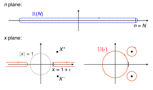
Figure 1: Integration contours in the complex $n$ and $x$ planes, showing finite cutoffs $\left|n\right|\leq N$ and $\left|x\right|>1+\epsilon$. (We do not attempt show the distinction between heavy and light modes for the old and new old sums.) The first contour in the $x$ plane is unwrapped to give the second, containing $\mathbb{U}(\epsilon)$, after reversing its orientation.

In order to distinguish the old and new sums, we must be careful about their upper limits. Let us write $\mathbb{R}(N)$ for the contour encircling the integers up to $\pm N$, and $\mathbb{U}(\epsilon)$ for a unit circle at radius $1+\epsilon$.

• The new sum (28) turns out to be the simplest case. Following the above steps, we write:

  $$\delta E_{\mathrm{new}} =\lim_{N\to\infty}\frac{1}{2}\left(\sum_{n=-N}^{N}\omega_{n}^{\mathrm{heavy}}+\sum_{n=-N/2}^{N/2}\omega_{n}^{\mathrm{light}}\right)$$

  $$=\lim_{N\to\infty}\frac{1}{4i}\left(\oint_{\mathbb{R}(N)}dn\,\cot(\pi n)\,\omega_{n}^{\mathrm{heavy}}+\oint_{\mathbb{R}(N/2)}dn\,\cot(\pi n)\,\omega_{n}^{\mathrm{light}}\right)$$

  $$=\lim_{\epsilon\to 0}-\frac{1}{4i}\oint_{\mathbb{U}(\epsilon)}dx\sum_{ij}(-1)^{F_{ij}}\frac{q^{\prime}_{i}(x)-q^{\prime}_{j}(x)}{2\pi}\cot\left(\frac{q_{i}(x)-q_{j}(x)}{2}\right)\Omega_{ij}(x)$$

  $$\approx-\frac{1}{8\pi i}\sum_{\pm}\pm i\int_{\mathbb{U}_{\pm}}dx\sum_{ij}(-1)^{F_{ij}}\left[\vphantom{\frac{a}{a}}q^{\prime}_{i}(x)-q^{\prime}_{j}(x)\right]\Omega_{ij}(x).$$ (38)

  Since we have the same contour $\mathbb{U}(\epsilon)$ for both heavy and light modes, we can write them as one integral. The last line is the leading term in the expansion (37).

• For the alternative new sum (29),

  $$\delta E_{\mathrm{new}^{\prime}} =\lim_{N\to\infty}\frac{1}{2}\Bigg{(}\sum_{\begin{subarray}{c}n=-2N\\ n\>\mathrm{even}\end{subarray}}^{2N}2\omega_{n}^{\mathrm{heavy}}+\sum_{n=-N}^{N}\omega_{n}^{\mathrm{light}}\Bigg{)}$$

  $$=\lim_{N\to\infty}\frac{1}{4i}\left(\oint_{\mathbb{R}(2N)}dn\,\cot\negmedspace\left(\frac{\pi n}{2}\right)\omega_{n}^{\mathrm{heavy}}+\oint_{\mathbb{R}(N)}dn\,\cot(\pi n)\,\omega_{n}^{\mathrm{light}}\right)$$

  $$=\lim_{\epsilon\to 0}-\frac{1}{4i}\oint_{\mathbb{U}(\epsilon)}dx\sum_{ij}(-1)^{F_{ij}}\frac{q^{\prime}_{i}(x)-q^{\prime}_{j}(x)}{2\pi}\begin{cases}\cot(\frac{q_{i}(x)-q_{j}(x)}{4})\Omega_{ij}(x),&(i,j)\mbox{ heavy}\\ \cot(\frac{q_{i}(x)-q_{j}(x)}{2})\Omega_{ij}(x),&(i,j)\mbox{ light}\end{cases}$$

  $$\approx-\frac{1}{8\pi i}\sum_{\pm}\pm i\int_{\mathbb{U}_{\pm}}dx\sum_{ij}(-1)^{F_{ij}}\left[\vphantom{\frac{a}{a}}q^{\prime}_{i}(x)-q^{\prime}_{j}(x)\right]\Omega_{ij}(x).$$ (39)

  Notice that the difference between this and the new sum (i.e. the argument of the cotangent) disappears in the leading term of (37).

• Finally, for the old sum (26),

  $$\negthickspace\negthickspace\delta E_{\mathrm{old}} =\lim_{N\to\infty}\frac{1}{2}\sum_{n=-N}^{N}\left(\omega_{n}^{\mathrm{heavy}}+\omega_{n}^{\mathrm{light}}\right)$$

  $$=\lim_{N\to\infty}\frac{1}{4i}\oint_{\mathbb{R}(N)}dn\cot(\pi n)\left(\omega_{n}^{\mathrm{heavy}}+\omega_{n}^{\mathrm{light}}\right)$$

  $$=\lim_{\epsilon\to 0}\frac{-1}{4i}\Bigg{\{}\oint_{\mathbb{U}(2\epsilon)}\negthickspace\negthickspace\negthickspace dx\negthickspace\sum_{\begin{subarray}{c}ij\\ \mathrm{heavy}\end{subarray}}+\oint_{\mathbb{U}(\epsilon)}\negthickspace\negthickspace\negthickspace dx\negthickspace\sum_{\begin{subarray}{c}ij\\ \mathrm{light}\end{subarray}}\Bigg{\}}(-1)^{F_{ij}}\frac{q^{\prime}_{i}(x)-q^{\prime}_{j}(x)}{2\pi}\cot\left(\frac{q_{i}(x)-q_{j}(x)}{2}\right)\Omega_{ij}(x)$$

  $$\approx\lim_{\epsilon\to 0}\left[\vphantom{\frac{a}{a}}L^{\mathrm{heavy}}(2\epsilon)+L^{\mathrm{light}}(\epsilon)\right]$$ (40)

  where in the last line we write the leading term of (37) in terms of the integral

  $$L^{\mathrm{light}}(\epsilon) =-\frac{1}{8\pi i}\sum_{\pm}\pm i\int_{\mathbb{U}_{\pm}(\epsilon)}dx\sum_{\begin{subarray}{c}ij\\ \mathrm{light}\end{subarray}}(-1)^{F_{ij}}\left[\vphantom{\frac{a}{a}}q^{\prime}_{i}(x)-q^{\prime}_{j}(x)\right]\Omega_{ij}(x).$$ (41)

  We will explicitly perform this integral along contours of two different radii, $1+\epsilon$ and $1+2\epsilon$, and add them before taking the limit $\epsilon\to 0$.

2.6 Subleading terms

In (38), (39) and (40) above, we kept only the first term in the expansion (37). We now consider the next term, which we call $\delta E^{1}$.

• For the new sum, we have (integrating by parts)

  $$\delta E_{\mathrm{new}}^{1} =-\frac{1}{8\pi i}\sum_{\pm}\int_{\mathbb{U}_{\pm}}dx\sum_{ij}(-1)^{F_{ij}}\partial_{x}\left[q_{i}(x)-q_{j}(x)\right]\left(\pm i2e^{\mp i(q_{i}-q_{j})}\right)\Omega_{ij}(x)$$

  $$=-\frac{1}{4\pi i}\sum_{\pm}\int_{\mathbb{U}_{\pm}}dx\sum_{ij}(-1)^{F_{ij}}e^{\mp i(q_{i}-q_{j})}\partial_{x}\Omega_{ij}(x).$$ (42)

• For the alternative new sum, the only change is in the exponent for the heavy modes:

  $$\negthickspace\negthickspace\negthickspace\negthickspace\delta E_{\mathrm{new}^{\prime}}^{1} =-\frac{1}{8\pi i}\oint_{\mathbb{U}}dx\sum_{ij}(-1)^{F_{ij}}\partial_{x}\left[q_{i}(x)-q_{j}(x)\right]\begin{cases}\left(\pm i2e^{\mp i\frac{q_{i}-q_{j}}{2}}\right)\Omega_{ij}(x),&(i,j)\mbox{ heavy}\\ \left(\pm i2e^{\mp i(q_{i}-q_{j})}\right)\Omega_{ij}(x),&(i,j)\mbox{ light}\end{cases}$$

  $$\negthickspace\negthickspace\negthickspace\negthickspace=-\frac{1}{4\pi i}\sum_{\pm}\int_{\mathbb{U}_{\pm}}dx\Bigg{[}\sum_{\begin{subarray}{c}ij\\ \mathrm{heavy}\end{subarray}}(-1)^{F_{ij}}e^{\mp i\frac{q_{i}-q_{j}}{2}}2\partial_{x}\Omega_{ij}(x)+\sum_{\begin{subarray}{c}ij\\ \mathrm{light}\end{subarray}}(-1)^{F_{ij}}e^{\mp i(q_{i}-q_{j})}\partial_{x}\Omega_{ij}(x)\Bigg{]}.$$ (43)

• And finally, for the old sum, the only difference from the new sum is in the contour $\mathbb{U}(2\epsilon)$ for the heavy modes:

  $$\delta E_{\mathrm{old}}^{1} =-\frac{1}{4\pi i}\sum_{\pm}\Bigg{\{}\int_{\mathbb{U}_{\pm}(2\epsilon)}\negthickspace\negthickspace dx\sum_{\begin{subarray}{c}ij\\ \mathrm{heavy}\end{subarray}}+\int_{\mathbb{U}_{\pm}(\epsilon)}\negthickspace\negthickspace dx\sum_{\begin{subarray}{c}ij\\ \mathrm{light}\end{subarray}}\Bigg{\}}(-1)^{F_{ij}}e^{\mp i(q_{i}-q_{j})}\partial_{x}\Omega_{ij}(x).$$ (44)

We can continue with the higher terms in (37), and calling their total $\delta E^{F}$, write

$$\delta E_{\mathrm{new}}^{F}=\sum_{m=1,2,3\ldots}\frac{-1}{4\pi i}\sum_{\pm}\int_{\mathbb{U}_{\pm}}dx\sum_{ij}(-1)^{F_{ij}}e^{\mp mi(q_{i}-q_{j})}\frac{1}{m}\partial_{x}\Omega_{ij}(x).$$ (45)

Similar expressions can clearly be written down for the old and the alternative new sums.

3 Corrections for the Elementary Giant Magnon

Here we study the solution constructed in the $\sigma$-model by [4, 25] and in the algebraic curve by [3, 33]. This is also known as the small or $CP^{2}$ giant magnon.

3.1 Classical curve

The magnon is described by the algebraic curve

$$q_{1}(x) =\dfrac{\alpha x}{x^{2}-1}$$

$$q_{2}(x) =\dfrac{\alpha x}{x^{2}-1}$$

$$q_{3}(x) =\dfrac{\alpha x}{x^{2}-1}+G(0)-G(\tfrac{1}{x})-\frac{p}{2}$$ (46)

$$q_{4}(x) =\dfrac{\alpha x}{x^{2}-1}+G(x)-\frac{p}{2}$$

$$q_{5}(x) =G(x)-G(0)+G(\tfrac{1}{x})$$

where $p=-i\log(X^{+}/X^{-})$ and the resolvent is [43, 44, 45]

$$G(x)=G_{\mathrm{mag}}(x)=-i\log\left(\frac{x-X^{+}}{x-X^{-}}\right).$$ (47)

Here we have included the twists in $q_{3}(x)$ and $q_{4}(x)$ as used by [42, 46] which amount to orbifolding the space by an angle $p$ so as to make the giant magnon a closed string [47, 48, 49]. Note that these twists play no role in the leading corrections, but are important in the subleading corrections.

The charges $E$ and $Q$ can be read off from the behaviour of $q(x)$ at infinity, see (68) below, and are given in terms of $X^{\pm}$ by

$$E=\Delta-\frac{J}{2} =-ig\left(X^{+}-\frac{1}{X^{+}}-X^{-}+\frac{1}{X^{-}}\right)$$

$$Q =-i2g\left(X^{+}+\frac{1}{X^{+}}-X^{-}-\frac{1}{X^{-}}\right).$$ (48)

These can be combined to give the dispersion relation (1).

3.2 Off-shell frequencies

For the $(1,5)$ polarisation we use the following ansatz, with $\alpha(y)$ and $M(x)$ defined in (12) and (13) above:

$$\delta q_{1} =\frac{\alpha(y)}{x-y}+\sum_{\pm}\frac{a_{\pm}}{x\pm 1} \negthickspace\negthickspace\negthickspace\negthickspace\negthickspace\negthickspace\negthickspace\negthickspace\negthickspace\negthickspace\delta q_{2} =-\delta q_{1}(\tfrac{1}{x})$$

$$\delta q_{4} =\sum_{\pm}\frac{a_{\pm}}{x\pm 1}+M(x) \negthickspace\negthickspace\negthickspace\negthickspace\negthickspace\negthickspace\negthickspace\negthickspace\negthickspace\negthickspace\delta q_{3} =-\delta q_{4}(\tfrac{1}{x})$$ (49)

$$\delta q_{5} =\frac{\alpha(y)}{x-y}+\frac{\alpha(y)}{\frac{1}{x}-y}+\frac{\alpha(y)}{y}+M(x)-M(0)+M(\tfrac{1}{x}).\negthickspace\negthickspace\negthickspace\negthickspace\negthickspace\negthickspace\negthickspace\negthickspace\negthickspace\negthickspace$$

This clearly has the correct new poles and satisfies the inversion symmetries, and also has synchronised poles at $x=\pm 1$. It remains to impose the conditions at infinity, starting with the conditions that $\delta q_{i}$ vanish there. The nontrivial ones are:

$$\delta q_{2}(\infty) =\frac{\alpha(y)}{y}-a_{+}+a_{-}=0$$

$$\delta q_{3}(\infty) =-M(0)-a_{+}+a_{-}=0$$

which, recalling that $M(x)=\sum_{\pm}A^{\pm}/(x-X^{\pm})$, imply

$$\frac{A^{+}}{X^{+}}+\frac{A^{-}}{X^{-}}=\frac{\alpha(y)}{y}.$$ (50)

Next, the $1/x$ behaviour gives the following equations (not all independent):

$$\delta q_{1}(x) \sim\frac{1}{x}\left[\vphantom{\frac{a}{b}}a_{+}+a_{-}+\alpha(y)\right]\;=\frac{\delta\Delta+1}{2gx}$$

$$\delta q_{2}(x) \sim\frac{1}{x}\left[a_{+}+a_{-}+\frac{\alpha(y)}{y^{2}}\right]\;=\frac{\delta\Delta}{2gx}$$

$$\delta q_{3}(x) \sim\frac{1}{x}\left[\vphantom{\frac{a}{b}}a_{+}+a_{-}+A^{+}+A^{-}\right]\;=0$$

$$\delta q_{4}(x) \sim\frac{1}{x}\left[a_{+}+a_{-}+\frac{A^{+}}{X^{+2}}+\frac{A^{-}}{X^{-2}}\right]\;=0$$

$$\delta q_{5}(x) \sim\frac{1}{x}\left[-\alpha(y)+\frac{\alpha(y)}{y^{2}}+A^{+}+A^{-}-\frac{A^{+}}{X^{+2}}-\frac{A^{-}}{X^{-2}}\right]\;=-\frac{1}{2gx}.$$

Using the $\delta q_{2}$ and $\delta q_{4}$ equations we can write $\delta\Delta$ in terms of $y$, $X^{\pm}$ and $A^{\pm}$:

$$\frac{\delta\Delta}{2g}=\frac{\alpha(y)}{y^{2}}-\left(\frac{A^{+}}{X^{+2}}+\frac{A^{-}}{X^{-2}}\right).$$ (51)

The $\delta q_{5}$ equation gives

$$A_{+}+A_{-}=\frac{A^{+}}{X^{+2}}+\frac{A^{-}}{X^{-2}}$$ (52)

which we can use with (50) to find $A^{\pm}$: first write

$$A^{+}=\frac{\alpha(y)}{y}X^{+}-\frac{A^{-}X^{+}}{X^{-}}.$$

and then plugging this into (52) we find

$$A^{-} =-\frac{\alpha(y)}{y}\frac{\left(X^{+2}-1\right)X^{-2}}{\left(X^{-}-X^{+}\right)\left(X^{-}X^{+}+1\right)},$$

$$A^{+} =\frac{\alpha(y)}{y}X^{+}+\frac{\alpha(y)}{y}\frac{\left(X^{+2}-1\right)X^{-}X^{+}}{\left(X^{-}-X^{+}\right)\left(X^{-}X^{+}+1\right)}.$$ (53)

We can now finally write the frequency $\Omega_{15}(y)$ from (51):

$$\Omega_{15}(y)=\delta\Delta =\frac{2g\alpha(y)}{y^{2}}\left[1+y\left(\frac{\left(X^{+2}-1\right)}{\left(X^{-}-X^{+}\right)\left(X^{-}X^{+}+1\right)}\left(1-\frac{X^{-}}{X^{+}}\right)-\frac{1}{X^{+}}\right)\right]$$

$$=\frac{1}{y^{2}-1}\left(1-y\frac{X^{+}+X^{-}}{X^{+}X^{-}+1}\right).$$

For the $(4,5)$ polarisation, we use a similar ansatz

$$\delta q_{1} =\sum_{\pm}\frac{a_{\pm}}{x\pm 1} \negthickspace\negthickspace\negthickspace\negthickspace\negthickspace\negthickspace\negthickspace\negthickspace\negthickspace\negthickspace\delta q_{2} =-\delta q_{1}(\tfrac{1}{x})$$

$$\delta q_{4} =-\frac{\alpha(x)}{x-y}+\sum_{\pm}\frac{a_{\pm}}{x\pm 1}+M(x) \negthickspace\negthickspace\negthickspace\negthickspace\negthickspace\negthickspace\negthickspace\negthickspace\negthickspace\negthickspace\delta q_{3} =-\delta q_{4}(\tfrac{1}{x})$$

$$\delta q_{5} =\frac{\alpha(y)}{x-y}+\frac{\alpha(y)}{\frac{1}{x}-y}+\frac{\alpha(y)}{y}+M(x)-M(0)+M(\tfrac{1}{x})\negthickspace\negthickspace\negthickspace\negthickspace\negthickspace\negthickspace\negthickspace\negthickspace\negthickspace\negthickspace$$

and a similar computation leads to the same frequency:

$$\Omega_{45}(y)=\frac{1}{y^{2}-1}\left(1-y\frac{X^{+}+X^{-}}{X^{+}X^{-}+1}\right).$$

Constructing all the other frequencies using the formulae of section 2.2, we find simply:

$$\Omega_{ij}(y)=\begin{cases}\Omega_{45}(y),&(i,j)\mbox{ light}\\ 2\Omega_{45}(y),&(i,j)\mbox{ heavy}.\end{cases}$$ (54)

This differs from the $AdS_{5}\times S^{5}$ case only by the factor of 2 in the heavy modes, and agrees with the big giant magnon calculation of [33].

3.3 Leading energy corrections

Here we calculate the integrals described in section 2.5. We begin by noting the following identity, which follows simply from the list of possible polarisations (8):

$$\sum_{\begin{subarray}{c}ij\\ \mathrm{heavy}\end{subarray}}(-1)^{F_{ij}}\left[\vphantom{\frac{a}{a}}q^{\prime}_{i}-q^{\prime}_{j}\right] \;=\;q^{\prime}_{1}+q^{\prime}_{2}-q^{\prime}_{3}-q^{\prime}_{4}\;=\;-\frac{1}{2}\sum_{\begin{subarray}{c}ij\\ \mathrm{light}\end{subarray}}(-1)^{F_{ij}}\left[\vphantom{\frac{a}{a}}q^{\prime}_{i}-q^{\prime}_{j}\right].$$ (55)

Using this result, the new sums are trivial, because thanks to the factor 2 in (54), the integrands in both (38) and (39) vanish:

$$\sum_{ij}(-1)^{F_{ij}}\left[\vphantom{\frac{a}{a}}q^{\prime}_{i}(x)-q^{\prime}_{j}(x)\right]\Omega_{ij}(x)=0.$$

So we have, at leading order,

$$\delta E_{\mathrm{new}}=\delta E_{\mathrm{new}^{\prime}}=0.$$ (56)

We wrote the old sum in (40) in terms of two integrals $L^{\mathrm{w}}(\epsilon)$. Using identity (55) and $\Omega_{ij}(y)$ from (54), we see that

$$L^{\mathrm{heavy}}(\epsilon)=-L^{\mathrm{light}}(\epsilon).$$

Using the explicit classical curve (46), we also have

$$q^{\prime}_{1}(x)+q^{\prime}_{2}(x)-q^{\prime}_{3}(x)-q^{\prime}_{4}(x)=i\left(\frac{1}{x-X^{+}}-\frac{1}{x-X^{-}}\right)-i\left(\frac{1}{xX^{+}-1}-\frac{1}{xX^{-}-1}\right).$$

We can now evaluate the integral explicitly, keeping $\epsilon$ finite: parametrise $x=(1+\epsilon)e^{i\varphi}$, where $\varphi\in[0,\pi]$ in $\mathbb{U}_{+}(\epsilon)$ and $\varphi\in[\pi,2\pi]$ in $\mathbb{U}_{-}(\epsilon)$. Then

$$L^{\mathrm{light}}(\epsilon) =\frac{-1}{8\pi i}\sum_{\pm}\pm i\int_{\mathbb{U}_{\pm}(\epsilon)}dx\sum_{\begin{subarray}{c}ij\\ \mathrm{light}\end{subarray}}(-1)^{F_{ij}}\left[\vphantom{\frac{a}{a}}q^{\prime}_{i}(x)-q^{\prime}_{j}(x)\right]\Omega_{ij}(x)$$

$$=\frac{1}{\pi i(1+X^{+}X^{-})}\left[\vphantom{\frac{A}{B}}2(X^{-}-X^{+})\arctan(1+\epsilon)+2X^{+}X^{-}\arctan(X^{-}\left(1+\epsilon\right))\right.$$

$$\qquad+(X^{-}-X^{+})\log\left(\frac{-(2+\epsilon)}{\epsilon}\right)+X^{+}X^{-}\log\left(\frac{1-X^{+}(1+\epsilon)}{1+X^{+}(1+\epsilon)}\right)$$

$$\qquad\left.+\log\left(\frac{\left(1+\epsilon-X^{-}\right)}{\left(1+\epsilon+X^{-}\right)}\frac{\left(1+\epsilon+X^{+}\right)}{\left(1+\epsilon-X^{+}\right)}\right)\right].$$

Only one term diverges as $\epsilon\to 0$. It is this divergent term which makes the limit in (40) nontrivial, and which leads to the following result for the leading term in $\delta E$:

$$\delta E_{\mathrm{old}} =\lim_{\epsilon\to 0}\left[\vphantom{\frac{a}{a}}L^{\mathrm{heavy}}(2\epsilon)+L^{\mathrm{light}}(\epsilon)\right]$$

$$=\lim_{\epsilon\to 0}\left[\vphantom{\frac{a}{a}}-L^{\mathrm{light}}(2\epsilon)+L^{\mathrm{light}}(\epsilon)\right]$$

$$=\frac{i\log 2}{\pi}\frac{X^{+}-X^{-}}{1+X^{+}X^{-}}.$$ (57)

In the non-dyonic case ($Q=1\ll\sqrt{\lambda}$ thus $X^{\pm}=e^{\pm ip/2}$) this becomes

$$\delta E_{\mathrm{old}}=-\frac{\log 2}{\pi}\sin\frac{p}{2}.$$ (58)

Comparing to the expansion (6) of the dispersion relation, we recover (5):

$$c=-\frac{\log 2}{2\pi}.$$

In summary, the situation for these leading corrections for the giant magnon is exactly the same as for the leading corrections for spinning strings in $AdS$. Either we use the old sum prescription and $c\neq 0$, or we use either of the new sums and $c=0$.

We repeat this analysis for the ‘big’ and $RP^{3}$ giant magnons in appendices B and C, reaching the same conclusion in each case.

Dyonic case

We could write the above result (58) as

$$\delta E_{\mathrm{old}}-\delta E_{\mathrm{new}}=c\,\frac{1}{2}\frac{\partial}{\partial g}E$$ (59)

if we use the classical energy $E$ in terms of $g$ (i.e. in terms of $\lambda$), recalling that $h(\lambda)=2g=\sqrt{\lambda/2}$ at leading order. This is of course exactly the second term in the expansion (6).

Now we observe that this is also true for the dyonic case, provided we hold fixed $p$ and $Q$:

$$E =\sqrt{\frac{Q^{2}}{4}+16g^{2}\sin^{2}\frac{p}{2}}$$

$$\implies\quad\frac{\partial}{\partial g}E =\frac{16g\sin^{2}\frac{p}{2}}{E}=-4i\frac{X^{+}-X^{-}}{1+X^{+}X^{-}}$$ (60)

correctly reproducing (57). We have used (48) to write this in $X^{\pm}$, but we stress that the derivative is not holding $X^{\pm}$ fixed.

We note that the dyonic giant magnon is the first example for which the classical energy which one expands is not proportional to $h(\lambda)$. This fact made the expansions for both the $AdS_{3}$ string (4) and (in the strong coupling limit) the non-dyonic giant magnon (6) much simpler than this one.

3.4 Subleading corrections

Consider first the new sum prescription, for which we need to evaluate (42). Using (46), and taking the non-dyonic case $X^{\pm}=e^{\pm ip/2}$, we can write the following pieces of that integral:

$$F_{\mathrm{heavy}}^{+}=\sum_{\begin{subarray}{c}ij\\ \mathrm{heavy}\end{subarray}}(-1)^{F_{ij}}e^{-i\left[q_{i}(x)-q_{j}(x)\right]} =e^{-2i\frac{\alpha x}{x^{2}-1}}\frac{(x+1)\left(e^{ip/2}-1\right)\left(e^{ip/2}(3+x)-(3x+1)\right)}{\left(x-e^{ip/2}\right)^{2}}$$

$$F_{\mathrm{light}}^{+}=\sum_{\begin{subarray}{c}ij\\ \mathrm{light}\end{subarray}}(-1)^{F_{ij}}e^{-i\left[q_{i}(x)-q_{j}(x)\right]} =e^{-i\frac{\alpha x}{x^{2}-1}}\frac{4(x+1)\left(e^{ip/2}-1\right)}{x-e^{ip/2}}.$$ (61)

The contribution from the heavy modes will clearly be subleading to that from the light modes, so we need only consider the latter. The resulting expression for $\delta E^{F,1}$ agrees with that in [33]. This can be integrated using the saddle point at $x=i$ to give [40]:

$$\delta E_{\mathrm{new}}^{F,1}=e^{-\Delta/\sqrt{2\lambda}}\sqrt{\frac{2\,\sqrt{2\lambda}}{\pi\>\Delta}}\left(\frac{\cos\frac{p}{2}}{1-\sin\frac{p}{2}}-1\right).$$ (62)

This term was also calculated by [40] using the Lüscher method, obtaining exactly the same answer. That calculation is really in terms of $h(\lambda)$ not $\lambda$; however this comparison tests only the leading order part of (2), $h(\lambda)=\sqrt{\lambda/2}$, and tells us nothing about $c$.

Now consider the other sums:

• For the old sum, the change in (44) is that while we integrate the light modes at $\epsilon$, for the heavy modes we use $2\epsilon$. At this order we need only note that this will not change the fact that the heavy modes are subleading, and so the answer is the same.

• For the alternative new sum, the change is that for the heavy modes (43) has instead

  $$\sum_{\begin{subarray}{c}ij\\ \mathrm{heavy}\end{subarray}}(-1)^{F_{ij}}e^{-i\frac{q_{i}(x)-q_{j}(x)}{2}}=e^{-i\frac{\alpha x}{x^{2}-1}}\frac{3(x-e^{ip/2})+(x\,e^{ip/2}-1)-4\sqrt{x-e^{ip/2}}\sqrt{x\,e^{ip/2}-1}}{x-e^{ip/2}}.$$

  This is now of the same order as the light modes, and so must be included. Doing so changes the result to

  $$\delta E_{\mathrm{new}^{\prime}}^{F,1}=e^{-\Delta/\sqrt{2\lambda}}\sqrt{\frac{2\,\sqrt{2\lambda}}{\pi\>\Delta}}\left(\frac{2+4\cot\frac{p}{4}}{\cot\frac{p}{4}-1}-4\sqrt{\frac{\cot\frac{p}{4}+1}{\cot\frac{p}{4}-1}}\right)$$ (63)

  which clearly disagrees with the Lüscher result.

To summarise, we obtain the desired subleading correction using either the old or the new sum prescription. However the alternative new sum of [5] gives a mismatching result.

Dyonic case

It is trivial to generalise the above results to the dyonic case. The integrand in (61) becomes

$$F_{\mathrm{light}}^{\pm}(x) =\sum_{\begin{subarray}{c}ij\\ \mathrm{light}\end{subarray}}(-1)^{F_{ij}}e^{\mp i(q_{i}-q_{j})}\partial_{x}\Omega_{45}(x)$$

$$=e^{\mp i\alpha\frac{x}{x^{2}-1}}\left\{e^{\pm ip/2}\left[\left(\frac{x-X^{\mp}}{x-X^{\pm}}\right)^{2}+\left(\frac{x-1/X^{\pm}}{x-1/X^{\mp}}\right)^{2}\right]\left(\frac{x-X^{\pm}}{x-X^{\mp}}+\frac{x-1/X^{\mp}}{x-1/X^{\pm}}\right)\right.$$

$$\qquad\qquad\qquad\left.-2\left(\frac{x-X^{+}}{x-X^{-}}\right)\left(\frac{x-1/X^{+}}{x-1/X^{-}}\right)-2\left(\frac{x-X^{-}}{x-X^{+}}\right)\left(\frac{x-1/X^{-}}{x-1/X^{+}}\right)\right\}\partial_{x}\Omega_{45}(x).$$

The result of integrating this (using the saddle point at $x=i$) is hardly more compact, so we write simply

$$\delta E^{F,1}=\frac{1}{\sqrt{4\pi\alpha}}F_{\mathrm{light}}^{+}(i)$$ (64)

for both the old and the new sums.

3.5 Sub-subleading terms

We can see from (61) that the heavy modes first contribute at order $(e^{-\Delta/\sqrt{2\lambda}})^{2}$. The full correction at this order will also include the contribution of the light modes from the $m=2$ term in (45). The integrand of this term contains (in the non-dyonic limit)

$$F_{\mathrm{light}}^{+2}=\sum_{\begin{subarray}{c}ij\\ \mathrm{light}\end{subarray}}(-1)^{F_{ij}}e^{-2i\left[q_{i}(x)-q_{j}(x)\right]}=e^{-2i\frac{\alpha x}{x^{2}-1}}\frac{4(x^{2}-1)\left(e^{ip}-1\right)}{(x-e^{ip/2})^{2}}.$$

Putting these two contributions together, the correction for the new sum is given by:

$$\delta E_{\mathrm{new}}^{F,2} =-\frac{1}{8\pi i}\sum_{\pm}\int_{\mathbb{U}_{\pm}}dx\sum_{ij}(-1)^{F_{ij}}\left[q^{\prime}_{i}(x)-q^{\prime}_{j}(x)\right]\begin{cases}\left(\pm i2e^{\mp 2i(q_{i}-q_{j})}\right)\Omega_{ij}(x),&(i,j)\mbox{ heavy}\\ \left(\pm i2e^{\mp i(q_{i}-q_{j})}\right)\Omega_{ij}(x),&(i,j)\mbox{ light}\end{cases}$$

$$=-\frac{1}{2\pi i}\int_{\mathbb{U}_{+}}dx\Biggl{[}\sum_{\begin{subarray}{c}ij\\ \mathrm{light}\end{subarray}}(-1)^{F_{ij}}\frac{1}{2}e^{-2i(q_{i}-q_{j})}\partial_{x}\Omega_{ij}(x)+\sum_{\begin{subarray}{c}ij\\ \mathrm{heavy}\end{subarray}}(-1)^{F_{ij}}e^{-i(q_{i}-q_{j})}\partial_{x}\Omega_{ij}(x)\Biggr{]}$$

$$=-\frac{1}{2\pi i}\int_{\mathbb{U}_{+}}dx\left[\frac{1}{2}\;F_{\mathrm{light}}^{+2}\;\Omega_{45}^{\prime}(x)+F_{\mathrm{heavy}}^{+}\;2\Omega_{45}^{\prime}(x)\right]$$

$$=e^{-2\Delta/\sqrt{2\lambda}}\;2\sqrt{\frac{\sqrt{2\lambda}}{\Delta\>\pi}}\left(\frac{\cos\frac{p}{2}-1}{\sin\frac{p}{2}-1}\right).$$ (65)

For the old sum, the essential point to notice is that the heavy and light terms above each lead to a finite contribution, and thus we may take the limits $\epsilon\to 0$ individually. This removes the only distinction between the new and the old sum here, and so we obtain the same result:

$$\delta E_{\mathrm{old}}^{F,2}=\delta E_{\mathrm{new}}^{F,2}.$$

We would not expect $\delta E^{F,2}$ to depend on the value of $c$, since like the subleading term $\delta E^{F,1}$ it is the first term in a series in $1/\sqrt{\lambda}$. The extra power of $e^{-\Delta/\sqrt{2\lambda}}$ to be sub-subleading makes this a different series, not the second term in the series.

Finally, for the alternative new sum, we will again get a different result, just as for the $\delta E^{F,1}$ term in (63) above.

4 Conclusions

All calculations of the $AdS_{4}\times CP^{3}$ interpolating function $h(\lambda)$ work by comparing an expansion in $h(\lambda)$, coming from some integrable structure, to an expansion in $\lambda$, coming from either gauge theory (expanding about $\lambda=0$) or string theory (about $\lambda=\infty$). Such comparisons include:

• The gauge theory calculations of [10, 11] use the exact dispersion relation and draw Feynman diagrams up to four loops, order $\lambda^{4}$.

• For $AdS_{3}$ spinning strings an expansion of the Bethe equations [12] is compared to a semiclassical calculation using either the worldsheet sigma-model [14, 15, 16] or algebraic curves [20].

• The leading ($J=\infty$) corrections for giant magnons in this paper (and in [33]) are computed using the algebraic curve, and compared with the exact dispersion relation (1).

• For finite-$J$ corrections we can compare instead to the Lüscher formulae, which take as input the all-loop S-matrix of [50]. This S-matrix is constructed to agree with the all-loop Bethe ansatz, and thus similarly contains $h(\lambda)$.

In all of these cases, analogous calculations have been done in $AdS_{5}\times S^{5}$, and always agree with the trivial interpolating function $h(\lambda)=\lambda$. Indeed, such comparisons essentially constitute the experimental evidence for the simple form of the interpolating function for this theory [26, 6]. There is also an argument [51] that S-duality fixes the form of $h(\lambda)$ exactly; this is not expected to exist in the $AdS_{4}\times CP^{3}$ case.

Higher-order perturbative checks have also been done, and a strong-coupling result which would be particularly valuable to have here is the two-loop comparison of spinning strings in $AdS_{5}$ with the Bethe ansatz [52, 53, 54]. At two loops, the $AdS_{4}$ radius is expected to receive corrections [23], so one would potentially learn about these in addition to the next term in $h(\lambda)$.

Like the Bethe ansatz which they generalise, the recently proposed TBA and Y-system descriptions [58, 59, 60] are in terms of $h(\lambda)$ rather than $\lambda$. It is in order to be able to translate new results from such descriptions back into the original string- or field-theory language that we need to know about $h(\lambda)$.

4.1 Results at $J=\infty$

We calculated the one-loop energy correction for infinite-$J$ giant magnons using three different summation prescriptions, which we called old, new [20], and alternative new [5]. We find that one can either

• use the old sum prescription and set $c=-\log(2)/2\pi$, or

• use either of the new sum prescriptions and set $c=0$.

This is precisely the same scheme-dependence as was seen for spinning strings in $AdS$. We obtain it however from strings moving only in $CP^{3}$, whose one-loop corrections are finite, rather than growing as $\log S$, and are functions of two variables ($p$ and $Q$, encoded in $X^{\pm}$).

On a technical level, this scheme-dependence comes from a logarithmic divergence in the sum over heavy or light modes alone, which cancels between them. The contributions of heavy and light modes are the two terms in (57):

$$\delta E =\lim_{\epsilon\to 0}\left[\vphantom{\frac{a}{b}}-L(\epsilon_{\mathrm{heavy}})+L(\epsilon)\right]$$

$$\quad\mbox{where }L(\epsilon)=\frac{1}{i\pi}\Big{(}\frac{X^{+}-X^{-}}{1+X^{+}X^{-}}\Big{)}\log\epsilon+\mbox{finite terms},$$

and $\epsilon_{\mathrm{heavy}}=\epsilon$ for either new sum, $\epsilon_{\mathrm{heavy}}=2\epsilon$ for the old sum.

A similar cancellation of logarithmic divergences between heavy and light modes lies behind the finite results of the $AdS_{3}$ spinning string calculations of [14, 15, 16, 22] (using the old sum) and [20] (new sum), even though these papers display only the combined, finite, results.

The heavy modes are something of a puzzle, since the Bethe equations refer only the light modes (4 bosons and 4 fermions) while the string theory treats all 10 dimensions alike. In the formalism used here, each heavy mode is constructed off-shell as the sum of two light modes, (24). However we note that this is not true for the on-shell modes whose frequencies enter into the energy correction.

It has been argued that when loop corrections are taken into account, the heavy states dissolve into the continuum of two-particle states [61], see also [62, 63, 64]. However the fact that they are not stable particles in the interacting theory does not imply that they should be omitted from the path integral, and indeed the present calculation requires that they be included in order to obtain a finite result.

Finally, we observe that it is the old sum which comes closest to imposing a physical cutoff, treating all modes on an equal footing. The frequencies $\omega=\Omega(x)$ computed here are frequencies with respect to physical time. Unlike the mode number (or worse, the position in the spectral plane) this is a local quantity on the worldsheet. If we explicitly choose the same cutoff for heavy and light modes, by setting $\Omega_{\mathrm{heavy}}(1+\epsilon_{\mathrm{heavy}})=\Omega_{\mathrm{light}}(1+\epsilon)=\Lambda$, then the vacuum’s frequencies (33) lead us to

$$\epsilon_{\mathrm{heavy}}=2\epsilon+\mathcal{O}(\epsilon^{2}).$$

Using instead the giant magnon’s frequencies (54) gives no change at this order. And from the point of view of the calculation of $\delta E$ in (57), this physical condition is equivalent to the old sum, (40).

4.2 Finite-$J$ effects

Following [42, 39] we can summarise the complete energy of a giant magnon, including the various finite $J$ (thus finite $\Delta$) corrections, as follows:

$$E=\negthickspace\negthickspace\sum_{m,n=0,1,2\ldots}\negthickspace\negthickspace a_{m,n}\left(e^{-\Delta/\sqrt{2\lambda}}\right)^{m}\left(e^{-2\Delta/E}\right)^{n}.$$ (66)

Each of the coefficients $a_{m,n}$ is a series in $1/\sqrt{\lambda}$, and the leading corrections discussed above are part of $a_{0,0}=E_{\mathrm{class}}+\delta E+o(1/\sqrt{\lambda})$.

The coefficients $a_{m,0}$ are classically zero. Calculating $a_{1,0}$ at one-loop (order $\sqrt{\lambda}^{0}$) following [42] we see no difference between the old and new sums, and find agreement with the Lüscher method calculation of [40]. (There these are referred to as F-terms, and arise from virtual particles travelling full circle around the worldsheet.) However for the alternative new sum of [5], we find a disagreement. In this case both heavy and light modes contribute. For the old and new sums, $a_{1,0}$ depends only on the light modes, with heavy modes first entering in $a_{2,0}$, which we also calculate, (65).

The coefficient $a_{0,1}$ contains the classical (order $\sqrt{\lambda}$) corrections to the magnon’s energy, of they type studied by [66, 47, 67, 68] and, using algebraic curves, by [72, 34, 4]. Its one-loop part was calculated for the $AdS_{5}\times S^{5}$ case by [39], who found agreement with the subleading Lüscher $\mu$-term calculation of [73]. The analogue of their calculation is useful to us here because, like $a_{0,0}$, the one-loop corrections give us the second term in the series in $1/\sqrt{\lambda}$, and so we can potentially learn about $c$.

In order to calculate the relevant quantum corrections, we need to start with the algebraic curve for a classical finite-$J$ giant magnon. This, and the need to keep various terms we ignored before, adds considerable complication [39]. In addition not all of the Lüscher terms one would like to compare to are known. Thus far we can report that:

• The leading bound-state $\mu$-term matches perfectly with the classical algebraic curve result of [4] for one dyonic elementary magnon.

• The subleading $\mu$-terms of [40] for the $RP^{3}$ magnon can be recovered from the one-loop algebraic curve by calculating $a_{0,1}$ using the new sum.

• When calculating $a_{0,1}$ using the old sum (40), it has a linear divergence in the cutoff $N$.

These and other related calculations are the material of a forthcoming paper.

Acknowledgements

From the inception of this project, we thank an anonymous referee of the paper [40], and the organisers of the Potsdam IGST conference, July 2009. Along the way, we thank C. Ahn, D. Fioravanti, M. Kim and S. Minwalla for discussions.

For hospitality while working on this, MCA thanks Wits (Johannesburg) and IST (Lisbon), IA thanks TIFR (Mumbai), and DB thanks IEU (Seoul).

IA was supported in part by the Fundação para a Ciência e a Tecnologia (FCT / Portugal). DB was supported by WCU grant No. R32-2008-000-101300, and by University PRIN 2007JHLPEZ ‘Fisica Statistica dei Sistemi Fortemente Correlati all’Equilibrio e Fuori Equilibrio: Risultati Esatti e Metodi di Teoria dei Campi’.

Appendix A The Classical Algebraic Curve

For completeness we give here some relevant properties. The $AdS_{4}\times CP^{3}$ case was first studied by [3], drawing on past work on $AdS_{5}\times S^{5}$ by [74, 75, 76, 77, 78, 38] among others.

The monodromy matrix is defined from the Lax connection $J(x)$ by

$$\Omega(x)=P\,e^{\oint d\sigma J_{\sigma}(x)}.$$

Here we integrate once around the worldsheet $(\sigma,\tau)$. The connection depends on an arbitrary complex number $x$ called the spectral parameter, and since it is flat (for all $x$) the eigenvalues of $\Omega$ are independent of the path used. We write these as

$$\operatorname{eig}\Omega(x)=\left\{\vphantom{\frac{a}{a}}e^{i\hat{p}_{1}},e^{i\hat{p}_{2}},e^{i\hat{p}_{3}},e^{i\hat{p}_{4}},e^{i\tilde{p}_{1}},e^{i\tilde{p}_{2}},e^{i\tilde{p}_{3}},e^{i\tilde{p}_{4}}\right\}$$

and call to the eight functions $\tilde{p}_{i}$ ($CP$) and $\hat{p}_{i}$ ($AdS$) ‘quasi-momenta’. In order to make the $OSp(2,2|6)$ symmetry explicit, we will work not with $p_{i}$ but instead with ten new quasi-momenta $q_{i}$ defined [3]

$$\Big{(}q_{1},q_{2},q_{3},q_{4},q_{5}\Big{)}=\frac{1}{2}\Big{(}\hat{p}_{1}+\hat{p}_{2},\hat{p}_{1}-\hat{p}_{2},\tilde{p}_{1}+\tilde{p}_{2},-\tilde{p}_{2}-\tilde{p}_{4},\tilde{p}_{1}+\tilde{p}_{4}\Big{)}$$

and $\big{(}q_{6},q_{7},q_{8},q_{9},q_{10}\big{)}=\big{(}-q_{5},-q_{4},-q_{3},-q_{2},-q_{1}\big{)}.$

These functions define a 10-sheeted Riemann surface. It need not however be continuous across branch cuts, so long as $\operatorname{eig}\mathrm{\Omega(x)}$ is continuous: when a cut $C_{ij}$ connects sheets $i$ and $j$, we must have $q_{i}^{+}-q_{j}^{-}=2\pi n$ when $x\in C_{ij}$. There are two additional constraints:

• First, the Virasoro constraints lead to synchronised poles at $x=\pm 1$:

  $$\big{(}q_{1},q_{2},q_{3},q_{4},q_{5}\big{)} =\frac{\alpha_{+}}{(x-1)}\big{(}1,1,1,1,0\big{)}+\mathcal{O}(x-1)^{0}$$

  $$=\frac{\alpha_{-}}{(x+1)}\big{(}1,1,1,1,0\big{)}+\mathcal{O}(x+1)^{0}.$$

• Second, the curve has the following inversion symmetries:

  $$q_{1}(\tfrac{1}{x}) =-q_{2}(x)$$

  $$q_{3}(\tfrac{1}{x}) =2\pi m-q_{4}(x)$$ (67)

  $$q_{5}(\tfrac{1}{x}) =q_{5}(x).$$

  This $m\in\mathbb{Z}$ is the winding number.

The string’s charges are determined by the asymptotic behaviour as $x\to\infty$:

$$\left(\begin{array}[]{c}q_{1}\\ q_{2}\\ q_{3}\\ q_{4}\\ q_{5}\end{array}\right)=\left(\begin{array}[]{c}0\\ 0\\ -p/2\\ -p/2\\ 0\end{array}\right)+\frac{1}{2gx}\left(\begin{array}[]{c}\Delta+S\\ \Delta-S\\ (J+Q)/2\\ (J-Q)/2\\ J_{3}\end{array}\right)+\mathcal{O}\Big{(}\frac{1}{x^{2}}\Big{)}.$$ (68)

The ‘twists’ $p/2$ are the same as we added to the solution (46) to allow for nonzero momentum. In [4] we instead allowed non-integer $m$; this however will get the $F$-terms of section 3.4 wrong.

For each square-root branch cut $C_{ij}$, we define the filling fraction as

$$S_{ij}=\frac{g}{i\pi}\oint_{C_{ij}}dx\left(1-\frac{1}{x^{2}}\right)q_{i}(x).$$ (69)

The new poles which we add when studying fluctuations are very short branch cuts; this is why they connect two sheets $i$ and $j$. The residue $\alpha(y)$ is set by the condition that they are each exactly one fluctuation: $S_{ij}=1$.

Appendix B Corrections for the Big Giant Magnon

The big giant magnon is a two-parameter one-angular-momentum solution, which was known in the algebraic curve [33] before being constructed in the $\sigma$-model [29, 30, 31, 32]. It should be thought of as consisting of two elementary magnons in a particular orientation [25, 32].

The big magnon is described by the algebraic curve

$$q_{1}(x)=q_{2}(x) =\dfrac{\alpha x}{x^{2}-1}$$

$$q_{3}(x)=q_{4}(x) =\dfrac{\alpha x}{x^{2}-1}+G(x)+G(0)-G(\tfrac{1}{x})-p$$

$$q_{5}(x) =0$$

with $G(x)$ as in (47). As for the $RP^{3}$ case, we now adopt conventions in which $2p$ is the total momentum.

B.1 Off-shell frequencies

For the $(1,5)$ polarisation, we use this ansatz:

$$\delta q_{1} =\frac{\alpha(y)}{x-y}+\frac{a_{+}}{x+1}+\frac{a_{-}}{x-1} \delta q_{2} =-\delta q_{1}(\tfrac{1}{x})$$

$$\delta q_{4} =\frac{a_{+}}{x+1}+\frac{a_{-}}{x-1}+M(x)+M(0)-M(\tfrac{1}{x}) \delta q_{3} =-\delta q_{4}(\tfrac{1}{x})$$

$$\delta q_{5} =\frac{\alpha(y)}{x-y}+\frac{\alpha(y)}{\frac{1}{x}-y}+\frac{\alpha(y)}{y}.$$

This clearly has the correct new poles and satisfies the inversion symmetries, and the changes in the residues of the poles at $x=\pm 1$ are all the same. Imposing the conditions at infinity now fixes $a_{\pm}$ and $A^{\pm}$, and we get

$$\Omega_{15}(y)=\delta\Delta=\frac{1}{y^{2}-1}\left(1-y\frac{X^{+}+X^{-}}{1+X^{+}X^{-}}\right).$$

For the $(4,5)$ polarisation,

$$\delta q_{1} =\frac{a}{x+1}+\frac{a}{x-1} \delta q_{2} =-\delta q_{1}(\tfrac{1}{x})$$

$$\delta q_{4} =-\frac{\alpha(y)}{x-y}+\frac{a}{x+1}+\frac{a}{x-1}+M(x)+M(0)-M(\tfrac{1}{x}) \delta q_{3} =-\delta q_{4}(\tfrac{1}{x})$$

$$\delta q_{5} =\frac{\alpha(y)}{x-y}+\frac{\alpha(y)}{\frac{1}{x}-y}+\frac{\alpha(y)}{y}$$

leads to

$$\Omega_{45}(y)=\frac{1}{y^{2}-1}\left(1-y\frac{X^{+}+X^{-}}{1+X^{+}X^{-}}\right).$$

We can then find all the other frequencies, and as before:

$$\Omega_{ij}(y)=\begin{cases}\Omega_{45}(y),&(i,j)\mbox{ light}\\ 2\Omega_{45}(y),&(i,j)\mbox{ heavy}.\end{cases}$$ (70)

This is exactly as in [33], except for notation.

B.2 Energy corrections

Note that identity (55) still holds, and with (70) implies that for the new sum, we get

$$\delta E_{\mathrm{new}}=0.$$

This is the result of [33]. Despite pre-dating [20], this paper uses an integral like (38), and thus has implicitly adopted the new sum (28).

For the old sum, (26), a similar calculation to the one we did for the elementary giant magnon leads to

$$\delta E_{\mathrm{old}}=-2\frac{\log 2}{\pi}\sin\frac{p}{2}$$

twice what we got for the elementary magnon, equation (58), and thus consistent with the same value of $c$.

Appendix C Corrections for the $RP^{3}$ Magnon

The $RP^{3}$ giant magnon, an embedding of Dorey’s $S^{3}$ dyonic giant magnon, is described in the algebraic curve by

$$q_{1}(x)=q_{2}(x) =\dfrac{\alpha x}{x^{2}-1}$$

$$q_{3}(x) =\dfrac{\alpha x}{x^{2}-1}+2G(0)-2G(\tfrac{1}{x})-p$$

$$q_{4}(x) =\dfrac{\alpha x}{x^{2}-1}+2G(x)-p$$

$$q_{5}(x) =0.$$

This is a superposition of two elementary magnons (one ‘u’ and one ‘v’ in [4]). Here $p$ is the momentum of each of the elementary magnons, so that the total momentum is $2p$. The dispersion relation is

$$E =\sqrt{\frac{Q^{2}}{4}+16h(\lambda)^{2}\sin^{2}\frac{p}{2}}$$ (71)

$$=8g\sin\frac{p}{2}\qquad\mbox{when }Q=2\ll\lambda=8g^{2}.$$

In the non-dyonic limit (and at strong coupling) this is simply twice that of the elementary magnon.

The calculation of this one-loop correction is very similar to that for one elementary magnon, so we state results here without showing any detail. Using the new sum, we obtain

$$\delta E_{\mathrm{new}}=0$$

and using the old sum

$$\delta E_{\mathrm{old}}=-2\frac{\log 2}{\pi}\sin\frac{p}{2}$$

exactly twice that for the elementary magnon, and thus consistent with the same value of $c$.

Finally the subleading correction for both old and new sums is

$$\delta E^{F,1} =\frac{1}{\sqrt{\alpha\pi}}e^{-\alpha/2}\left[e^{ip}\frac{X^{+2}(X^{-2}+1)^{2}+X^{-2}(X^{+2}+1)^{2}}{X^{+2}(X^{+}-i)^{2}(X^{-}+i)^{2}}-2\right]$$

$$=\frac{-4}{\sqrt{\alpha\pi}}e^{-\alpha/2}\frac{\sin\frac{p}{2}}{\sin\frac{p}{2}-1}\qquad\mbox{when }Q\ll\sqrt{\lambda}.$$ (72)

In the non-dyonic limit this correction matches the Lüsher F-term calculated by [40]. In this limit the $RP^{3}$ magnon and the big magnon co-incide, and the same integral was also obtained for this term by [33].

Appendix D Conventions and the Vacuum

When defining the frequency $\Omega(y)$ from $\delta\Delta$, the paper [5] writes, instead of our (22),

$$\Omega(y)=\delta\Delta+\sum_{AdS\,\mathrm{modes}}N^{ij}+\frac{1}{2}\sum_{\mathrm{fermions}}N^{ij}.$$ (73)

This change (from our conventions) cancels out of either of the new sums, but not out of the old sum. As a result that paper finds that $\delta E_{\mathrm{old}}=\infty$ for the vacuum. Since the same shifts apply to any soliton solution too, they will cancel out of any normalised energy correction $\delta E-\delta E_{\mathrm{vac}}$. Our conventions have the advantage of producing a much simpler set of frequencies (33). The conventions of [3] agree with those of [5], since they obtain the same frequency shifts although without writing a formula like (73).

We observe that our conventions produce off-shell frequencies which vanish as the new pole is taken to infinity: $\Omega(y\to\infty)=0$.

Similar calculations of the same vacuum frequencies have been done from the worldsheet perspective, either directly [5] or using the Penrose limit [8, 6, 7], obtaining various other constant shifts. We summarise these in table 1.

Note that all of these are only constant shifts added to the frequencies. What the paper [80] discusses is half-integer shifts of $n$, which are much more subtle. The conclusion there was that one has to be very careful to get these right for fermions in the worldsheet calculation.

		Algebraic Curves:			Worldsheet:
	This paper	G&V [3]	B&L [5]	N&T [8]	GGY [6]	GHO [7]	B&L [5]
$AdS$ bosons
heavy $\times 3$	$-1$	0	0	0	0	0	0
Fermions
heavy $\times 4$	$-1$	$-1/2$	$-1/2$	0	0		$\pm 1/2$
light $\times 4$	$-1/2$	0	0	0	0		0
$CP$ bosons
heavy $\times 1$	$-1$	$-1$	$-1$	0	0	0	0
light $\times 4$	$-1/2$	$-1/2$	$-1/2$	0	0	$\pm 1/2$	$\pm 1/2$
Total (weighted)	0	$-1$	$-1$	0	0		0

Table 1: Constant shifts of the vacuum’s fluctuation frequencies. The ‘unshifted’ frequencies are the square root terms in (34) above, and the total of course includes multiplicity and counts fermions with a minus.

Appendix E Momentum Conservation and Level Matching

E.1 The vacuum

When constructing the perturbations $\delta q$ for the vacuum (point particle) solution, the paper [5] used a pair of new poles at $\pm y$, and calculate the total $\delta\Delta=\Omega(y)+\Omega(-y)$. This construction is clearly blind to any terms odd in $y$. However it is justified in this case, since on-shell we have $x_{-n}^{ij}=-x_{n}^{ij}$ for all $ij,n$, and every sum $\delta E$ contains $\omega_{n}+\omega_{-n}$, so such terms cannot affect the result.

Using a pair of excitations $x_{\pm n}^{ij}$ is also sufficient to satisfy the level matching condition (10), although it will not be the only way to do so. The paper [3] states that they always use a pair of poles $x_{\pm n}^{ij}$ for this reason, and for the vacuum case they study this is equivalent to using a pair at $\pm y$.

Another way to construct $\Omega(y)$ is to use just one pole but allow some change in the momentum: for the $(4,5)$ polarisation, we would use this ansatz:

$$\delta q_{1} =\sum_{\pm}\frac{a_{\pm}}{x\pm 1} \delta q_{2} =-\delta q_{1}(\tfrac{1}{x})$$

$$\delta q_{4} =-\frac{\alpha(y)}{x-y}+\sum_{\pm}\frac{a_{\pm}}{x\pm 1} \delta q_{3} =-\delta q_{4}(\tfrac{1}{x})+\delta p$$

$$\delta q_{5} =\frac{\alpha(y)}{x-y}+\frac{\alpha(y)}{\frac{1}{x}-y}+\frac{\alpha(y)}{y}.$$ (74)

This leads to the same frequency as before,

$$\Omega_{45}(y)=\delta\Delta=\frac{1}{y^{2}-1}$$

as well as momentum

$$\delta p=\frac{\alpha(y)}{y}=\frac{1}{2g}\frac{y}{y^{2}-1}.$$ (75)

It is clear that when considering two poles at $\pm y$, the total $\delta p$ will be zero again.

When we construct a heavy fluctuation like this, such as the $(3,7)$ mode, we will get $\delta p=2\alpha(y)/y$. Alternatively recall that we constructed heavy fluctuations in (24) by adding two light fluctuations, and the $\delta p$ will similarly add up.

E.2 Giant magnons

We can repeat our analysis of the giant magnon allowing $\delta p\neq 0$, in the same way as for the vacuum: change the ansatz (49) to have $\delta q_{3}(x)=-\delta q_{4}(\tfrac{1}{x})+\delta p$. We find (writing just the non-dyonic case)

$$\Omega_{45}(y)=\left[\frac{1}{y^{2}-1}-\frac{y}{y^{2}-1}\cos\frac{p}{2}\right]+2g\,\delta p\,\cos\frac{p}{2}.$$ (76)

The first two terms (in square brackets) are the terms appearing in (54). Notice that if we take $\delta p=\alpha(y)/y$ (as for the vacuum) then the new third term here has the same form as the second term — in fact they cancel.

This is a nice demonstration of the argument for the giant magnon’s off-shell frequency $\Omega(y)$ given by [42]. They say that the first term is the energy of the excitation, while the second term comes from the fact that the perturbation carries some momentum $\delta p$, and so if total momentum is conserved, the magnon’s momentum must change to compensate. We can write this as

$$\Omega(y)=E_{\mathrm{excitation}}-\delta p\frac{\partial E_{\mathrm{magnon}}}{\partial p}$$

and we recall that $\partial E/\partial p=2g\cos\frac{p}{2}$ for the non-dyonic case.

We can describe such an excitation using $X^{\pm}$ near to $y$: solving $Q=1$ in (48) we find

$$X^{\pm}=y\pm\frac{i}{4g}\frac{y^{2}}{y^{2}-1}$$

which leads to the same momentum as (75)

$$\delta p=-i\log\frac{X^{+}}{X^{-}}=\frac{1}{2g}\frac{y}{y^{2}-1}.$$

Now consider the effect of the term in $\Omega(y)$ arising from momentum conservation on our calculation of the one-loop correction $\delta E$. If we drop the second term from all $\Omega_{ij}(y)$, there will be no change in the new sum (56). But there is a change in the old sum (57), which becomes

$$\delta E_{\mathrm{old}}=-2\frac{\log 2}{2\pi}\frac{1}{\sin\frac{p}{2}}$$

This is not a term which $c$ could produce in (6).

Had we constructed $\delta q(x)$ starting with a pair of new poles at $\pm y$, we would not have obtained the second term in $\Omega_{ij}(y)$, since it is odd in $y$. For the elementary magnon it is clear that we may not do this, as (9) always involves $G_{\mathrm{mag}}(x)$ which has no simple behaviour under $x\to-x$. But in the case of the big magnon, for the (1,5) polarisation, we may have been tempted: the classical curve’s $q_{1}(x)$ and $a_{5}(x)$ are identical to those of the vacuum. For the $(4,5)$ polarisation, clearly we cannot. Dropping this second term from $\Omega_{15}(y)$ but not from $\Omega_{45}(y)$, and then blindly using section 2.2’s formulae to generate all the rest, we obtain a divergent correction $\delta E$. And our error is that for instance $\Omega_{18}(y)$ has been built using $\Omega_{15}(y)$, and thus a pair of new poles $\pm y$, but for this polarisation the on-shell pole positions are not simply related, $x_{\pm n}^{18}\neq\pm y$.

E.3 Spinning strings

The paper [5] studies quantum corrections for spinning strings with two equal angular momenta. When constructing the fluctuation $\delta q(x)$, it uses a pair of poles at $\pm y$. This is justified for both the $(1,5)$ and the $(4,5)$ polarisations, just as it was for the vacuum.

But it is not justified for all the other polarisations: not all of the on-shell pole positions come in pairs $x_{\pm n}^{ij}=\pm y$. For example the $(1,8)$ polarisation does not have this property. Nevertheless $\Omega_{18}(y)$ is constructed from $\Omega_{15}(y)$ and $\Omega_{45}(y)$.

Attempting to find a way to construct $\delta q(x)$ without using this assumption, we tried allowing both $\delta p$ and for the two endpoints of the square-root cut to move independently. This appears to lead to a valid fluctuation, which adds to the result of [5] the following term in $\Omega_{45}(y)$:

$$i\frac{m}{\mathcal{J}}\frac{K(1/y)}{K(1)}\frac{y}{y^{2}-1}.$$ (77)

The change in the momentum is

$$\delta p=\frac{\alpha(y)}{y}(1-i)\frac{K(1/y)}{\mathcal{J}}.$$ (78)

Here we use that paper’s notation: $K(x)=\sqrt{\mathcal{J}^{2}+m^{2}x^{2}/4}$ is the branch cut term, with $\mathcal{J}$ the angular momentum and $m$ the winding.

It’s not entirely clear what to make of these new terms. We have not tried to work out whether they affect the energy corrections for which agreement was found with worldsheet results.

References

- [1] J. M. Maldacena, The large N limit of superconformal field theories and supergravity, Adv. Theor. Math. Phys. 2 (1998) 231–252 [arXiv:hep-th/9711200].
- [2] O. Aharony, O. Bergman, D. L. Jafferis and J. M. Maldacena, superconformal Chern–Simons-matter theories, M2-branes and their gravity duals, JHEP 10 (2008) 091 [arXiv:0806.1218].
- [3] N. Gromov and P. Vieira, The / algebraic curve, JHEP 02 (2008) 040 [arXiv:0807.0437].
- [4] M. C. Abbott, I. Aniceto and O. Ohlsson Sax, Dyonic giant magnons in : Strings and curves at finite J, Phys. Rev. D80 (2009) 026005 [arXiv:0903.3365].
- [5] M. A. Bandres and A. E. Lipstein, One-loop corrections to type IIA string theory in , JHEP 04 (2010) 059 [arXiv:0911.4061].
- [6] D. Gaiotto, S. Giombi and X. Yin, Spin chains in superconformal Chern–Simons-matter theory, JHEP 04 (2009) 066 [arXiv:0806.4589].
- [7] G. Grignani, T. Harmark and M. Orselli, The sector in the string dual of superconformal Chern–Simons theory, Nucl. Phys. B810 (2008) 115–134 [arXiv:0806.4959].
- [8] T. Nishioka and T. Takayanagi, On type IIA Penrose limit and Chern–Simons theories, JHEP 08 (2008) 001 [arXiv:0806.3391].
- [9] J. A. Minahan and K. Zarembo, The Bethe ansatz for superconformal Chern–Simons, JHEP 09 (2008) 040 [arXiv:0806.3951].
- [10] J. A. Minahan, O. Ohlsson Sax and C. Sieg, Magnon dispersion to four loops in the ABJM and ABJ models, J. Phys. A43 (2010) 275402 [arXiv:0908.2463v3].
- [11] J. A. Minahan, O. Ohlsson Sax and C. Sieg, Anomalous dimensions at four loops in superconformal Chern–Simons theories, arXiv:0912.3460.
- [12] N. Gromov and P. Vieira, The all loop / Bethe ansatz, JHEP 01 (2009) 016 [arXiv:0807.0777].
- [13] S. S. Gubser, I. R. Klebanov and A. M. Polyakov, A semi-classical limit of the gauge/string correspondence, Nucl. Phys. B636 (2002) 99–114 [arXiv:hep-th/0204051].
- [14] T. McLoughlin and R. Roiban, Spinning strings at one-loop in , JHEP 12 (2008) 101 [arXiv:0807.3965].
- [15] L. F. Alday, G. Arutyunov and D. Bykov, Semiclassical quantization of spinning strings in , JHEP 11 (2008) 089 [arXiv:0807.4400].
- [16] C. Krishnan, / at one loop, JHEP 09 (2008) 092 [arXiv:0807.4561].
- [17] S. Frolov and A. A. Tseytlin, Semiclassical quantization of rotating superstring in , JHEP 06 (2002) 007 [arXiv:hep-th/0204226v5].
- [18] I. Y. Park, A. Tirziu and A. A. Tseytlin, Spinning strings in : One-loop correction to energy in sector, JHEP 03 (2005) 013 [arXiv:hep-th/0501203].
- [19] S. Frolov, A. Tirziu and A. A. Tseytlin, Logarithmic corrections to higher twist scaling at strong coupling from AdS/CFT, Nucl. Phys. B766 (2007) 232–245 [arXiv:hep-th/0611269].
- [20] N. Gromov and V. Mikhaylov, Comment on the scaling function in , JHEP 04 (2009) 083 [arXiv:0807.4897].
- [21] G. Arutyunov, S. Frolov and M. Staudacher, Bethe ansatz for quantum strings, JHEP 10 (2004) 016 [arXiv:hep-th/0406256].
- [22] T. McLoughlin, R. Roiban and A. A. Tseytlin, Quantum spinning strings in : testing the Bethe ansatz proposal, JHEP 11 (2008) 069 [arXiv:0809.4038].
- [23] O. Bergman and S. Hirano, Anomalous radius shift in /, JHEP 07 (2009) 016 [arXiv:0902.1743].
- [24] M. C. Abbott and I. Aniceto, Giant magnons in : Embeddings, charges and a Hamiltonian, JHEP 04 (2009) 136 [arXiv:0811.2423].
- [25] T. J. Hollowood and J. L. Miramontes, A new and elementary dyonic magnon, JHEP 08 (2009) 109 [arXiv:0905.2534].
- [26] D. M. Hofman and J. M. Maldacena, Giant magnons, J. Phys. A39 (2006) 13095–13118 [arXiv:hep-th/0604135].
- [27] N. Dorey, Magnon bound states and the AdS/CFT correspondence, J. Phys. A39 (2006) 13119–13128 [arXiv:hep-th/0604175].
- [28] H.-Y. Chen, N. Dorey and K. Okamura, Dyonic giant magnons, JHEP 09 (2006) 024 [arXiv:hep-th/0605155].
- [29] T. J. Hollowood and J. L. Miramontes, Magnons, their solitonic avatars and the Pohlmeyer reduction, JHEP 04 (2009) 060 [arXiv:0902.2405].
- [30] C. Kalousios, M. Spradlin and A. Volovich, Dressed giant magnons on , JHEP 07 (2009) 006 [arXiv:0902.3179].
- [31] R. Suzuki, Giant magnons on by dressing method, JHEP 05 (2009) 079 [arXiv:0902.3368].
- [32] Y. Hatsuda and H. Tanaka, Scattering of giant magnons in , JHEP 02 (2010) 085 [arXiv:0910.5315].
- [33] I. Shenderovich, Giant magnons in /: dispersion, quantization and finite–size corrections, arXiv:0807.2861.
- [34] T. Łukowski and O. Ohlsson Sax, Finite size giant magnons in the sector of , JHEP 12 (2008) 073 [arXiv:0810.1246].
- [35] G. Papathanasiou and M. Spradlin, Semiclassical quantization of the giant magnon, JHEP 06 (2007) 032 [arXiv:0704.2389].
- [36] N. Gromov and P. Vieira, The superstring quantum spectrum from the algebraic curve, Nucl. Phys. B789 (2008) 175–208 [arXiv:hep-th/0703191].
- [37] N. Beisert, J. A. Minahan, M. Staudacher and K. Zarembo, Stringing spins and spinning strings, JHEP 09 (2003) 010 [arXiv:hep-th/0306139].
- [38] N. Beisert, V. A. Kazakov, K. Sakai and K. Zarembo, Complete spectrum of long operators in SYM at one loop, JHEP 07 (2005) 030 [arXiv:hep-th/0503200].
- [39] N. Gromov, S. Schäfer-Nameki and P. Vieira, Efficient precision quantization in AdS/CFT, JHEP 12 (2008) 013 [arXiv:0807.4752].
- [40] D. Bombardelli and D. Fioravanti, Finite-size corrections of the giant magnons: the Lüscher terms, JHEP 07 (2009) 034 [arXiv:0810.0704].
- [41] S. Schäfer-Nameki, Exact expressions for quantum corrections to spinning strings, Phys. Lett. B639 (2006) 571–578 [arXiv:hep-th/0602214].
- [42] N. Gromov, S. Schäfer-Nameki and P. Vieira, Quantum wrapped giant magnon, Phys. Rev. D78 (2008) 026006 [arXiv:0801.3671].
- [43] J. A. Minahan, A. Tirziu and A. A. Tseytlin, Infinite spin limit of semiclassical string states, JHEP 08 (2006) 049 [arXiv:hep-th/0606145].
- [44] B. Vicedo, Giant magnons and singular curves, JHEP 12 (2007) 078 [arXiv:hep-th/0703180].
- [45] H.-Y. Chen, N. Dorey and R. F. L. Matos, Quantum scattering of giant magnons, JHEP 09 (2007) [arXiv:0707.0668].
- [46] N. Gromov and P. Vieira, Complete 1-loop test of AdS/CFT, JHEP 04 (2008) 046 [arXiv:0709.3487].
- [47] D. Astolfi, V. Forini, G. Grignani and G. W. Semenoff, Gauge invariant finite size spectrum of the giant magnon, Phys. Lett. B651 (2007) 329–335 [arXiv:hep-th/0702043].
- [48] K. Ideguchi, Semiclassical strings on and operators in orbifold field theories, JHEP 09 (2004) 008 [arXiv:hep-th/0408014].
- [49] A. Solovyov, Bethe ansatz equations for general orbifolds of SYM, JHEP 04 (2008) 013 [arXiv:0711.1697].
- [50] C. Ahn and R. I. Nepomechie, super Chern–Simons theory S-matrix and all-loop Bethe ansatz equations, JHEP 09 (2008) 010 [arXiv:0807.1924].
- [51] D. Berenstein and D. Trancanelli, S-duality and the giant magnon dispersion relation, arXiv:0904.0444.
- [52] S. Giombi, R. Ricci, R. Roiban, A. A. Tseytlin and C. Vergu, Generalized scaling function from light-cone gauge superstring, JHEP 06 (2010) 60 [arXiv:1002.0018].
- [53] N. Gromov, Generalized scaling function at strong coupling, JHEP 11 (2008) 085 [arXiv:0805.4615].
- [54] R. Roiban and A. A. Tseytlin, Spinning superstrings at two loops: strong-coupling corrections to dimensions of large-twist SYM operators, Phys. Rev. D77 (2008) 066006 [arXiv:0712.2479].
- [55] T. Banks and M. B. Green, Nonperturbative effects in AdS in five-dimensions string theory and d = 4 susy Yang–Mills, JHEP 9805 (1998) 002 [arXiv:hep-th/9804170].
- [56] R. Kallosh, J. Rahmfeld and A. Rajaraman, Near horizon superspace, JHEP 9809 (1998) 002 [arXiv:hep-th/9805217].
- [57] L. Mazzucato and B. C. Vallilo, On the non-renormalization of the AdS radius, JHEP 09 (2009) 056 [arXiv:0906.4572].
- [58] N. Gromov, V. Kazakov and P. Vieira, Exact spectrum of anomalous dimensions of planar supersymmetric Yang–Mills theory, Phys. Rev. Lett. 103 (2009) 131601 [arXiv:0901.3753].
- [59] D. Bombardelli, D. Fioravanti and R. Tateo, TBA and Y-system for planar /, Nucl. Phys. B834 (2010) 543–561 [arXiv:0912.4715].
- [60] N. Gromov and F. Levkovich-Maslyuk, Y-system, TBA and quasi-classical strings in , JHEP 06 (2010) 088 [arXiv:0912.4911].
- [61] K. Zarembo, Worldsheet spectrum in / correspondence, JHEP 04 (2009) 135 [arXiv:0903.1747v4].
- [62] P. Sundin, On the worldsheet theory of the type IIA superstring, JHEP 04 (2010) 014 [arXiv:0909.0697].
- [63] D. Astolfi, V. G. M. Puletti, G. Grignani, T. Harmark and M. Orselli, Full Lagrangian and Hamiltonian for quantum strings on in a near plane wave limit, JHEP 04 (2010) 079 [arXiv:0912.2257].
- [64] D. Bykov, The worldsheet low-energy limit of the superstring, Nucl. Phys. B838 (2010) 47–74 [arXiv:1003.2199].
- [65] C. Ahn, M. Kim and B.-H. Lee, Quantum finite-size effects for dyonic magnons in the , arXiv:1007.1598.
- [66] G. Arutyunov, S. Frolov and M. Zamaklar, Finite-size effects from giant magnons, Nucl. Phys. B778 (2007) 1–35 [arXiv:hep-th/0606126].
- [67] K. Okamura and R. Suzuki, A perspective on classical strings from complex sine-gordon solitons, Phys. Rev. D75 (2007) 046001 [arXiv:hep-th/0609026v4].
- [68] Y. Hatsuda and R. Suzuki, Finite-size effects for dyonic giant magnons, Nucl. Phys. B800 (2008) 349–383 [arXiv:0801.0747v5].
- [69] G. Grignani, T. Harmark, M. Orselli and G. W. Semenoff, Finite size giant magnons in the string dual of superconformal Chern–Simons theory, JHEP 12 (2008) 008 [arXiv:0807.0205].
- [70] B.-H. Lee, K. L. Panigrahi and C. Park, Spiky strings on , JHEP 11 (2008) 066 [arXiv:0807.2559v3].
- [71] C. Ahn and P. Bozhilov, Finite-size effect of the dyonic giant magnons in super Chern–Simons theory, Phys. Rev. D79 (2009) 046008 [arXiv:0810.2079].
- [72] J. A. Minahan and O. Ohlsson Sax, Finite size effects for giant magnons on physical strings, Nucl. Phys. B801 (2008) 97–117 [arXiv:0801.2064].
- [73] R. A. Janik and T. Łukowski, Wrapping interactions at strong coupling: the giant magnon, Phys. Rev. D76 (2007) 126008 [arXiv:0708.2208].
- [74] V. A. Kazakov, A. Marshakov, J. A. Minahan and K. Zarembo, Classical / quantum integrability in AdS/CFT, JHEP 05 (2004) 024 [arXiv:hep-th/0402207].
- [75] V. A. Kazakov and K. Zarembo, Classical / quantum integrability in non-compact sector of AdS/CFT, JHEP 10 (2004) 060 [arXiv:hep-th/0410105].
- [76] N. Beisert, V. A. Kazakov and K. Sakai, Algebraic curve for the so(6) sector of AdS/CFT, Commun. Math. Phys. 263 (2006) 611–657 [arXiv:hep-th/0410253].
- [77] S. Schäfer-Nameki, The algebraic curve of 1-loop planar SYM, Nucl. Phys. B714 (2005) 3–29 [arXiv:hep-th/0412254].
- [78] N. Beisert, V. A. Kazakov, K. Sakai and K. Zarembo, The algebraic curve of classical superstrings on , Commun. Math. Phys. 263 (2006) 659–710 [arXiv:hep-th/0502226].
- [79] C. Kalousios and G. Papathanasiou, Giant magnons in symmetric spaces: Explicit n-soliton solutions for , and , JHEP 07 (2010) 068 [arXiv:1005.1066].
- [80] V. Mikhaylov, On the fermionic frequencies of circular strings, J. Phys. A43 (2010) 335401 [arXiv:1002.1831].