Exact results on the two-particle Green’s function of a Bose-Einstein condensate

Abstract

Starting from the Dyson-Beliaev and generalized Gross-Pitaevskii equations with an extra nonlocal potential, we derive an exact expression of the two-particle Green’s function $\underline{\cal K}$ for an interacting Bose-Einstein condensate in terms of unambiguously defined self-energies and vertices. The formula can be a convenient basis for approximate calculations of $\underline{\cal K}$. It also tells us that poles of $\underline{\cal K}$ are not shared with (i.e. shifted from) those of the single-particle Green’s function, contrary to the conclusion of previous studies.

The realization AEMWC95 of Bose-Einstein condensation (BEC) with an atomic gas in 1995 has revived intense theoretical interests on interacting condensed Bose systems. One of their unique features is that the gapless Nambu-Goldstone boson PS95 of the broken U(1) symmetry, i.e. the Bogoliubov mode,Bogoliubov47 emerges as a pole of the single-particle Green’s function $\hat{G}$ to dominate thermodynamic properties. It also seems to have been widely accepted that poles of $\hat{G}$ are shared with those of the two-particle Green’s function $\underline{\cal K}$, as first claimed by Gavoret and Nozières GN64 in 1964 and reproduced by the dielectric formalism.SK74 ; WG74 ; Griffin93 These theories have provided a support to utilize $\hat{G}$ for describing collective modes of condensed atomic gases. Indeed, the sharing of common poles between $\hat{G}$ and $\underline{\cal K}$ has been regarded as one of the most spectacular features of condensed Bose systems.

However, the theory by Gavoret and Nozières GN64 is based on an analysis of the structures of simple perturbation expansions performed separately for $\hat{G}$ and $\underline{\cal K}$. Thus, it may suffer from ambiguity as to how to define self-energies and vertices in the presence of an “improper” interaction having only a single quasiparticle channel inherent in BEC. Since BEC is a prototype of broken symmetry, it will be well worth reinvestigating the fundamental issue with a different method and viewpoint.

As is well known in normal systems,MS59 ; BK61 ; Baym62 a two-particle Green’s function can be generated from a single-particle Green’s function by a functional differentiation with respect to an additional potential. This method enables us to derive a formally exact expression of the two-particle Green’s function in terms of unambiguously defined self-energies and vertices. Moreover, it can be used in practical calculations of the two-particle Green’s function with Baym’s $\Phi$-derivable approximation.Baym62 The approximation has a great advantage that the whole series of thermodynamic, single-particle, and two-particle properties can be discussed in a unified way based on a single functional $\Phi$, even beyond equilibrium.Kita10

We here apply the functional-differentiation method to an interacting Bose-Einstein condensate to obtain an exact expression of $\underline{\cal K}$. The formula can also be used for practical calculations of $\underline{\cal K}$ with the self-consistent $\Phi$-derivative approximation of condensed Bose systems developed recently.Kita09 Our derivation is based solely on rigorous results of the previous paper.Kita09 It will thereby be shown that poles of $\underline{\cal K}$ are not shared with those of $\hat{G}$, contrary to the previous conclusion. GN64 ; SK74 ; WG74 ; Griffin93 Unlike the previous studies for homogeneous systems using the momentum conservation,GN64 ; SK74 ; WG74 ; Griffin93 our formulation will be carried out in the coordinate space so that it is applicable to trapped atomic gases.

We consider identical Bose particles with mass $m$ and spin $0$ described by the Hamiltonian:

$$H = \int d^{3}r_{1}\psi^{\dagger}({\bf r}_{1})K_{1}\psi({\bf r}_{1})+\frac{1}{2}\int d^{3}r_{1}\int d^{3}r_{2}\,\psi^{\dagger}({\bf r}_{1})$$ (1)

$$\times\psi^{\dagger}({\bf r}_{2})V({\bf r}_{1}-{\bf r}_{2})\psi({\bf r}_{2})\psi({\bf r}_{1}).$$

Here $\psi^{\dagger}$ and $\psi$ are field operators satisfying the Bose commutation relations, $K_{1}\equiv-{\hbar^{2}\nabla_{1}^{2}}/{2m}-\mu$ with $\mu$ the chemical potential, and $V$ is the interaction potential. Though dropped here, the effect of a trap potential can be included easily in $K_{1}$. Let us introduce the Heisenberg representations of the field operators by

$$\psi_{1}(1)\equiv e^{\tau_{1}H}\psi({\bf r}_{1})e^{-\tau_{1}H},\hskip 8.53581pt\psi_{2}(1)\equiv e^{\tau_{1}H}\psi^{\dagger}({\bf r}_{1})e^{-\tau_{1}H},$$ (2)

with $1\equiv({\bf r}_{1},\tau_{1})$, where $0\leq\tau_{1}\leq T^{-1}$ with $T$ the temperature in units of $\hbar=k_{\rm B}=1$. The operators $\psi_{1}(1)$ and $\psi_{2}(1)$ were denoted previouslyKita09 by $\psi(1)$ and $\bar{\psi}(1)$, respectively. We next express $\psi_{i}(1)$ as a sum of the condensate wave function $\Psi_{i}(1)\equiv\langle\psi_{i}(1)\rangle$ and the quasiparticle field $\phi_{i}(1)$ as

$$\psi_{i}(1)=\Psi_{i}(1)+\phi_{i}(1)\hskip 14.22636pt(i=1,2),$$ (3)

with $\langle\cdots\rangle$ the grand-canonical average in terms of $H$. Note: (i) $\langle\phi_{i}(1)\rangle=0$ by definition; and (ii) $\Psi_{1}(1)=\Psi_{2}^{*}(1)=\Psi({\bf r}_{1})$ in equilibrium with the superscript ^∗ signifying complex conjugate. Using $\phi_{i}$, we introduce our Matsubara Green’s function in the $2\times 2$ Nambu space by Kita09

$$G_{ij}(1,2)\equiv-\bigl{<}T_{\tau}\phi_{i}(1)\phi_{3-j}(2)\bigr{>}(-1)^{j-1},$$ (4)

where $T_{\tau}$ denotes the “time”-ordering operator. AGD63 They satisfy Kita09

$$G_{ij}(1,2)\!\! = \!\!(-1)^{i+j-1}G_{3-j,3-i}(2,1)$$ (5)

$$= \!\!(-1)^{i+j}G_{ji}^{*}({\bf r}_{2}\tau_{1},{\bf r}_{1}\tau_{2}).$$

Let us recapitulate exact results on the matrix $\hat{G}=(G_{ij})$ and the vector $\vec{\Psi}=[\Psi_{1}\,\Psi_{2}]^{\rm T}$; see Sec. II of Ref. Kita09, for details. First of all, they obey the Dyson-Beliaev equation and the generalized Gross-Pitaevskii equation (or generalized Hugenholtz-Pines relation) given by

$$\hat{G}^{-1}(1,\bar{3})\hat{G}(\bar{3},2)=\hat{\sigma}_{0}\delta(1,2),$$ (6a)

$$\hat{G}^{-1}(1,\bar{2})\hat{\sigma}_{3}\vec{\Psi}(\bar{2})=\vec{0},$$ (6b)

respectively. Here summations over barred arguments are implied, $\hat{\sigma}_{0}$ and $\hat{\sigma}_{3}$ denote the $2\times 2$ unit matrix and the third Pauli matrix, respectively, $\delta(1,2)\equiv\delta(\tau_{1}-\tau_{2})\delta({\bf r}_{1}-{\bf r}_{2})$, and $\hat{G}^{-1}$ is defined by

$$\hat{G}^{-1}(1,2)\equiv\left(-\hat{\sigma}_{0}\frac{\partial}{\partial\tau_{1}}-\hat{\sigma}_{3}K_{1}\right)\delta(1,2)-\hat{\Sigma}(1,2),$$ (7)

with $\hat{\Sigma}$ the self-energy matrix. We point out that the first component of Eq. (6b) in equilibrium is written explicitly as $-K_{1}\Psi({\bf r}_{1})=\Sigma_{11}(1,\bar{2})\Psi(\bar{\bf r}_{2})-\Sigma_{12}(1,\bar{2})\Psi^{*}(\bar{\bf r}_{2})$. By approximating $\Sigma_{11}(1,2)=2g\delta(1,2)|\Psi({\bf r}_{1})|^{2}$ and $\Sigma_{12}(1,2)=g\delta(1,2)[\Psi({\bf r}_{1})]^{2}$ for $V({\bf r}_{1}-{\bf r}_{2})=g\delta({\bf r}_{1}-{\bf r}_{2})$, it reduces to the standard Gross-Pitaevskii equation.Gross61 ; Pitaevskii61 ; PS08 Setting $\Psi\rightarrow\sqrt{n}_{0}$ and $K\rightarrow-\mu$ with $n_{0}$ the condensate density in the same equation, we also obtain the Hugenholtz-Pines relation for the homogeneous system.HP59 ; Kita09

It has been shownKita09 that the elements of $\hat{\Sigma}$ satisfy the same relations as Eq. (5). Moreover, all of them can be obtained from a single functional $\Phi=\Phi[G,F,\bar{F},\Psi_{1},\Psi_{2}]$ as Eq. (21a) of Ref. Kita09, with $G=G_{11}$, $F=G_{12}$, and $\bar{F}=-G_{21}$. Using Eq. (5), we here write every $G$ in $\Phi$ as $G(1,2)=[G_{11}(1,2)-G_{22}(2,1)]/2$. Then the relevant relations can be put into the single expression:

$$\Sigma_{ij}(1,2)=-\frac{2}{T}\frac{\delta\Phi}{\delta G_{ji}(2,1)}.$$ (8a)

The functional $$\Phi$$ also satisfies Eq. (21b) of Ref. Kita09, , i.e.,

$$\frac{1}{T}\frac{\delta\Phi}{\delta\Psi_{3-i}(1)}=\Sigma_{i\bar{j}}(1,\bar{2})(-1)^{\bar{j}-1}\Psi_{\bar{j}}(\bar{2}).$$ (8b)

With these preliminaries, we now study the two-particle Green’s function:

$${\cal K}_{ij,kl}(12,34)$$

$$\equiv\langle T_{\tau}\psi_{i}(1)\psi_{k}(3)\psi_{3-l}(4)\psi_{3-j}(2)\rangle(-1)^{j+l}$$

$$-\langle T_{\tau}\psi_{i}(1)\psi_{3-j}(2)\rangle\langle T_{\tau}\psi_{k}(3)\psi_{3-l}(4)\rangle(-1)^{j+l}.$$ (9)

Collective modes correspond to the poles of this Green’s function. To derive the equation for ${\cal K}$, we follow a standard procedure to produce the two-particle Green’s function from $\hat{G}$. MS59 ; BK61 Let us add an extra perturbation described by the $S$ matrix:

$${\cal S}(\beta)\equiv T_{\tau}\exp\!\left[-\frac{1}{2}\psi_{\,\bar{i}}(\bar{1})\psi_{3-\bar{j}}(\bar{2})(-1)^{\bar{j}-1}U_{\bar{j}\bar{i}}(\bar{2},\bar{1})\right]\!,$$ (10)

with $\beta\equiv T^{-1}$. The full Matsubara Green’s function in the presence of the nonlocal potential $\hat{U}\equiv(U_{ij})$ is defined by AGD63

$${\cal G}_{ij}(1,2)\!\! \equiv \!\!-\frac{\langle T_{\tau}{\cal S}(\beta)\psi_{i}(1)\psi_{3-j}(2)\rangle}{\langle{\cal S}(\beta)\rangle}(-1)^{j-1}$$ (11a)

$$= \!\!-\langle T_{\tau}{\cal S}(\beta)\psi_{i}(1)\psi_{3-j}(2)\rangle_{\rm c}(-1)^{j-1},$$

where the subscript _c denotes contribution of those Feynman diagrams connected with $$\psi_{i}(1) \psi_{3-j}(2) \Psi_{i}(1)\equiv\langle T_{\tau}{\cal S}(\beta)\psi_{i}(1)\rangle_{\rm c}$$ and/or . Noting that there may be the finite average , we can transform Eq. (11a) into

$${\cal G}_{ij}(1,2)=G_{ij}(1,2)-\Psi_{i}(1)\Psi_{3-j}(2)(-1)^{j-1},$$ (11b)

with $G_{ij}(1,2)\equiv-\langle T_{\tau}{\cal S}(\beta)\phi_{i}(1)\phi_{3-j}(2)\rangle_{\rm c}(-1)^{j-1}$; this quantity reduces to Eq. (4) as $\hat{U}\rightarrow\hat{0}$. It may be seen easily that two-particle Green’s function (9) is obtained from Eq. (11a) by

$${\cal K}_{ij,kl}(12,34)=2\frac{\delta{\cal G}_{ij}(1,2)}{\delta U_{lk}(4,3)},$$ (12a)

where the limit $$\hat{U}\rightarrow\hat{0}$$ is implied after the differentiation; we will use this convention below. A substitution of Eq. (11b) into Eq. (12a) yields

$${\cal K}_{ij,kl}(12,34)=2\frac{\delta G_{ij}(1,2)}{\delta U_{lk}(4,3)}-2\biggl{[}\Psi_{i}(1)\frac{\delta\Psi_{3-j}(2)}{\delta U_{lk}(4,3)}$$

$$\hskip 52.63759pt+\frac{\delta\Psi_{i}(1)}{\delta U_{lk}(4,3)}\Psi_{3-j}(2)\biggr{]}(-1)^{j-1}.$$ (12b)

Equation (12b) tells us that we only need to know the linear responses of $\hat{G}$ and $\vec{\Psi}$ to $\hat{U}$ for writing ${\cal K}$ down explicitly.

To carry it out, we start from Eq. (6). Differentiations of $G_{ij}(1,2)\equiv-\langle T_{\tau}{\cal S}(\beta)\phi_{i}(1)\phi_{3-j}(2)\rangle_{\rm c}(-1)^{j-1}$ and $\Psi_{i}(1)\equiv\langle T_{\tau}{\cal S}(\beta)\psi_{i}(1)\rangle_{\rm c}$ with respect to $\tau_{1}$ tell us MS59 ; BK61 that perturbation, Eq.  (10), adds to the right-hand side of Eq. (7) an extra term $-\hat{U}^{\prime}(1,2)$ with

$$U_{ij}^{\prime}(1,2)\equiv\frac{U_{ij}(1,2)+(-1)^{i+j-1}U_{3-j,3-i}(2,1)}{2}.$$ (13)

Varying $\hat{U}\rightarrow\hat{U}+\delta\hat{U}$ and subsequently setting $\hat{U}=\hat{0}$ in resultant Eq. (6), we obtain the first-order equations,

$$\hat{G}^{-1}(1,\bar{3})\delta\hat{G}(\bar{3},2)=\bigl{[}\delta\hat{U}^{\prime}(1,\bar{3})+\delta\hat{\Sigma}(1,\bar{3})\bigr{]}\hat{G}(\bar{3},2),$$ (14a)

$$\hat{G}^{-1}(1,\bar{2})\hat{\sigma}_{3}\delta\vec{\Psi}(\bar{2})=\bigl{[}\delta\hat{U}^{\prime}(1,\bar{2})+\delta\hat{\Sigma}(1,\bar{2})\bigr{]}\hat{\sigma}_{3}\vec{\Psi}(\bar{2}).$$ (14b)

At this stage, it is convenient to introduce the following quantities:

$$\Gamma^{(4)}_{ij,kl}(12,34)\equiv-\frac{1}{2}\frac{\delta\Sigma_{ij}(1,2)}{\delta G_{lk}(4,3)}=\frac{1}{T}\frac{\delta^{2}\Phi}{\delta G_{ji}(2,1)\delta G_{lk}(4,3)},$$ (15a)

$$\Gamma^{(3)}_{ij,k}(12,3)\!\! \equiv \!\!\frac{1}{2}(-1)^{k-1}\frac{\delta\Sigma_{ij}(1,2)}{\delta\Psi_{k}(3)}$$

$$= \!\!2(-1)^{k+\bar{l}}\Gamma^{(4)}_{ij,3-k,\bar{l}}(12,3\bar{4})\Psi_{\bar{l}}(\bar{4}),$$ (15b)

$$\tilde{\Gamma}^{(3)}_{i,jk}(1,23)\!\! \equiv \!\!2(-1)^{\bar{l}-1}\Gamma^{(4)}_{i\bar{l},jk}(1\bar{4},23)\Psi_{\bar{l}}(\bar{4})$$ (15c)

$$= \!\!(-1)^{i}\Gamma^{(3)}_{jk,3-i}(23,1),$$

$$\Gamma^{(2)}_{ij}(1,2)\equiv 2(-1)^{\bar{k}-1}\Gamma^{(3)}_{i\bar{k},j}(1\bar{3},2)\Psi_{\bar{k}}(\bar{3}),$$ (15d)

where Eq. (8) has been used to derive the second expression of $\Gamma^{(4,3)}$. These are “irreducible” vertices of our condensed Bose system, as seen below, and can be expressed diagrammatically as Fig. 1. It follows from Eq. (5) and $\Phi^{*}=\Phi$ that they satisfy various symmetry relations, e.g., $\Gamma^{(4)}_{ij,kl}(12,34)=\Gamma^{(4)}_{kl,ij}(34,12)=(-1)^{i+j-1}\Gamma^{(4)}_{3-j,3-i,kl}(21,34)$. The quantities $\Gamma^{(4)}$ and $\Gamma^{(3)}$ correspond to $I$ and $J$ of Gavoret and Nozières, GN64 respectively. Our definitions may be advantageous over theirs because the vertices can be obtained explicitly from a single functional $\Phi$ with clear relations among them.

Figure 1: Irreducible vertices of Eq. (15).

Using $\Gamma^{(4,3)}$ above, we can express $\delta\hat{\Sigma}$ in Eq. (14) as

$$\delta\Sigma_{ij}(1,2)\!\! = \!\!-2\Gamma^{(4)}_{ij,\bar{l}\bar{k}}(12,\bar{4}\bar{3})\delta G_{\bar{k}\bar{l}}(\bar{3},\bar{4})$$ (16)

$$\!\!+2\Gamma^{(3)}_{ij,\bar{k}}(12,\bar{3})(-1)^{\bar{k}-1}\delta\Psi_{\bar{k}}(\bar{3}).$$

It enables us to transform Eq. (14) into a closed set of equations for $\delta\hat{G}$ and $\delta\vec{\Psi}$. Indeed, multiplying Eq. (14) by $\hat{G}$ from the left, substituting Eq. (16), and using Eqs. (15c) and (15d), we obtain

$$\!\!\delta G_{ij}(1,2)$$

$$= \!\!G_{i\bar{l}}(1,\bar{4})G_{\bar{k}j}(\bar{3},2)\delta U_{\bar{l}\bar{k}}^{\prime}(\bar{4},\bar{3})$$

$$\!\!-2G_{i\bar{l}}(1,\bar{4})G_{\bar{k}j}(\bar{3},2)\Gamma^{(4)}_{\bar{l}\bar{k},\bar{n}\bar{m}}(\bar{4}\bar{3},\bar{6}\bar{5})\delta G_{\bar{m}\bar{n}}(\bar{5},\bar{6})$$

$$\!\!+2G_{i\bar{l}}(1,\bar{4})G_{\bar{k}j}(\bar{3},2)\Gamma^{(3)}_{\bar{l}\bar{k},\bar{m}}(\bar{4}\bar{3},\bar{5})(-1)^{\bar{m}-1}\delta\Psi_{\bar{m}}(\bar{5}),$$

$$(-1)^{i-1}\delta\Psi_{i}(1)\!\! = \!\!G_{i\bar{k}}(1,\bar{3})(-1)^{\bar{j}-1}\Psi_{\bar{j}}(\bar{2})\delta U_{\bar{k}\bar{j}}^{\prime}(\bar{3},\bar{2})$$

$$\!\!-G_{i\bar{j}}(1,\bar{2})\tilde{\Gamma}^{(3)}_{\bar{j},\bar{l}\bar{k}}(\bar{2},\bar{4}\bar{3})\delta G_{\bar{k}\bar{l}}(\bar{3},\bar{4})$$

$$\!\!+G_{i\bar{j}}(1,\bar{2})\Gamma^{(2)}_{\bar{j}\bar{k}}(\bar{2},\bar{3})(-1)^{\bar{k}-1}\delta\Psi_{\bar{k}}(\bar{3}).$$

Note $G_{i\bar{l}}(1,\bar{4})G_{\bar{k}j}(\bar{3},2)\delta U_{\bar{l}\bar{k}}^{\prime}(\bar{4},\bar{3})=\frac{1}{2}[G_{i\bar{l}}(1,\bar{4})G_{\bar{k}j}(\bar{3},2)+(-1)^{\bar{k}+\bar{l}-1}G_{i,3-\bar{k}}(1,\bar{3})G_{3-\bar{l},j}(\bar{4},2)]\delta U_{\bar{l}\bar{k}}(\bar{4},\bar{3})$ from Eq. (13). Using $\Gamma^{(4)}_{ij,kl}(12,34)=(-1)^{i+j-1}\Gamma^{(4)}_{3-j,3-i,kl}(21,34)$, we can also transform $G_{i\bar{l}}(1,\bar{4})G_{\bar{k}j}(\bar{3},2)\Gamma^{(4)}_{\bar{l}\bar{k},mn}(\bar{4}\bar{3},56)=(-1)^{\bar{k}+\bar{l}-1}G_{i,3-\bar{k}}(1,\bar{3})G_{3-\bar{l},j}(\bar{4},2)\Gamma^{(4)}_{\bar{l}\bar{k},mn}(\bar{4}\bar{3},56)$.

To provide Eq. (17) with a compact expression, let us introduce the vectors $\delta\vec{G}$ and $\delta\vec{U}$ by

$$\langle 12_{ij}|\delta\vec{G}=\delta G_{ij}(1,2),\hskip 14.22636pt\langle 12_{ij}|\delta\vec{U}=\delta U_{ij}(1,2),$$ (18)

together with the matrices $\underline{\cal K}$, $\underline{\Gamma}^{(4)}$, $\underline{\chi}^{(0)}$, $\underline{1}$, $\underline{\Gamma}^{(3)}$, $\underline{\tilde{\Gamma}}^{(3)}$, $\underline{\Psi}^{(3)}$, $\underline{\tilde{\Psi}}^{(3)}$, and $\hat{\Gamma}^{(2)}$ by

$$\langle 12_{ij}|\underline{\cal K}|43_{lk}\rangle\equiv{\cal K}_{ij,kl}(12,34),$$ (19a)

$$\langle 12_{ij}|\underline{\Gamma}^{(4)}|43_{lk}\rangle\equiv\Gamma^{(4)}_{ij,kl}(12,34),$$ (19b)

$$\langle 12_{ij}|\underline{\chi}^{(0)}|43_{lk}\rangle\!\! \equiv \!\!G_{il}(1,4)G_{kj}(3,2)+(-1)^{k+l-1}$$ (19c)

$$\!\!\times G_{i,3-k}(1,3)G_{3-l,j}(4,2),$$

$$\langle 12_{ij}|\underline{1}|43_{lk}\rangle\equiv\delta_{il}\delta_{kj}\delta(1,4)\delta(3,2),$$ (19d)

$$\langle 12_{ij}|\underline{\Gamma}^{(3)}|3_{k}\rangle\equiv\Gamma^{(3)}_{ij,k}(12,3),$$ (19e)

$$\langle 1_{i}|\underline{\tilde{\Gamma}}^{(3)}|32_{kj}\rangle\equiv\tilde{\Gamma}^{(3)}_{i,jk}(1,23),$$ (19f)

$$\langle 12_{ij}|\underline{\Psi}^{(3)}|3_{k}\rangle\!\! \equiv \!\!(-1)^{j+k}\bigl{[}\Psi_{i}(1)\delta_{k,3-j}\delta(3,2)$$ (19g)

$$\!\!+\delta_{ki}\delta(3,1)\Psi_{3-j}(2)\bigr{]},$$

$$\langle 1_{i}|\underline{\tilde{\Psi}}^{(3)}|32_{kj}\rangle\!\! \equiv \!\!(-1)^{j-1}\bigl{[}\delta_{ik}\delta(1,3)\Psi_{j}(2)$$ (19h)

$$\!\!+\delta_{i,3-j}\delta(1,2)\Psi_{3-k}(3)\bigr{]},$$

$$\langle 1_{i}|\underline{\Gamma}^{(2)}|2_{j}\rangle\equiv\Gamma^{(2)}_{ij}(1,2).$$ (19i)

The quantity $\underline{\chi}^{(0)}$ describes independent propagation of two particles.

Using Eqs. (18) and (19) and noting the comments below Eq. (LABEL:dPsi-eq), we can express Eq. (17) as $\delta\vec{G}=\frac{1}{2}\underline{\chi}^{(0)}\delta\vec{U}-\underline{\chi}^{(0)}\underline{\Gamma}^{(4)}\delta\vec{G}+\underline{\chi}^{(0)}\underline{\Gamma}^{(3)}\hat{\sigma}_{3}\delta\vec{\Psi}$ and $\hat{\sigma}_{3}\delta\vec{\Psi}=\frac{1}{2}\hat{G}\underline{\tilde{\Psi}}^{(3)}\delta\vec{U}-\hat{G}\underline{\tilde{\Gamma}}^{(3)}\delta\vec{G}+\hat{G}\hat{\Gamma}^{(2)}\hat{\sigma}_{3}\delta\vec{\Psi}$. They are further transformed into

$$\delta\vec{G}=\frac{1}{2}\underline{\chi}^{(4)}\delta\vec{U}+\underline{\chi}^{(4)}\underline{\Gamma}^{(3)}\hat{\sigma}_{3}\delta\vec{\Psi},$$ (20a)

$$\hat{\sigma}_{3}\delta\vec{\Psi}=\frac{1}{2}\hat{\chi}^{(2)}\underline{\tilde{\Psi}}^{(3)}\delta\vec{U}-\hat{\chi}^{(2)}\underline{\tilde{\Gamma}}^{(3)}\delta\vec{G},$$ (20b)

where $\underline{\chi}^{(4)}$ and $\underline{\chi}^{(0)}$ are defined by

$$\underline{\chi}^{(4)}\equiv\bigl{(}\underline{1}+\underline{\chi}^{(0)}\underline{\Gamma}^{(4)}\bigr{)}^{-1}\underline{\chi}^{(0)}=\bigl{(}\underline{\chi}^{(0)-1}+\underline{\Gamma}^{(4)}\bigr{)}^{-1},$$ (21a)

$$\hat{\chi}^{(2)}\equiv\bigl{(}\hat{1}-\hat{G}\hat{\Gamma}^{(2)}\bigr{)}^{-1}\hat{G}=\bigl{(}\hat{G}^{-1}-\hat{\Gamma}^{(2)}\bigr{)}^{-1}.$$ (21b)

It is also convenient to introduce

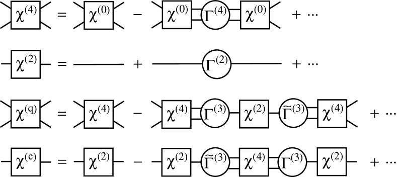
Figure 2: Diagrammatic representation of Eq. (21). Every long straight line in the second equation denotes $\hat{G}$.

$$\underline{\chi}^{({\rm q})}\equiv\left(\underline{\chi}^{(4)-1}+\underline{\Gamma}^{(3)}\hat{\chi}^{(2)}\underline{\tilde{\Gamma}}^{(3)}\right)^{\!\!-1},$$ (21c)

$$\hat{\chi}^{({\rm c})} \equiv \left(\hat{\chi}^{(2)-1}+\underline{\tilde{\Gamma}}^{(3)}\underline{\chi}^{(4)}\underline{\Gamma}^{(3)}\right)^{\!\!-1}$$ (21d)

$$= \left(\hat{G}^{-1}-\hat{\Gamma}^{(2)}+\underline{\tilde{\Gamma}}^{(3)}\underline{\chi}^{(4)}\underline{\Gamma}^{(3)}\right)^{\!\!-1},$$

where the superscripts ^q and ^c denote “quasiparticle” and “condensate,” respectively. Figure 2 expresses Eqs. (21a)-(21d) diagrammatically. Now, we can write down the solution to Eq. (20) in terms of $\underline{\chi}^{({\rm q})}$ and $\hat{\chi}^{({\rm c})}$ as

$$\delta\vec{G}=\frac{1}{2}\underline{\chi}^{({\rm q})}\bigl{(}\underline{1}+\underline{\Gamma}^{(3)}\hat{\chi}^{(2)}\underline{\tilde{\Psi}}^{(3)}\bigr{)}\delta\vec{U},$$ (22a)

$$\delta\vec{\Psi}=\frac{1}{2}\hat{\sigma}_{3}\hat{\chi}^{({\rm c})}\bigl{(}\underline{\tilde{\Psi}}^{(3)}-\underline{\tilde{\Gamma}}^{(3)}\underline{\chi}^{(4)}\bigr{)}\delta\vec{U}.$$ (22b)

Let us substitute Eq. (22) into Eq. (12b) and make use of Eq. (19) as well as $\underline{\chi}^{({\rm q})}\underline{\Gamma}^{(3)}\hat{\chi}^{(2)}=\underline{\chi}^{(4)}\underline{\Gamma}^{(3)}\hat{\chi}^{({\rm c})}$ in Eq. (21). We thereby obtain $\underline{\cal K}$ defined by Eq. (19a) as

$$\underline{\cal K} = \underline{\chi}^{({\rm q})}+\underline{\chi}^{(4)}\underline{\Gamma}^{(3)}\hat{\chi}^{({\rm c})}\underline{\tilde{\Psi}}^{(3)}+\underline{\Psi}^{(3)}\hat{\chi}^{({\rm c})}\underline{\tilde{\Gamma}}^{(3)}\underline{\chi}^{(4)}$$ (23)

$$-\underline{\Psi}^{(3)}\hat{\chi}^{({\rm c})}\underline{\tilde{\Psi}}^{(3)}.$$

This expression clearly tells us that collective modes are determined as poles of $\underline{\chi}^{({\rm q})}$ and $\hat{\chi}^{({\rm c})}$. Note in this context that poles of $\underline{\chi}^{(4)}$ in Eq. (23) are cancelled by those of $\underline{\chi}^{(4)}$ in the denominator of $\hat{\chi}^{({\rm c})}$, as seen from Eq. (21d). It also follows from Eq. (21d) that the poles of $\hat{\chi}^{({\rm c})}$ are generally not identical to those of the single-particle Green’s function $\hat{G}$ due to the additional contribution $\hat{\Gamma}^{(2)}-\underline{\tilde{\Gamma}}^{(3)}\underline{\chi}^{(4)}\underline{\Gamma}^{(3)}$, in contradiction to the statement by Gavoret and Nozières.GN64 This point will be discussed in more detail below.

Equation (23) with Eqs. (15), (19), and (21) is the main result of the present paper. The expression is formally exact, clarifies the structure of the two-particle Green’s function $\underline{\cal K}$ in terms of unambiguously defined vertices, and enables us to carry out practical calculations of $\underline{\cal K}$ for a given approximate $\Phi$ on the same footing as thermodynamic and single-particle properties. Kita09 The last point may be regarded as a definite advantage of the present formalism over the dielectric one. SK74 ; WG74 ; Griffin93

Equation (23) in the coordinate representation can be used to investigate two-particle correlations of general inhomogeneous systems, including homogeneous ones. For the latter cases, however, it is far more convenient to adopt the “energy”-momentum representation. To be specific, vertices (15) in those cases can be expanded as

$${\Gamma}^{(4)}_{ij,kl}(12,34) = \sum_{\vec{p}\vec{p}^{\,\prime}\vec{q}}{\Gamma}^{(4)}_{ij,kl}(\vec{p},\vec{p}^{\,\prime},\vec{q})\,{\rm e}^{i(\vec{p}+\vec{q})\cdot\vec{r}_{1}-i\vec{p}\cdot\vec{r}_{2}}$$ (24a)

$$\times{\rm e}^{i\vec{p}^{\,\prime}\cdot\vec{r}_{3}-i(\vec{p}^{\,\prime}+\vec{q})\cdot\vec{r}_{4}},$$

$${\Gamma}^{(3)}_{ij,k}(12,3)=\sum_{\vec{p}\vec{q}}{\Gamma}^{(3)}_{ij,k}(\vec{p},\vec{q})\,{\rm e}^{i(\vec{p}+\vec{q})\cdot\vec{r}_{1}-i\vec{p}\cdot\vec{r}_{2}-i\vec{q}\cdot\vec{r}_{3}},$$ (24b)

$$\tilde{\Gamma}^{(3)}_{i,jk}(1,23)=\sum_{\vec{p}^{\,\prime}\vec{q}}\tilde{\Gamma}^{(3)}_{i,jk}(\vec{p},\vec{q})\,{\rm e}^{i\vec{q}\cdot\vec{r}_{1}+i\vec{p}\cdot\vec{r}_{2}-i(\vec{p}+\vec{q})\cdot\vec{r}_{3}},$$ (24c)

$$\Gamma^{(2)}_{ij}(1,2)=\sum_{\vec{q}}{\Gamma}^{(2)}_{ij}(\vec{q})\,{\rm e}^{i\vec{q}\cdot(\vec{r}_{1}-\vec{r}_{2})},$$ (24d)

where $\vec{r}_{1}\equiv({\bf r}_{1},-\tau_{1})$, $\vec{p}\equiv({\bf p},\varepsilon_{n})$ with $\varepsilon_{n}\equiv 2n\pi T$ ($n=0,\pm 1,\cdots$), and the summation over $\vec{p}$ denotes $T\sum_{n}\int d^{3}p/(2\pi)^{3}$. Other quantities in Eq. (19) can be expanded similarly. The Fourier coefficients of Eqs. (19c), (19d), (19g), and (19h) are thereby obtained as

$$\chi^{(0)}_{ij,kl}(\vec{p},\vec{p}^{\,\prime},\vec{q})=\delta_{\vec{p}^{\,\prime}\vec{p}}\,G_{il}(\vec{p}+\vec{q})G_{kj}(\vec{p})+(-1)^{k+l-1}$$

$$\hskip 42.67912pt\times\delta_{\vec{p}^{\,\prime},-\vec{p}-\vec{q}}\,G_{i,3-k}(\vec{p}+\vec{q})G_{3-l,j}(\vec{p}),$$ (25a)

$$1_{ij,kl}(\vec{p},\vec{p}^{\,\prime},\vec{q})=\delta_{il}\delta_{kj}\delta_{\vec{p}^{\,\prime}\vec{p}},$$ (25b)

$$\Psi^{(3)}_{ij,k}(\vec{p},\vec{q})=(-1)^{j+k}\sqrt{n_{0}}\bigl{(}\delta_{k,3-j}\delta_{\vec{p},-\vec{q}}+\delta_{ki}\delta_{\vec{p},\vec{0}}\bigr{)},$$ (25c)

$$\tilde{\Psi}^{(3)}_{i,jk}(\vec{p},\vec{q})=(-1)^{j-1}\sqrt{n_{0}}\bigl{(}\delta_{ik}\delta_{\vec{p},\vec{0}}+\delta_{i,3-j}\delta_{\vec{p},-\vec{q}}\bigr{)},$$ (25d)

respectively, where $\delta_{\vec{p}^{\,\prime}\vec{p}}\equiv(2\pi)^{3}T^{-1}\delta({\bf p}^{\prime}-{\bf p})\delta_{n^{\prime}n}$ and $n_{0}$ denotes the condensate density. It then follows that Eqs. (21) and (23) hold as they are in terms of the Fourier coefficients. For example, Eq. (21c) can be written explicitly as an integral equation for $\chi^{({\rm q})}_{ij,kl}(\vec{p},\vec{p}^{\,\prime},\vec{q})$ as

$$\underline{\chi}^{({\rm q})}(\vec{p},\vec{p}^{\,\prime},\vec{q})=\underline{\chi}^{(4)}(\vec{p},\vec{p}^{\,\prime},\vec{q})-\sum_{\vec{p}_{1}\vec{p}_{2}}\underline{\chi}^{(4)}(\vec{p},\vec{p}_{1},\vec{q})\underline{\Gamma}^{(3)}(\vec{p}_{1},\vec{q})$$

$$\hskip 54.06023pt\times\hat{\chi}^{(2)}(\vec{q})\underline{\tilde{\Gamma}}^{(3)}(\vec{p}_{2},\vec{q})\underline{\chi}^{({\rm q})}(\vec{p}_{2},\vec{p}^{\,\prime},\vec{q}),$$ (26)

where $\underline{\chi}^{({\rm q})}$, etc., are now matrices only in terms of the Nambu indices $i,j,\cdots$, which may be defined explicitly as Eq. (19) without space-time arguments.

We now compare Eqs. (21) and (23) with the results for the two-particle Green’s function $\underline{\cal K}$ by Gavoret and Nozières. GN64 Apparently, they found the same structure for $\underline{\cal K}$ as Eq. (23) above. They subsequently identified the quantity corresponding to $\hat{\Sigma}+\hat{\Gamma}^{(2)}-\underline{\tilde{\Gamma}}^{(3)}\underline{\chi}^{(4)}\underline{\Gamma}^{(3)}$ in $\hat{\chi}^{({\rm c})}$ of Eq. (21d) with the single-particle self-energy as Eq. (3.4) of their paper, where $\tilde{M}$ and $JGGP$ on the right-hand side correspond to $\hat{\Sigma}+\hat{\Gamma}^{(2)}$ and $-\underline{\tilde{\Gamma}}^{(3)}\underline{\chi}^{(4)}\underline{\Gamma}^{(3)}$, respectively. However, they did not provide detailed reasoning to the crucial statement. In this context, we would like to point out that their analysis of $\underline{\cal K}$ was carried out separately from that of $\hat{G}$ by only investigating its diagrammatic structure in the simple perturbation expansion, where $\hat{\Gamma}^{(2)}$, for example, may be mistaken easily for a part of the single-particle self-energy, as seen from the second diagram of Fig. 2. This may be the reason why they concluded erroneously that the quantity corresponding to $\hat{\Sigma}+\hat{\Gamma}^{(2)}-\underline{\tilde{\Gamma}}^{(3)}\underline{\chi}^{(4)}\underline{\Gamma}^{(3)}$ is the single-particle self-energy. In contrast, our investigation of $\underline{\cal K}$ has been performed on the basis of Eq. (6) for $\hat{G}$ and $\vec{\Psi}$, where the self-energy $\hat{\Sigma}$ is defined unambiguously at the single-particle level. It is thereby shown that the term $\hat{\Gamma}^{(2)}-\underline{\tilde{\Gamma}}^{(3)}\underline{\chi}^{(4)}\underline{\Gamma}^{(3)}$ should be regarded as additional contribution distinct from the single-particle self-energy.

Thus, of fundamental importance will be to clarify how the extra “self-energy” $\hat{\Gamma}^{(2)}-\underline{\tilde{\Gamma}}^{(3)}\underline{\chi}^{(4)}\underline{\Gamma}^{(3)}$ in $\hat{\chi}^{({\rm c})}$ shifts its poles from those of $\hat{G}$. In the weak-coupling limit, we can show $\Gamma^{(2)}_{ii}=0$ and $\Gamma^{(2)}_{12}(1,2)=-\Gamma^{(2)*}_{21}(1,2)=-2V({\bf r}_{1}-{\bf r}_{2})\Psi({\bf r}_{1})\Psi({\bf r}_{2})$ by using Eqs. (25) and (26) of Ref. Kita09, and Eq. (15) above. Combined with $\Sigma_{12}(1,2)=V({\bf r}_{1}-{\bf r}_{2})[\Psi({\bf r}_{1})\Psi({\bf r}_{2})-\langle\phi(1)\phi(2)\rangle]$ from the lowest-order gapless $\Phi$-derivable approximation, Kita09 we thereby obtain $\Sigma_{12}(1,2)+\Gamma_{12}(1,2)=V({\bf r}_{1}-{\bf r}_{2})[-\Psi({\bf r}_{1})\Psi({\bf r}_{2})-\langle\phi(1)\phi(2)\rangle]$. Thus, at the mean-field level, $\hat{\Gamma}^{(2)}$ merely changes the sign of the condensate (i.e., dominant) contribution to the off-diagonal self-energy. It hence follows that, to the leading-order in the interaction, poles of $(\hat{G}^{-1}-\hat{\Gamma}^{(2)})^{-1}$ are the same as those of $\hat{G}$. However, they are not exactly identical due to the presence of $\langle\phi(1)\phi(2)\rangle$. Beyond the weak-coupling regime where the polarization contribution $-\underline{\tilde{\Gamma}}^{(3)}\underline{\chi}^{(4)}\underline{\Gamma}^{(3)}$ also becomes relevant in $\hat{\chi}^{({\rm c})}$, therefore, it is reasonable to expect that poles of $\hat{\chi}^{({\rm c})}$ and $\hat{G}$ are generally different. Further investigation needs to be carried out on the similarity or difference between the single-particle and collective excitations.

References

(1)M. R. Anderson, J. R. Ensher, M. R. Matthews, C. E. Wieman, and E. A. Cornell,
Science 269, 198 (1995).
(2)M. E. Peskin and D. V. Schroeder, An Introduction to Quantum Field Theory (Westview Press, Boulder, 1995).
(3)N. N. Bogoliubov, J. Phys. (USSR) 11, 23 (1947).
(4)J. Gavoret and P. Nozières, Ann. Phys.
28, 349 (1964).
(5)P. Szépfalusy and I. Kondor, Ann. Phys. 82, 1 (1974).
(6)V. K. Wong and H. Gould, Ann. Phys. 83, 252 (1974).
(7)A. Griffin, Excitations in a Bose-Condensed Liquid
(Cambridge University Press, Cambridge, 1993).
(8)P. C. Martin and J. Schwinger, Phys. Rev. 115, 1342 (1959).
(9)G. Baym and L. Kadanoff, Phys. Rev. 124, 287 (1961).
(10)G. Baym, Phys. Rev. 127, 1391 (1962).
(11)T. Kita, Prog. Theor. Phys. 123, 581 (2010).
(12)T. Kita, Phys. Rev. B 80, 214502 (2009).
(13)A. A. Abrikosov, L. P. Gorkov, and I. E. Dzyaloshinski, Methods of Quantum Field
Theory in Statistical Physics
(Prentice-Hall, Englewood Cliffs, N.J., 1963).