A large change in the predicted number of small halos due to a small amplitude oscillating inflaton potential.

Abstract

A smooth inflaton potential is generally assumed when calculating the primordial power spectrum, implicitly assuming that a very small oscillation in the inflaton potential creates a negligible change in the predicted halo mass function. We show that this is not true. We find that a small oscillating perturbation in the inflaton potential in the slow-roll regime can alter significantly the predicted number of small halos. A class of models derived from supergravity theories gives rise to inflaton potentials with a large number of steps and many transplanckian effects may generate oscillations in the primordial power spectrum. The potentials we study are the simple quadratic (chaotic inflation) potential with superimposed small oscillations for small field values. Without leaving the slow-roll regime, we find that for a wide choice of parameters, the predicted number of halos change appreciably. For the oscillations beginning in the $10^{7}-10^{8}\,\mbox{M}_{\odot}$ range, for example, we find that only a 5% change in the amplitude of the chaotic potential causes a 50% suppression of the number of halos for masses between $10^{7}-10^{8}\,\mbox{M}_{\odot}$ and an increase in the number of halos for masses $<10^{6}\,\mbox{M}_{\odot}$ by factors $\sim 15-50$. We suggest that this might be a solution to the problem of the lack of observed dwarf galaxies in the range $10^{7}-10^{8}\,\mbox{M}_{\odot}$. This might also be a solution to the reionization problem where a very large number of Population III stars in low mass halos are required.

I Introduction

Recently inflation has become an essential part of our description of the universe. Not only does it solve the classical cosmological problems of flatness, horizon and relics, but also provides precise predictions for the primordial density inhomogeneities, predictions that are in good agreement with existing observationsHinshaw et al. (2009).

Albeit these successes, the specific details of inflation are still unknown, since many different physical mechanisms and fields may generate a phase of accelerated cosmic expansion. For simplicity, it has become common practice to employ a scalar field, the inflaton, with a simple law for its potential, to generate inflation. This picture is usually understood as the effective counterpart of a deeper – and probably more complicated – theory. In this context, the most generally employed inflationary theory is the so-called chaotic inflation, characterized by a simple quadratic potential with an initial high field value for the inflaton.

Recently, due to advances in data quality and in anticipation of the data from the Planck satellite The Planck Collaboration (2006) and the Large Synoptic Survey Telescope (LSST) LSST Science Collaborations: Paul A. Abell et al. (2009)), for example, several groups started investigating more complicated forms for the inflaton potential to explain the present observational data. Pahud et al. Pahud et al. (2009) used the CMB data to look for the presence of a general sinusoidal oscillation imprinted on the inflaton potential, for large field values (i.e., large spatial dimensions), placing strong limits on the amplitude of these osillations. Ichiki et al. Ichiki and Nagata (2009) found – with a 99,995% confidence level – an oscillatory modulation for large spatial dimensions at $k\simeq 0.009\text{ Mpc}^{-1}$, performing a Monte-Carlo Markov-Chain analysis using the CMB data, confirming similar results obained from the analysis of the CMB data using different techniques Ichiki and Nagata (2009); Ichiki et al. (2009).

From a theoretical perspective, features in the inflaton potential are well motivated. Adams et al. Adams et al. (1997) showed that a class of models derived from supergravity theories gives rise to inflaton potentials with a large number of steps, each of these corresponding to a symmetry-breaking phase transition in a field coupled with the inflaton. Also, many transplanckian effects may generate oscillations in the primordial power spectrum of density inhomogeneities which could be described by an effective oscillating inflaton potential Brandenberger and Martin (2001); Martin and Brandenberger (2003).

A present major problem in astrophysics is the large discrepancy between the predicted and the observed number of dark matter halos of mass $\lesssim 10^{8}\,\mbox{M}_{\odot}$. N-body simulations designed to probe the formation and evolution of dark matter structures on small scales found $\sim 10^{3}$ dark matter halos with masses from $10^{7}\,\mbox{M}_{\odot}$ to $10^{9}\,\mbox{M}_{\odot}$ Diemand et al. (2007); Springel et al. (2008). However, very much fewer small galaxies of comparable masses are observed in the Local Group Diemand et al. (2007).

Several solutions to this number discrepancy have been proposed, ranging from selection effects in the observations Koposov et al. (2008) to complex baryonic interactions that may have swept out the baryonic gas from the small halos Macciò et al. (2010); Koposov et al. (2009). The former explanation for the discrepancy can only dimish the problem but not resolve it: taking into account the limitations of present day observations, one may extrapolate the number of dwarf galaxies to – at most – a few hundred. The latter type of solution can only be tested with semi-analytical models (for a review see Baugh (2006)), which strongly rely on the details of the physics of star formation, which is not completely understood. The ejection of gas would leave thousands of empty small dark matter halos essentially intact. There is still no clear evidence of the presence of these objects in the dynamics of the Local Group.

In this work we propose an alternative approach. Bearing in mind the growing plausability of oscillating features in the inflaton potential, we examine to what extent a simple localized oscillating modification of the inflaton potential for small field values can change the number of small dark matter halos. We restrict our analysis to perturbations of the inflaton potential which are still in the slow-roll regime.

In sections II and III we review the formalism and the derivation of the important relations used. In section IV we discuss two simple modified oscillatory potentials: a saw-tooth modification and a sinusoidal modification. In section V we present our results and in section VI our conclusions.

II Slow-roll formalism

The primordial universe is assumed to be filled by an approximately homogeneous scalar field, the inflaton, governed by a Klein-Gordon equation of motion

$$\ddot{\phi}+3H\dot{\phi}+\frac{dV}{d\phi}=0\quad\mbox{ . }$$ (1)

The Friedmann equation becomes

$$\left(\frac{\dot{a}}{a}\right)^{2}=\frac{8\pi}{3\,m_{pl}^{2}}\left[V(\phi)+\frac{1}{2}\dot{\phi}^{2}\right]\mbox{ .}$$ (2)

In order to have an inflationary period, the second derivative of the field and the kinetic term of the Friedmann equation must both be small when compared with the other terms. This can be obtained under the conditions of slow-roll,

$$\epsilon\equiv\frac{1}{8}\left(\frac{V^{\prime}(f)}{V(f)}\right)^{2}\ll 1$$ (3)

and

$$\eta\equiv\frac{1}{4}\left(\frac{V^{\prime\prime}(f)}{V(f)}\right)\ll 1\quad\mbox{,}$$ (4)

where we used the notation

$$f\equiv\frac{\sqrt{8\pi}}{m_{pl}}\phi\quad\quad\text{ and }\quad\quad V^{\prime}(f)\equiv\frac{dV}{df}\quad\text{.}$$ (5)

It is possible to associate the comoving wavenumber, $k$, of each mode of the density of perturbations with the inflaton value, $f$, when this mode was leaving the Hubble sphere. We find this using the well known (e.g. Liddle and Lyth (2000)) expression for the number of e-folds, $N(f)$,

$$\frac{k}{a_{0}H_{0}}=\exp[60-N(f)]$$ (6)

with

$$N(f)=4\int^{f}_{f_{e}}\frac{V}{V^{\prime}}\,df\approx(f^{2}-1/2)\,\,\text{ .}$$ (7)

The approximation used in Eq. (7) is justified by the fact that the assumed deviations of the chaotic inflaton potential ($V\propto f^{2}$) is very small (the interesting deviations, shown in section V are of order $5\%$).

The adimensional curvature power spectrum, $\mathcal{P}_{\mathcal{R}}$, is related to the inflaton potential, in the slow-roll approximation, by

$$\mathcal{P}_{\mathcal{R}}(k)\propto\frac{V^{3}(f(k))}{V^{\prime 2}(f(k))}\,\mbox{ ,}$$ (8)

and the normalization of the power spectrum used is the one obtained from WMAP5 Hinshaw et al. (2009).

From $\mathcal{P}_{\mathcal{R}}$ it is possible to obtain $\mathcal{P}_{\delta}$, the power spectrum of the density perturbations using (see e.g. Liddle and Lyth (2000))

$$\mathcal{P}_{\delta}(k,t)=\left[\frac{2(1+w)}{5+3w}\right]^{2}\left(\frac{k}{a(t)\,H(t)}\right)^{4}T^{2}(k)\mathcal{P}_{\mathcal{R}}$$ (9)

where $w$ is the equation of state parameter of the dominant component at instant $t$.

For the transfer function, $T(k)$, we used the analytical fit obtained by Eisenstein and Hu (1998), which takes into account the presence of dark energy and baryons.

III The mass function

The mass function gives the number density, $n(m)$ of DM halos of mass between $m$ and $m+dm$. In order to calculate it, we need first to obtain the variance from the expression

$$\sigma^{2}(R,t)=\int_{0}^{\infty}W^{2}(k,R)\mathcal{P}_{\delta}(k,t)\,\,\frac{dk}{k}$$ (10)

where we adopted a Gaussian window function

$$W^{2}(k,R)=\exp(-k^{2}R^{2})$$ (11)

In order to evaluate the mass function at the present time, we set

$$a(t)H(t)=a_{0}H_{0}=\left(2997.9\right)^{-1}h\mbox{ Mpc}^{-1}\mbox{ . }$$ (12)

Using the Press-SchechterPress and Schechter (1974) formalism, we have

$$n(m)\,dm=-\frac{\bar{\rho}}{m}\sqrt{\frac{2}{\pi}}\frac{\delta_{c}(t)}{\sigma^{2}}\frac{d\sigma}{dm}\exp\left(\frac{-\delta_{c}^{2}}{2\sigma^{2}}\right)\,dm\quad\mbox{,}$$ (13)

where $\delta_{c}\approx 1.61$ is the critical density contrast, $\bar{\rho}$ is the average density of the universe and the mass, $m$, is related with the length, $R$, from the expression

$$R(m)=\sqrt{\frac{1}{2\pi}}\left(\frac{m}{\bar{\rho}}\right)^{\frac{1}{3}}\,\mbox{ .}$$ (14)

IV Modified potentials

IV.1 Saw-tooth potentials

The modified potential to which we will refer to as ’saw-tooth’ is constructed by substituting the small field part of the quadratic potential by an oscillatory linear modification. Let $\lambda$ be the wavelength of the oscillation and $f_{a}$ the field when the modification begins. For $f>f_{a}$, $V(f)=Af^{2}$ . For $f<f_{a}$ we define $f_{n}=f_{a}-f\,n\,\lambda$.

For $f_{n}-\frac{1}{4}\lambda<f\leq f_{n}$, the potential has the form,

$$V(f)=A\frac{f_{n}^{2}-(1-b)\left(f_{n}-\frac{1}{4}\lambda\right)^{2}}{\frac{1}{4}\lambda}+Af_{n}^{2}\,\text{ , }$$ (15)

for $f_{n}-\frac{1}{2}<f\leq f_{n}-\frac{1}{4}\lambda$,

$$V(f)=A\frac{(1-b)\left(f_{n}-\frac{1}{4}\lambda\right)^{2}-\left(f_{n}-\frac{1}{2}\lambda\right)^{2}}{\frac{1}{4}\lambda}\left(f-f_{n}+\frac{1}{4}\lambda\right)+A(1-b)\left(f_{n}-\frac{1}{4}\lambda\right)^{2}\text{ , }$$ (16)

for $f_{n}-\frac{3}{4}<f\leq f_{n}-\frac{1}{2}\lambda$,

$$V(f)=A\frac{\left(f_{n}-\frac{1}{2}\lambda\right)^{2}-(1+b)\left(f_{n}-\frac{3}{4}\lambda\right)^{2}}{\frac{1}{4}\lambda}\left(f-f_{n}+\frac{1}{2}\lambda\right)+A\left(f_{n}-\frac{1}{2}\lambda\right)^{2}\text{ ,}$$ (17)

and for $f_{n+1}<f\leq f_{n}-\frac{3}{4}\lambda$,

$$V(f)=A\frac{(1+b)\left(f_{n}-\frac{1}{4}\lambda\right)^{2}-\left(f_{n}-\frac{1}{2}\lambda\right)^{2}}{\frac{1}{4}\lambda}\left(f-f_{n}+\frac{1}{4}\lambda\right)+A(1+b)\left(f_{n}-\frac{1}{4}\lambda\right)^{2}\text{ .}$$ (18)

The potential is shown in Fig. 1.

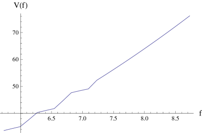
Figure 1: Saw-tooth potential, with $b=0.025$ and $\lambda=0.55$

In Fig. 1 we take $f_{a}=7.232$ in order to obtain changes in the variance for mass scales $M\lesssim 10^{8}\,\mbox{M}_{\odot}$. We are in the parameter space region of slow-roll inflation. The part of the parameter space which allows for this regime – i.e., where the slow-roll parameters (Eq. (3) and Eq. (4)) are smaller than 1 – is shown in Fig. 2.

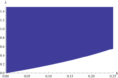
Figure 2: The shaded area indicates the region of the parameter space, $(\lambda,b)$, where the saw-tooth potential is compatible with slow-roll inflation.

IV.2 Sinusoidal potentials

We also analyse the case when the modification of the potential is a simple sine wave,

$$V(f)=\left\{\begin{array}[]{l}Af^{2}\left[1+b\sin\left(\frac{2\pi\,f}{\lambda}\right)\right]\,\text{ , }\,f\leq f_{a}\\ Af^{2}\mbox{ , }f>f_{a}\\ \end{array}\right.\quad\mbox{,}$$ (19)

which is plotted in Fig. 3.

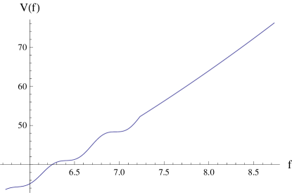
Figure 3: Sinusoidal potential, with $b=0.025$ and $\lambda=0.55$

The parameter $f_{a}$ was chosen using the same criterion as in the saw-tooth case. We tested again for the area of the parameter space which was compatible with the slow-roll regime which is shown in Fig. 4.

Figure 4: The shaded area indicates the region of the parameter space, $(\lambda,b)$, where the sinusoidal potential is compatible with slow-roll inflation.

V Results

We calculated the dimensional density perturbation power spectrum ($P(k)=2\pi^{2}\mathcal{P}_{\delta}(k)/k^{3}$, following Eq. (9), which is shown, for representative parameter values, in Fig. 5.

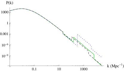
Figure 5: Power spectrum obtained using a saw-tooth potential with different values of $b$ and $\lambda$. The continuous (green) curve corresponds to $b=0.025$ and $\lambda=0.55$; the dotted (blue) curve, to $b=0.050$ and $\lambda=0.75$, and the dashed (black) curve, to $b=0.015$ and $\lambda=0.45$.

The same quantity was calculated for the sinusoidal potential, as shown in Fig.6.

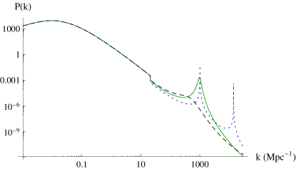
Figure 6: Power spectrum obtained using a sinusoidal potential with different values of $b$ and $\lambda$. The continuous (green) curve corresponds to $b=0.025$ and $\lambda=0.55$; the dotted (blue) curve, to $b=0.050$ and $\lambda=0.75$, and the dashed (black) curve, to $b=0.015$ and $\lambda=0.45$.

In Fig. 7 we plot the ratio of the mass function obtained from the saw-tooth potential to the mass function of a featureless quadratic potential (i.e., ${n_{saw-tooth}(m)}/{n_{ch}(m)}$ ), for different values of the parameters $b$ and $\lambda$, with $b$ varying from 1.5% to 5%.

When using parameters $b=0.05$ (i.e., a 5% modification of the chaotic potential) and $\lambda=0.75$, we find a $47\%$ suppression in the number of halos for masses between $10^{7}$ and $10^{8}\,\mbox{M}_{\odot}$.

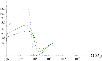
Figure 7: Ratio $r=n_{\text{saw-tooth}}(m)/n_{\text{chaotic}}(m)$ . The continuous (green) curve corresponds to $b=0.025$ and $\lambda=0.55$; the dotted (blue) curve, to $b=0.050$ and $\lambda=0.75$, and the dashed (black) curve, to $b=0.015$ and $\lambda=0.45$.

In Fig. 8 we plot the ratio of the mass function obtained from the sinusoidal potential to the mass function of a featureless quadratic potential, again for different values of the parameters $b$ and $\lambda$. Using parameters $b=0.05$ and $\lambda=0.75$, we find a $54\%$ suppression in the number of halos for masses between $10^{7}$ and $10^{8}\,\mbox{M}_{\odot}$.

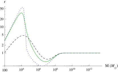
Figure 8: Ratio $r=n_{\text{sin}}(m)/n_{\text{chaotic}}(m)$ . The continuous (green) curve corresponds to $b=0.025$ and $\lambda=0.55$; the dotted (blue) curve, to $b=0.050$ and $\lambda=0.75$, and the dashed (black) curve, to $b=0.015$ and $\lambda=0.45$.

VI Conclusions

We modified the inflationary potential introducing two kinds of oscillatory patterns superimposed, for small field values, on a quadratic potential. Our modifications are small enough to be compatible with the slow roll conditions and consequently do not alter the usual and successful inflationary predictions for the large scale regime.

The first modification studied (Eq.s (15)-(18)) has the form of a succession of linear segments that creates an oscillating saw-tooth pattern which deviates from the standard quadratic potential by a factor $b$. Using the Press-Schechter formalism, we found that the number of small mass halos can be strongly reduced for many choices of the parameters $b$ (which characterizes the amplitude) and $\lambda$ (which characterizes the wavelength). For example, we found that the number of halos with masses between $10^{7}$ and $10^{8}\,\mbox{M}_{\odot}$ decreases by 47% for $b=0.05$ and $\lambda=0.75$.

The second modification studied (Eq. (19)) is a simple sine function multiplying the quadratic potential. This modification allows one to capture the effects of the previous one without the discontinuities in the second derivatives. Once again we calculated the mass function using the Press-Schechter formalism and found a strong suppression in the number of small halos for a wide area of the parameter space. As a representative example, we found that the number of halos with masses between $10^{7}$ and $10^{8}\,\mbox{M}_{\odot}$ decreases by 54% for $b=0.05$ and $\lambda=0.75$.

We conclude that small oscillatory patterns on the inflaton potential can cause large changes in the predicted halo mass function. In particular, if the oscillations begin in the $10^{7}-10^{8}\,\mbox{M}_{\odot}$ range, for example, the oscillations can appreciably suppress the number of dwarf galaxies in this mass range, as observed. It also appreciably increases the number of halos of mass $<10^{6}\,\mbox{M}_{\odot}$ by factors $\sim 15-60$. This might be a solution to the reionization problem where a very large number of Population III stars in low mass halos are required.

Although we found that a small amplitude ($b=5\%$) saw-tooth oscillatory inflaton potential, with a “wavelength” $\lambda=0.75$, causes a factor of $\sim 2$ decrease in the number of halos of masses $10^{7}-10^{8}\,\mbox{M}_{\odot}$, present observations indicate a much larger depression – although the upper limit of the number of observed dwarf galaxies is not well defined due to observational difficulties. From our Fig. 2, however, $\lambda$ could be much less than 0.75 with $b=5\%$, in particular, $\lambda$ could be as small as $\lambda\sim 0.1$, and still be compatible with slow-roll inflation. A detailed analysis of the parameter space $(\lambda,b)$, as well as more general inflation models than the simple single scalar chaotic inflation model which was used here, is thus required (which is now in progress). Only then can we know whether a small amplitude oscillatory inflaton potential, alone, can resolve the problem of the lack of observed dwarf galaxies in the range $10^{7}-10^{8}\,\mbox{M}_{\odot}$.

References

- Hinshaw et al. (2009) G. Hinshaw, J. L. Weiland, R. S. Hill, N. Odegard, D. Larson, C. L. Bennett, J. Dunkley, B. Gold, M. R. Greason, N. Jarosik, et al., The Astrophysical Journals 180, 225 (2009), eprint arXiv:0803.0732.
- The Planck Collaboration (2006) The Planck Collaboration, ArXiv Astrophysics e-prints (2006), eprint arXiv:astro-ph/0604069.
- LSST Science Collaborations: Paul A. Abell et al. (2009) LSST Science Collaborations: Paul A. Abell, J. Allison, S. F. Anderson, J. R. Andrew, J. R. P. Angel, L. Armus, D. Arnett, S. J. Asztalos, T. S. Axelrod, S. Bailey, et al., ArXiv e-prints (2009), eprint arXiv:0912.0201.
- Pahud et al. (2009) C. Pahud, M. Kamionkowski, and A. R. Liddle, Physical Review D 79, 083503 (2009), eprint arXiv:0807.0322.
- Ichiki and Nagata (2009) K. Ichiki and R. Nagata, Physical Review D 80, 083002 (2009).
- Ichiki et al. (2009) K. Ichiki, R. Nagata, and J. Yokoyama, ArXiv e-prints (2009), eprint arXiv:0911.5108.
- Adams et al. (1997) J. A. Adams, G. G. Ross, and S. Sarkar, Nuclear Physics B 503, 405 (1997), eprint arXiv:hep-ph/9704286.
- Brandenberger and Martin (2001) R. H. Brandenberger and J. Martin, Modern Physics Letters A 16, 999 (2001), eprint arXiv:astro-ph/0005432.
- Martin and Brandenberger (2003) J. Martin and R. Brandenberger, Physical Review D 68, 063513 (2003), eprint arXiv:hep-th/0305161.
- Diemand et al. (2007) J. Diemand, M. Kuhlen, and P. Madau, The Astrophysical Journal 657, 262 (2007), eprint arXiv:astro-ph/0611370.
- Springel et al. (2008) V. Springel, J. Wang, M. Vogelsberger, A. Ludlow, A. Jenkins, A. Helmi, J. F. Navarro, C. S. Frenk, and S. D. M. White, Monthly Notices of the Royal Astronomical Society 391, 1685 (2008), eprint arXiv:0809.0898.
- Koposov et al. (2008) S. Koposov, V. Belokurov, N. W. Evans, P. C. Hewett, M. J. Irwin, G. Gilmore, D. B. Zucker, H. Rix, M. Fellhauer, E. F. Bell, et al., The Astrophysical Journal 686, 279 (2008), eprint arXiv:0706.2687.
- Macciò et al. (2010) A. V. Macciò, X. Kang, F. Fontanot, R. S. Somerville, S. Koposov, and P. Monaco, Monthly Notices of the Royal Astronomical Society 402, 1995 (2010), eprint arXiv:0903.4681.
- Koposov et al. (2009) S. E. Koposov, J. Yoo, H. Rix, D. H. Weinberg, A. V. Macciò, and J. M. Escudé, The Astrophysical Journal 696, 2179 (2009), eprint arXiv:0901.2116.
- Baugh (2006) C. M. Baugh, Reports on Progress in Physics 69, 3101 (2006), eprint arXiv:astro-ph/0610031.
- Liddle and Lyth (2000) A. R. Liddle and D. H. Lyth, Cosmological Inflation and Large-Scale Structure (2000).
- Eisenstein and Hu (1998) D. J. Eisenstein and W. Hu, The Astrophysical Journal 496, 605 (1998), eprint arXiv:astro-ph/9709112.
- Press and Schechter (1974) W. H. Press and P. Schechter, The Astrophysical Journal 187, 425 (1974).