Hidden $Sp(2s\!+\!1)$- or $SO(2s\!+\!1)$-symmetry and new exactly solvable models
in ultracold atomic systems

Yuzhu Jiang Beijing National Laboratory for Condensed Matter Physics, Institute of Physics, Chinese Academy of Sciences, Beijing 100190, People’s Republic of China Technical Institute of Physics and Chemistry, Chinese Academy of Sciences, Beijing 100190, People’s Republic of China    Junpeng Cao Beijing National Laboratory for Condensed Matter Physics, Institute of Physics, Chinese Academy of Sciences, Beijing 100190, People’s Republic of China    Yupeng Wang Beijing National Laboratory for Condensed Matter Physics, Institute of Physics, Chinese Academy of Sciences, Beijing 100190, People’s Republic of China
Abstract

The high spin ultracold atom models with a special form of contact interactions, i.e., the scattering lengthes in the total spin-$2,4\cdots$ channels are equal but may be different from that in the spin-0 channel, is studied. It is found that those models have either $Sp(2s+1)$-symmetry for the fermions or $SO(2s+1)$-symmetry for the bosons in the spin sector. Based on the symmetry analysis, a new class of exactly solvable models is proposed and solved via the Bethe ansatz. The ground states for repulsive fermions are also discussed.

Sp(2s+1), SO(2s+1), multipole, quantum gas, exact solutions
pacs:
02.30.Ik 03.75.Mn 67.85.Bc

I Introduction

Recently, the study on cold atoms with high spin has aroused lots of attention in the fields of atomic, molecular, optical and condensed matter physics. Due to the spin exchange interactions, many interesting spin ordered states arise and the phase diagrams of these systems are very rich. For instance, in the spin-1 spinor Bose–Einstein condensations, the bosons are found to form the pairs and the pairs condense even in the repulsive regime Law1998PRL ; Mukerjee2006PRL ; Mueller2006PRA . In experiments, by using the atom cooling and trapping techniques, one can prepare the high spin cold atomic systems, such as 7Li Bradley1995PRL , 23Na Stamper-Kurn1998PRL1 , 87Rb Myatt1997PRL ; Barrett2001PRL ; Paredes2004N with hyperfine spin 1; 53Cr Chicireanu2006PRA with hyperfine spin 3/2; and 40K DeMarco1999S , 173Yb Takasu2006LP , 43Ca Witte1992JOSAB , 87Sr Xu2003JOSAB , 133Cs Soding1998PRL ; Ma2004JPB with more higher ones. Using the Feshbach resonance Inouye1998N ; Dickerscheid2005PRA and confinement induced resonance Bergeman2003PRL technique, the interactions among the atoms can be manipulated. This provides a good platform for studying the tunable condensed matter systems. In theoretical approaches, the low-energy effective models of the dilute ultracold atomic systems are the quantum gas with contact interactions, and the spin exchanging interactions should also be considered for systems with internal degrees of freedom Ho1998PRL ; Ohmi1998JPSJ .

Symmetric analysis plays a very important role in studying the quantum many-body systems. Physical properties such as ground state manifold and order parameters are closely related to the symmetry of a system WuCJ2005PRL ; ChenS2005PRB ; WuCJ2006MPLB . The analysis of the symmetry can give us some hints to do the suitable approximation and study the physics such as phase diagram in the frame of mean-field theory. It can also simplify the analytical and numerical calculations. In the cold atomic systems with delta function interactions, the symmetric or anti-symmetric properties of the identical particles restrict the forms of spin exchange interactions. Effective spin exchanging interactions only take place in the channels with symmetric spatial wave function. Such property may make the systems to have intrinsic symmetries in the spin sector. For example, in the spin-$3/2$ system, the $SO(5)$ symmetry is found WuCJ2003PRL .

The strong quantum fluctuation and correlation make the physics of one-dimensional (1D) system quite different from the ones of higher dimensions. Many numerical and analytical methods are developed to study the 1D systems. The exact solution is a good starting point to study these systems, since it can give us conclusive results. A well-known exactly solvable system in the cold atomic system is the Lieb–Liniger model LiebLiniger1963PR , where the scalar bosons are studied. The fermion case with spin-1/2 are exactly solved by Yang Yang1967PRL . Sutherland generalized Yang’s model to arbitrary spin case, where the system has the $SU(2s+1)$ symmetry Sutherland1968PRL , with $s$ the spin of the particles. At present, it is clear that the multicomponent quantum gas including the Bose–Fermi mixtures with delta function interactions are integrable, if the masses of each species are equal and the interactions are equal Zhou1988JPA1 ; Lai1971PRA ; Pu1987JPA . In these models, the scattering lengthes in different channels are the same, for that the spin exchange interactions are not considered. However, the spin exchanging usually can not be neglected in experiments, and many novel ordered states are induced by the spin exchanging. Motivated by this consideration, we proposed a $SO(3)$ integrable spin-1 bosonic model Cao2007EPL and a $Sp(4)$ integrable spin-3/2 fermionic model Jiang2009EPL , where the contact spin exchange interactions are considered. The scattering lengthes in different channels are different.

This paper is a generalization of our previous works Cao2007EPL ; Jiang2009EPL to cold atom systems with arbitrary hyperfine spins. For a special interaction form of atoms with hyperfine spin $s$, we find that the fermion system has the $U(1)\otimes Sp(2s+1)$ symmetry while the boson system has the $U(1)\otimes SO(2s+1)$ symmetry. The generators of corresponding algebra are constructed by the magnetic multipole operators. Based on the symmetry analysis, we propose a new class of exactly solvable models in one dimension.

II Model and symmetry

For the delta function interaction models of dilute cold atomic gas with hyperfine spin $s$, the spin exchange interaction between two particles $i$ and $j$ is usually written as spin projection operators $\hat{P}^{l}_{ij}$ in different channels with total spin-$l$ ($l=0,1,2,\cdots,2s$). Nontrivial scattering processes occur only in the even $l$ channels because of the symmetry or anti-symmetry behavior of the wave functions. To study the behavior of such systems away from the $SU(2s+1)$ symmetry point, we consider a simple case, i.e., all the scattering lengths of nonzero $l$ channels are the same. The Hamiltonian reads

H^=βˆ’βˆ‘i=1Nβˆ‡π’“j2+βˆ‘iβ‰ jN[c1​P^i​j0+c2β€‹βˆ‘l=2,4,β‹―P^i​jl]​δ​(𝒓iβˆ’π’“j).^𝐻superscriptsubscript𝑖1𝑁subscriptsuperscriptβˆ‡2subscript𝒓𝑗superscriptsubscript𝑖𝑗𝑁delimited-[]subscript𝑐1subscriptsuperscript^𝑃0𝑖𝑗subscript𝑐2subscript𝑙24β‹―subscriptsuperscript^𝑃𝑙𝑖𝑗𝛿subscript𝒓𝑖subscript𝒓𝑗\hat{H}=-\sum_{i=1}^{N}\nabla^{2}_{{\boldsymbol{r}}_{j}}+\sum_{i\neq j}^{N}\Big{[}c_{1}\hat{P}^{0}_{ij}+c_{2}\!\!\sum_{l=2,4,\cdots}\!\!\hat{P}^{l}_{ij}\Big{]}\delta({\boldsymbol{r}}_{i}-{\boldsymbol{r}}_{j}). (1)

Here, $N$ is the number of atoms, ${\boldsymbol{r}}_{i}$ is the position of the $i$-th atom, $c_{1}$ is the interaction strength in spin-0 channel and $c_{2}$ is the one in other channels.

Refer to caption
Figure 1: The sketches of two-atom scattering processes.

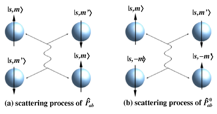
The two-body scattering in the system (1) is quite interesting. There are two kinds of scattering processes in the spin sector. One is |s,m;s,mβ€²βŸ©β€‹βŸ¨s,mβ€²;s,m|+h.c.formulae-sequenceketπ‘ π‘šπ‘ superscriptπ‘šβ€²bra𝑠superscriptπ‘šβ€²π‘ π‘šβ„Žπ‘|s,m;s,m^{\prime}\rangle\langle s,m^{\prime};s,m|+h.c. provided by two-particle permutation as shown in Fig. 1(a), here $m$ and $m^{\prime}$ are the spins along $z$ direction, and m,mβ€²=s,sβˆ’1,β‹―,βˆ’sformulae-sequenceπ‘šsuperscriptπ‘šβ€²π‘ π‘ 1⋯𝑠m,m^{\prime}=s,s-1,\cdots,-s. In this process, the particle numbers $\hat{N}_{m}$ with different $m$ are invariant. As a consequence, the total spin $\hat{\boldsymbol{S}}$ and total particle number $\hat{N}$ are also conserved. The other scattering process is |s,m;s,βˆ’mβŸ©β€‹βŸ¨s,mβ€²;s,βˆ’mβ€²|+h.c.formulae-sequenceketπ‘ π‘šπ‘ π‘šbra𝑠superscriptπ‘šβ€²π‘ superscriptπ‘šβ€²β„Žπ‘|s,m;s,-m\rangle\langle s,m^{\prime};s,-m^{\prime}|+h.c. provided by the projector operator $\hat{P}^{0}_{ab}$, as shown in Fig. 1(b). In this process, two particles with opposite spins scatter into another pair, and the absolute value $|m^{\prime}|$ can be unequal to $|m|$. Obviously, this process does not affect the total particle number $\hat{N}$, but it destroys the invariability of $\hat{N}_{m}$. Therefore, the particle number $\hat{N}_{m}$ no longer conserves. Nevertheless, by careful consideration, we find that $\hat{J}_{m}=\hat{N}_{m}-\hat{N}_{-m}$ with m=s,sβˆ’1,β‹―π‘šπ‘ π‘ 1β‹―m=s,s-1,\cdots and $m\geq 0$ are still invariant. The invariance of $J_{m}$ means that the total spin $\hat{S}=\sum_{m}m\hat{J}_{m}$ is still a good quantum number. Besides, some of the magnetic multipole operators are also invariant. The multipole operators are observable physical quantities and can be defined in the form of irreducible tensors,

T^ml=(l+m)!​(lβˆ’m)!/(2​l)!​(∏j=1lβˆ’1βˆ‘mjs~^mjβ€²)​s~^mβˆ’βˆ‘i=1lβˆ’1mi,m=βˆ’l,βˆ’l+1,β‹―,l,l=1,2,β‹―,2​s,s~^βˆ’1=(s^xβˆ’i​s^y)/2,s~^0=2​s^z,S~^1=βˆ’(s^x+i​s^y)/2.formulae-sequencesubscriptsuperscript^π‘‡π‘™π‘šπ‘™π‘šπ‘™π‘š2𝑙superscriptsubscriptproduct𝑗1𝑙1subscriptsubscriptπ‘šπ‘—superscriptsubscript^~𝑠subscriptπ‘šπ‘—β€²subscript^~π‘ π‘šsuperscriptsubscript𝑖1𝑙1subscriptπ‘šπ‘–formulae-sequenceπ‘šπ‘™π‘™1⋯𝑙formulae-sequence𝑙12β‹―2𝑠formulae-sequencesubscript^~𝑠1superscript^𝑠π‘₯isuperscript^𝑠𝑦2formulae-sequencesubscript^~𝑠02superscript^𝑠𝑧subscript^~𝑆1superscript^𝑠π‘₯isuperscript^𝑠𝑦2\begin{split}&\hat{T}^{l}_{m}\!=\!\sqrt{\!{{(l\!+\!m)!(l\!-\!m)!}}/\!{{(2l)!}}}\Big{(}\!\prod_{j=1}^{l-1}\sum_{m_{j}}~\!{}^{{}^{\!\!{}^{\prime}}}\!\hat{\tilde{s}}_{m_{j}}\!\Big{)}\!\hat{\tilde{s}}_{m\!-\!\sum_{i=1}^{l-1}m_{i}},\\ &\hskip 53.0ptm=-l,-l+1,\cdots,l,~{}~{}l=1,2,\cdots,2s,\\ &\hat{\tilde{s}}_{-1}\!=\!(\hat{s}^{x}\!\!-\!{\rm i}\hat{s}^{y})/\sqrt{2},~{}\hat{\tilde{s}}_{0}\!=\!{\sqrt{2}}\hat{s}^{z},~{}\hat{\tilde{S}}_{1}\!=\!-(\hat{s}^{x}\!\!+\!{\rm i}\hat{s}^{y})/\sqrt{2}.\end{split} (2)

Here, $\hat{s}^{\alpha}$ ($\alpha=x,y,z$) is the spin operators of one particle, $m_{j}=-1,0,1$, and the sum $\Sigma^{\prime}$ means $|m-\sum_{i}^{j}m_{i}|<l-j$ for any $j$. The total multipole operators for $N$ particles are $\hat{M}^{l}_{m}=\sum_{i=1}^{N}\hat{T}^{i,l}_{m}$, where $\hat{T}^{i,l}_{m}$ is the $l$-rank multipole operator of the $i$-th particle. It can be proved that the multipole operators with odd rank are commutative with the Hamiltonian

$\displaystyle[\hat{V},\hat{M}^{l}_{m}]=0,$ (3)

where V^=βˆ‘iβ‰ jN(c1​P^i​j0+c2β€‹βˆ‘l=2,4,β‹―P^i​jl)^𝑉superscriptsubscript𝑖𝑗𝑁subscript𝑐1subscriptsuperscript^𝑃0𝑖𝑗subscript𝑐2subscript𝑙24β‹―subscriptsuperscript^𝑃𝑙𝑖𝑗\hat{V}=\sum_{i\neq j}^{N}(c_{1}\hat{P}^{0}_{ij}+c_{2}\sum_{l=2,4,\cdots}\hat{P}^{l}_{ij}), and thus are the conserved quantities of system (1). This can be understood from the two-body scattering processes. If we only consider the process of permutation, all multipole operators are commutative with the spin part of the Hamiltonian, since the exchanges of spins have no effect on the magnetic properties. However, the scattering processes of $\hat{P}^{0}_{ab}$ make the magnetic quadrupole change.

The odd rank multipole operators can be used to construct the generators of $Sp(2s+1)$ (half odd $s$) and $SO(2s+1)$ (integer $s$) algebras. Because the algebras $\mathfrak{so}(s,s+1)$ and $\mathfrak{so}(2s+1)$ have the same complex extensions $\mathfrak{so}(2s+1,\mathds{C})$, and if a model possesses the $SO(s,s+1)$ symmetry, it must have the $SO(2s+1)$ symmetry. Here we use group $SO(s,s+1)$ instead of $SO(2s+1)$ to reveal the hidden symmetry in the system (1). The generators of these groups can be defined uniformly as the $(2s+1)\times(2s+1)$ matrices satisfying the following conditions

$\displaystyle\!\!\!{\rm tr}\hat{Y}=0,~{}\hat{Y}=-\hat{Y}^{*},~{}\hat{Y}^{t}\hat{J}+\hat{J}\hat{Y}=0.$ (4)

Although the operator $\hat{J}$ is different for $Sp(2s+1)$ and $SO(s,s+1)$ groups, we can write it in a uniform representation

Jmβ€²m=(βˆ’1)sβˆ’m′​δm,βˆ’mβ€²,m,mβ€²=s,sβˆ’1,β‹―,βˆ’s.formulae-sequencesubscriptsuperscriptπ½π‘šsuperscriptπ‘šβ€²superscript1𝑠superscriptπ‘šβ€²subscriptπ›Ώπ‘šsuperscriptπ‘šβ€²π‘šsuperscriptπ‘šβ€²π‘ π‘ 1⋯𝑠\displaystyle J^{m}_{m^{\prime}}=(-1)^{s-m^{\prime}}\delta_{m,-m^{\prime}},~{}m,m^{\prime}=s,s-1,\cdots,-s. (5)

Note that it is not valid for $SO(s,s+1)$ group with half odd $s$, and we use $SO(s,s+1)$ group for the ones with integer $s$ ($B_{n}$ type algebra, $n=s$) in the following discussions.

Eq. (5) shows a similarity of $Sp(2s+1)$ and $SO(s,s+1)$ groups. This enables the different symmetries of Hamiltonian (1) to be proven simultaneously. Since the multipole operators defined in eq. (2) are all $(2s+1)^{2}-1$ linearly independent $(2s+1)\times(2s+1)$ real matrices with zero trace, we can use them to construct the generators of $Sp(2s+1)$ and $SO(s,s+1)$ group. If we choose the basis of multipole operators (2) as the eigenstates of $\hat{s}^{z}$ and the representation of $\hat{J}$ takes the form of (5), the generators of $Sp(2s+1)$ and $SO(s,s+1)$ groups defined in (4) can be represented as

$\displaystyle\hat{Y}^{l}_{m}={\rm i}\hat{T}^{j}_{m},\mbox{(odd $l$)}.$ (6)

Therefore, $(s+1)(2s+1)$ operators $\hat{Y}^{l}_{m}$ are the generators of $Sp(2s+1)$ group if $s$ is half odd, and the $s(2s+1)$ operators $\hat{Y}^{l}_{m}$ are the generators of $SO(s,s+1)$ group if $s$ is integer. For that multipole operators with odd rank-$l$ are commutative with the spin part of Hamiltonian, eq. (3), the corresponding symmetries hold for the system (1). There is also a $U(1)$ symmetry for the coordinate part, then the system (1) has $U(1)\otimes Sp(2s+1)$ symmetry for the fermionic case and $U(1)\otimes SO(2s+1)$ symmetry for the bosonic case.

There are three homomorphisms $Sp(2)\simeq SU(2)$, $SO(3)\simeq SU(2)$ and $Sp(4)\simeq SO(5)$. For the case $s=1/2$, only one channel $\hat{P}^{0}_{ab}$ involved, the model in the spin sector has the $SU(2)$ ($Sp(2)$) symmetry. For the cases $s=1$ and $3/2$, two channels $\hat{P}^{0}_{ab}$ and $\hat{P}^{2}_{ab}$ are involved. When $s=1$, the model has $SU(2)$ ($SO(3)$) symmetry, and when $s=3/2$ the system has $SO(5)$ ($Sp(4)$) symmetry, which are consistent with the results obtained in the references WuCJ2003PRL .

When $c_{1}=c_{2}$, the symmetry of the system (1) in the spin sector degenerates into the $SU(2s+1)$ one, where all the interaction strengthes in different channels are the same. The interaction of the spin part is the spin permutation operator up to a constant. The permutation operator acting on the symmetric wave functions gives the eigenvalue 1, and the one acting on the anti-symmetric wave functions gives $-1$. Thus the effective interaction is just the contact interaction and all magnetic multipoles are conserved. This can also be explained from the view that only the permutation operators are involved in the scattering process. In the form of multipole operators, the $(2s+1)^{2}-1$ generators of $SU(2s+1)$ group read Y^j​ms=im​(T^mj+T^βˆ’mj)/2subscriptsuperscript^π‘Œπ‘ π‘—π‘šsuperscriptiπ‘šsubscriptsuperscript^π‘‡π‘—π‘šsubscriptsuperscript^π‘‡π‘—π‘š2\hat{Y}^{s}_{jm}\!=\!{\rm i}^{m}(\hat{T}^{j}_{m}\!+\!\hat{T}^{j}_{\!-m})/2 and $\hat{Y}^{a}_{jm}\!=\!{\rm i}^{m+1}(\hat{T}^{j}_{m}\!-\!\hat{T}^{j}_{\!-m})\!/2$.

III Exactly solvable models

In one dimension, it is well-known that at the $SU(2s+1)$ symmetry point, the model is integrable. As we showed in the spin-1 Cao2007EPL and spin-3/2 Jiang2009EPL cases, there is indeed another integrable point. For the $Sp(2s+1)$ or $SO(2s+1)$-invariant Hamiltonian (1), we construct the following exactly solve model by constricting the parameters $c_{0}$ and $c_{2}$:

H^int=βˆ’βˆ‘i=1Nβˆ‚2βˆ‚xi2+βˆ‘iβ‰ jNV^i​jint​δ​(xiβˆ’xj),V^i​jint=(βˆ’1)2​s+1​[s+12βˆ’(βˆ’1)2​s]​c​P^i​j0+cβ€‹βˆ‘l=2,4,β‹―P^i​jl.formulae-sequencesuperscript^𝐻intsuperscriptsubscript𝑖1𝑁superscript2superscriptsubscriptπ‘₯𝑖2superscriptsubscript𝑖𝑗𝑁subscriptsuperscript^𝑉int𝑖𝑗𝛿subscriptπ‘₯𝑖subscriptπ‘₯𝑗subscriptsuperscript^𝑉int𝑖𝑗superscript12𝑠1delimited-[]𝑠12superscript12𝑠𝑐subscriptsuperscript^𝑃0𝑖𝑗𝑐subscript𝑙24β‹―subscriptsuperscript^𝑃𝑙𝑖𝑗\begin{split}&\hat{H}^{\rm int}=-\sum_{i=1}^{N}\frac{\partial^{2}}{\partial{x}_{i}^{2}}+\sum_{i\neq j}^{N}\hat{V}^{\rm int}_{ij}\delta({x}_{i}-{x}_{j}),\\ &\hat{V}^{\rm int}_{ij}=(-1)^{2s+1}\big{[}s+\frac{1}{2}-(-1)^{2s}\big{]}c\hat{P}^{0}_{ij}+c\!\!\!\sum_{l=2,4,\cdots}\!\!\!\hat{P}^{l}_{ij}.\end{split} (7)

With standard coordinate Bethe ansatz method, the wave function of the system (7) is assumed as

$\displaystyle\varPsi_{\!E}\!=\!\sum_{\mathcal{QP}}\!\Theta(x_{\!{\mathcal{Q}}_{1}}\!<\!\cdots\!<\!x_{\!{\mathcal{Q}}_{N}})A_{m_{1}\!,\cdots,m_{N}}\!(\!\mathcal{Q},\!\mathcal{P}){\rm e}^{{\rm i}\!\sum_{n}\!x_{\mathcal{Q}_{n}}k_{\mathcal{P}_{n}}}\!.\!\!\!\!$ (8)

Here, $m_{i}$ is the spin component along $z$-direction of $i$-th particle, mi=s,sβˆ’1,β‹―,βˆ’ssubscriptπ‘šπ‘–π‘ π‘ 1⋯𝑠m_{i}=s,s-1,\cdots,-s, and $k_{i}$ ($i=1,2,\cdots,N$) are the quasi-momenta carried by the particles. ${\mathcal{Q}}$ and ${\mathcal{P}}$ are all $N!$ permutations of $\{1,2,\cdots,N\}$, and ${\mathcal{Q}}_{i}$ ( ${\mathcal{P}}_{i}$) is the $i$-th number of the permutation ${\mathcal{Q}}$ (${\mathcal{P}}$). $\Theta(x_{{\mathcal{Q}}_{1}}\!<\!\cdots\!<\!x_{{\mathcal{Q}}_{N}})\!=\!\prod_{i=2}^{N}\theta(x_{{\mathcal{Q}}_{i}}\!-\!x_{{\mathcal{Q}}_{i-1}})$ is continuous multiplication of step function $\theta(x)$. When $x\geq 0$, $\theta(x)=1$, and otherwise $\theta(x)=0$. Thus the function $\Theta$ divides the coordinate space into $N!$ intervals.

The two-particle scattering occurs at the interface of two adjacent coordinate intervals ${\cal Q}$ and ${\cal Q^{\prime}}$. The scattering matrix of particles $a$ and $b$ carrying different quasi-momenta is defined in the two-particle spin space to describe the relation of the superposition coefficients

$\displaystyle\vec{A}({\mathcal{Q}},{\mathcal{P}})=\hat{S}_{{}^{{\mathcal{Q}}_{\xi},{\mathcal{Q}}_{\xi+1}}}(k_{{}^{{\mathcal{P}}_{\xi+1}}}\!\!-\!k_{{}^{{\mathcal{P}}_{\xi}}})\vec{A}({\mathcal{Q}}^{\prime},{\mathcal{P}}^{\prime}),$ (9)
$\displaystyle{\mathcal{Q}}^{\prime}=\{{\mathcal{Q}}_{1},{\mathcal{Q}}_{2},\cdots,{\mathcal{Q}}_{\xi-1},{\mathcal{Q}}_{\xi+1},{\mathcal{Q}}_{\xi},{\mathcal{Q}}_{\xi+2}\cdots,{\mathcal{Q}}_{N}\},\!\!$
$\displaystyle{\mathcal{P}}^{\prime}=\{{\mathcal{P}}_{~{}\!1},{\mathcal{P}}_{~{}\!\!2},\cdots,{\mathcal{P}}_{~{}\!\xi-1},{\mathcal{P}}_{~{}\!\!\xi+1},{\mathcal{P}}_{~{}\!\xi},{\mathcal{P}}_{~{}\!\!\xi+2}\cdots,{\mathcal{P}}_{N}\},$

where $\xi=1,2,\cdots,N-1$, ${\cal Q}_{\xi}=a$, ${\cal Q}_{\xi+1}=b$ and $\vec{A}$ is the vector denotation of superposition coefficients $A_{m_{1},\cdots,m_{N}}$. In the system (7), the wave function should be continuous and the first-order derivative of the wave function with respect to coordinate should be discontinuous. Solving the SchΓΆdinger equation and using the symmetry or antisymmetry condition, we can obtain the scatting matrix. For the $Sp(2s+1)$-invariant fermionic model, the two-body scattering matrix is

S^a​b(s)​(Ξ»)=βˆ‘l=1,3,β‹―2​sP^a​bl+βˆ‘l=2,4,β‹―2​sβˆ’1Ξ»βˆ’i​cΞ»+i​c​P^a​bl+Ξ»βˆ’(s+32)​i​cΞ»+(s+32)​i​c​P^a​b0.subscriptsuperscript^π‘†π‘ π‘Žπ‘πœ†superscriptsubscript𝑙13β‹―2𝑠subscriptsuperscript^π‘ƒπ‘™π‘Žπ‘superscriptsubscript𝑙24β‹―2𝑠1πœ†iπ‘πœ†i𝑐subscriptsuperscript^π‘ƒπ‘™π‘Žπ‘πœ†π‘ 32iπ‘πœ†π‘ 32i𝑐subscriptsuperscript^𝑃0π‘Žπ‘\displaystyle\hat{S}^{(s)}_{ab}\!(\lambda)\!=\!\!\!\sum_{l=1,3,\cdots}^{2s}\!\!\!\hat{P}^{l}_{ab}\!+\!\!\!\sum_{l=2,4,\cdots}^{2s-1}\!\!\!\frac{\lambda\!-\!{\rm i}c}{\lambda\!+\!{\rm i}c}\hat{P}^{l}_{ab}\!+\!\frac{\lambda\!-\!(s\!+\!\frac{3}{2}){\rm i}c}{\lambda\!+\!(s\!+\!\frac{3}{2}){\rm i}c}\hat{P}^{0}_{ab}.\!\! (10)

For the $SO(2s+1)$-invariant bosonic model, the scattering matrix reads

S^a​b(s)​(Ξ»)=βˆ‘l=1,3,β‹―2​sβˆ’1P^a​bl+βˆ‘l=2,4,β‹―2​sΞ»βˆ’i​cΞ»+i​c​P^a​bl+Ξ»+(s+12)​i​cΞ»βˆ’(s+12)​i​c​P^a​b0.subscriptsuperscript^π‘†π‘ π‘Žπ‘πœ†superscriptsubscript𝑙13β‹―2𝑠1subscriptsuperscript^π‘ƒπ‘™π‘Žπ‘superscriptsubscript𝑙24β‹―2π‘ πœ†iπ‘πœ†i𝑐subscriptsuperscript^π‘ƒπ‘™π‘Žπ‘πœ†π‘ 12iπ‘πœ†π‘ 12i𝑐subscriptsuperscript^𝑃0π‘Žπ‘\displaystyle\hat{S}^{(s)}_{ab}\!(\lambda)\!=\!\!\!\sum_{l=1,3,\cdots}^{2s-1}\!\!\!\hat{P}^{l}_{ab}+\!\!\!\sum_{l=2,4,\cdots}^{2s}\!\!\!\frac{\lambda\!-\!{\rm i}c}{\lambda\!+\!{\rm i}c}\hat{P}^{l}_{ab}\!+\!\frac{\lambda\!+\!(s\!+\!\frac{1}{2}){\rm i}c}{\lambda\!-\!(s\!+\!\frac{1}{2}){\rm i}c}\hat{P}^{0}_{ab}.\!\! (11)

The scattering matrices (10) and (11) are different. In order to prove the integrability of the bosonic and fermionic models uniformly, we introduce the $R$-matrix for these two kinds of symmetries by the following mapping,

Ra​b(s)​(Ξ»)={βˆ’P^a​b​Sa​b(s)​(Ξ»),(half oddΒ s),[a​(Ξ»)βˆ’b​(Ξ»)]​P^a​b​Sa​b(s)​(βˆ’Ξ»),(integerΒ s).subscriptsuperscriptπ‘…π‘ π‘Žπ‘πœ†casessubscript^π‘ƒπ‘Žπ‘subscriptsuperscriptπ‘†π‘ π‘Žπ‘πœ†half oddΒ sdelimited-[]π‘Žπœ†π‘πœ†subscript^π‘ƒπ‘Žπ‘subscriptsuperscriptπ‘†π‘ π‘Žπ‘πœ†integerΒ sR^{(s)}_{ab}\!(\lambda)\!=\!\!\left\{\!\!\!\begin{array}[]{ll}-\hat{P}_{ab}S^{(s)}_{ab}(\lambda),&(\mbox{half odd $s$}),\\ {}[a(\lambda)\!-\!b(\lambda)]\hat{P}_{\!ab}S^{(s)}_{ab}(-\lambda),\!\!&(\mbox{integer $s$}).\end{array}\right. (12)

With this mapping, the explicit form of $R$-matrix is

R^a​b(s)​(Ξ»)=b​(Ξ»)​I^+a​(Ξ»)​P^a​bβˆ’(2​s+1)​z(s)​(Ξ»)​P^a​b0.subscriptsuperscript^π‘…π‘ π‘Žπ‘πœ†π‘πœ†^πΌπ‘Žπœ†subscript^π‘ƒπ‘Žπ‘2𝑠1superscriptπ‘§π‘ πœ†subscriptsuperscript^𝑃0π‘Žπ‘\displaystyle\hat{R}^{(s)}_{ab}(\lambda)=b(\lambda)\hat{I}+a(\lambda)\hat{P}_{ab}-(2s+1)z^{(s)}(\lambda)\hat{P}^{0}_{ab}. (13)

Here, $b(\lambda)={\rm i}c/(\lambda+{\rm i}c)$, $a(\lambda)=\lambda/(\lambda+{\rm i}c)$, $\hat{I}$ is a unitary operator and z(s)​(Ξ»)superscriptπ‘§π‘ πœ†z^{(s)}(\lambda) is a scalar function depending on $s$,

z(s)​(Ξ»)=(βˆ’1)2​s​b​(Ξ»)​a​(Ξ»/[s+1/2+(βˆ’1)2​s+1]).superscriptπ‘§π‘ πœ†superscript12π‘ π‘πœ†π‘Žπœ†delimited-[]𝑠12superscript12𝑠1\displaystyle z^{(s)}(\lambda)=(-1)^{2s}b(\lambda)a(\lambda/[s+1/2+(-1)^{2s+1}]). (14)

After some calculations, we find that for any spin-$s$, integer or half odd, $\hat{R}^{(s)}$ satisfies the Yang–Baxter equation

$\displaystyle\hat{R}_{ab}(\lambda)\hat{R}_{bc}(\lambda+\mu)\hat{R}_{ab}(\mu)=\hat{R}_{bc}(\mu)\hat{R}_{ab}(\lambda+\mu)\hat{R}_{bc}(\lambda).$ (15)

In the derivation, the following relations have been used

$\displaystyle\hat{P}^{0}_{ab}\hat{P}^{~{}}_{bc}=(2s+1)\hat{P}^{0}_{ab}\hat{P}^{0}_{ac},~{}\hat{P}_{ab}=\sum_{l=0}^{2s}(-1)^{2s-l}\hat{P}^{l}_{ab}.$ (16)

Since there are two invariant mappings, $R(\lambda)\mapsto f(\lambda)R(\lambda)$ and $R(\lambda)\mapsto R(-\lambda)$, for the Yang–Baxter equation (15) Kulish1982JMS , Hamiltonian (7) is integrable.

$R$-matrix defined in eq. (13) only has two sets of solutions of the Yang–Baxter equation (15). One set is $z^{(s)}=0$ where the system has the $SU(2s+1)$ symmetry. In this case, there are no effective spin exchange interactions. The other set is eq. (14). The system has the $Sp(2s+1)$ symmetry for half odd $s$ and the $SO(2s+1)$ symmetry for integer $s$. The corresponding integrable spin chains are Kennedy–Batchelor models in Kennedy1992JPA . When $s=1/2$, the $Sp(2)$-invariant integrable model is discussed in Yang1967PRL ; when $s=1$, the $SO(3)$-invariant integrable model is discussed in Cao2007EPL ; and when $s=3/2$, the $Sp(4)$-symmetry integrable model is discussed in Jiang2009EPL .

The integrable model (7) has one tunable interacting parameter $c$. For the $Sp(2s+1)$ fermionic model, the interaction is repulsive when $c>0$ and is attractive when $c<0$. For the $SO(2s+1)$ bosonic model, the interaction in spin-0 channel is attractive and that in other channels is repulsive when $c>0$, while the interaction in the spin-0 channel is repulsive and is attractive in other channels when $c<0$. To obtain the exact energy spectrum of the system, we need to determine all the values of quasi-momenta $k_{j}$. This can be done by solving the eigenvalue problem given by the periodic boundary condition, in which we can obtain the Bethe ansatz equations.

IV Exact solutions

For the integrable systems with high symmetry, the exact solutions are usually obtained by using the nested algebraic Bethe ansatz method. The Bethe ansatz equations of integrable quantum gas models are composed of the ones of the coordinate part, i. e. $U(1)$ symmetry and the ones given by the spin part. The spin sector usually has nesting integrable symmetries for high spin models. Using the method suggested in Martins1997NPB ; Martins2002NPB , we can obtain the Bethe ansatz equations for the $Sp(2s+1)$ model ($C_{n}$ type algebra, $n=s+1$) and the $SO(2s+1)$ model.

For $Sp(2s+1)$ ($s>1/2$) case, there are $s+3/2$ sets of coupled equations. When $s>3/2$, the equations are

ei​kj​L=∏i=1M(s)kjβˆ’Ξ»i(s)+i​c2kjβˆ’Ξ»i(s)βˆ’i​c2,j=1,2,β‹―,N,formulae-sequencesuperscripte𝑖subscriptπ‘˜π‘—πΏsuperscriptsubscriptproduct𝑖1superscript𝑀𝑠subscriptπ‘˜π‘—subscriptsuperscriptπœ†π‘ π‘–i𝑐2subscriptπ‘˜π‘—subscriptsuperscriptπœ†π‘ π‘–i𝑐2𝑗12⋯𝑁\displaystyle{\rm e}^{ik_{j}L}=\prod_{i=1}^{M^{{}_{(s)}}}\frac{k_{j}-\lambda^{{}_{(s)}}_{i}+{\rm i}\frac{c}{2}}{k_{j}-\lambda^{{}_{(s)}}_{i}-{\rm i}\frac{c}{2}},\hskip 41.0ptj=1,2,\cdots,N, (17)
∏i=1M(l+1)Ξ»j(l)βˆ’Ξ»i(l+1)+i​c2Ξ»j(l)βˆ’Ξ»i(l+1)βˆ’i​c2β€‹βˆi=1M(lβˆ’1)Ξ»j(l)βˆ’Ξ»i(lβˆ’1)+i​c2Ξ»j(l)βˆ’Ξ»i(lβˆ’1)βˆ’i​c2=∏jβ€²β‰ jM(l)Ξ»j(l)βˆ’Ξ»jβ€²(l)+i​cΞ»j(l)βˆ’Ξ»jβ€²(l)βˆ’i​c,superscriptsubscriptproduct𝑖1superscript𝑀𝑙1subscriptsuperscriptπœ†π‘™π‘—subscriptsuperscriptπœ†π‘™1𝑖i𝑐2subscriptsuperscriptπœ†π‘™π‘—subscriptsuperscriptπœ†π‘™1𝑖i𝑐2superscriptsubscriptproduct𝑖1superscript𝑀𝑙1subscriptsuperscriptπœ†π‘™π‘—subscriptsuperscriptπœ†π‘™1𝑖i𝑐2subscriptsuperscriptπœ†π‘™π‘—subscriptsuperscriptπœ†π‘™1𝑖i𝑐2superscriptsubscriptproductsuperscript𝑗′𝑗superscript𝑀𝑙subscriptsuperscriptπœ†π‘™π‘—subscriptsuperscriptπœ†π‘™superscript𝑗′i𝑐subscriptsuperscriptπœ†π‘™π‘—subscriptsuperscriptπœ†π‘™superscript𝑗′i𝑐\displaystyle\prod_{i=1}^{M^{{}_{\!(l+1)}}\!\!}\!\!\frac{\lambda^{{}_{\!(l)}}_{j}\!\!-\!\lambda^{{}_{\!(l+1)}}_{i}\!\!+\!{\rm i}\frac{c}{2}}{\lambda^{{}_{\!(l)}}_{j}\!\!-\!\lambda^{{}_{\!(l+1)}}_{i}\!\!-\!{\rm i}\frac{c}{2}}\!\prod_{i=1}^{M^{{}_{\!(l-1)}\!\!}}\!\!\frac{\lambda^{{}_{\!(l)}}_{j}\!\!-\!\lambda^{{}_{\!(l-1)}}_{i}\!\!+\!{\rm i}\frac{c}{2}}{\lambda^{{}_{\!(l)}}_{j}\!\!-\!\lambda^{{}_{\!(l-1)}}_{i}\!\!-\!{\rm i}\frac{c}{2}}\!=\!\!\!\prod_{j^{\prime}\neq j}^{M^{{}_{\!(l)}}}\!\!\frac{\lambda^{{}_{\!(l)}}_{j}\!\!-\!\lambda^{{}_{\!(l)}}_{j^{\prime}}\!\!+\!{\rm i}c}{\lambda^{{}_{\!(l)}}_{j}\!\!-\!\lambda^{{}_{\!(l)}}_{j^{\prime}}\!\!-\!{\rm i}c},
$\displaystyle\hskip 28.0ptl=s,s-1,\cdots,5/2,~{}~{}j=1,2,\cdots,M^{{}_{(l)}},$ (18)
∏i=1M(52)Ξ»j(32)βˆ’Ξ»i(52)+i​c2Ξ»j(32)βˆ’Ξ»i(52)βˆ’i​c2β€‹βˆi=1M(12)Ξ»j(32)βˆ’Ξ»i(12)+i​cΞ»j(32)βˆ’Ξ»i(12)βˆ’i​c=∏jβ€²β‰ jM(32)Ξ»j(32)βˆ’Ξ»jβ€²(32)+i​cΞ»j(32)βˆ’Ξ»jβ€²(32)βˆ’i​c,superscriptsubscriptproduct𝑖1superscript𝑀52subscriptsuperscriptπœ†32𝑗subscriptsuperscriptπœ†52𝑖i𝑐2subscriptsuperscriptπœ†32𝑗subscriptsuperscriptπœ†52𝑖i𝑐2superscriptsubscriptproduct𝑖1superscript𝑀12subscriptsuperscriptπœ†32𝑗subscriptsuperscriptπœ†12𝑖i𝑐subscriptsuperscriptπœ†32𝑗subscriptsuperscriptπœ†12𝑖i𝑐superscriptsubscriptproductsuperscript𝑗′𝑗superscript𝑀32subscriptsuperscriptπœ†32𝑗subscriptsuperscriptπœ†32superscript𝑗′i𝑐subscriptsuperscriptπœ†32𝑗subscriptsuperscriptπœ†32superscript𝑗′i𝑐\displaystyle\prod_{i=1}^{M^{{}_{\!(\!\frac{5}{2}\!)}}}\frac{\lambda^{{}_{\!(\!\frac{3}{2}\!)}}_{j}\!-\lambda^{{}_{\!(\!\frac{5}{2}\!)}}_{i}+{\rm i}\frac{c}{2}}{\lambda^{{}_{\!(\!\frac{3}{2}\!)}}_{j}\!-\lambda^{{}_{\!(\!\frac{5}{2}\!)}}_{i}-{\rm i}\frac{c}{2}}\prod_{i=1}^{M^{{}_{\!(\!\frac{1}{2}\!)}}}\frac{\lambda^{{}_{\!(\!\frac{3}{2}\!)}}_{j}\!-\lambda^{{}_{\!(\!\frac{1}{2}\!)}}_{i}+{\rm i}c}{\lambda^{{}_{\!(\!\frac{3}{2}\!)}}_{j}\!-\lambda^{{}_{\!(\!\frac{1}{2}\!)}}_{i}-{\rm i}c}\!=\!\!\!\prod_{j^{\prime}\neq j}^{M^{{}_{\!(\!\frac{3}{2}\!)}}}\!\!\frac{\lambda^{{}_{\!(\!\frac{3}{2}\!)}}_{j}\!\!-\!\lambda^{{}_{\!(\!\frac{3}{2}\!)}}_{j^{\prime}}\!\!+\!{\rm i}c}{\lambda^{{}_{\!(\!\frac{3}{2}\!)}}_{j}\!\!-\!\lambda^{{}_{\!(\!\frac{3}{2}\!)}}_{j^{\prime}}\!\!-\!{\rm i}c},
$\displaystyle\hskip 125.0ptj=1,2,\cdots,M^{{}_{(l)}},$ (19)
∏i=1M(12)Ξ»j(32)βˆ’Ξ»i(32)+i​cΞ»j(12)βˆ’Ξ»i(32)βˆ’i​c=∏jβ€²β‰ jM(32)Ξ»j(32)βˆ’Ξ»jβ€²(32)+2​i​cΞ»j(32)βˆ’Ξ»jβ€²(32)βˆ’2​i​c,j=1,2,β‹―,M(l).formulae-sequencesuperscriptsubscriptproduct𝑖1superscript𝑀12subscriptsuperscriptπœ†32𝑗subscriptsuperscriptπœ†32𝑖i𝑐subscriptsuperscriptπœ†12𝑗subscriptsuperscriptπœ†32𝑖i𝑐superscriptsubscriptproductsuperscript𝑗′𝑗superscript𝑀32subscriptsuperscriptπœ†32𝑗subscriptsuperscriptπœ†32superscript𝑗′2i𝑐subscriptsuperscriptπœ†32𝑗subscriptsuperscriptπœ†32superscript𝑗′2i𝑐𝑗12β‹―superscript𝑀𝑙\displaystyle\prod_{i=1}^{M^{{}_{\!(\!\frac{1}{2}\!)}}}\!\!\frac{\lambda^{{}_{\!(\!\frac{3}{2}\!)}}_{j}\!\!-\!\lambda^{{}_{\!(\!\frac{3}{2}\!)}}_{i}\!\!+\!{\rm i}c}{\lambda^{{}_{\!(\!\frac{1}{2}\!)}}_{j}\!\!-\!\lambda^{{}_{\!(\!\frac{3}{2}\!)}}_{i}\!\!-\!{\rm i}c}\!=\!\!\!\prod_{j^{\prime}\neq j}^{M^{{}_{\!(\!\frac{3}{2}\!)}}}\!\!\frac{\lambda^{{}_{\!(\!\frac{3}{2}\!)}}_{j}\!\!-\!\lambda^{{}_{\!(\!\frac{3}{2}\!)}}_{j^{\prime}}\!\!+\!2{\rm i}c}{\lambda^{{}_{\!(\!\frac{3}{2}\!)}}_{j}\!\!-\!\lambda^{{}_{\!(\!\frac{3}{2}\!)}}_{j^{\prime}}\!\!-\!2{\rm i}c},~{}j=1,2,\cdots,M^{{}_{(l)}}. (20)

Here, $M^{(l)}$ is the numbers of rapidity $\lambda^{(l)}$, $M^{(2s+1)}\!=\!N$, and Ξ»j(s+1)=kjsubscriptsuperscriptπœ†π‘ 1𝑗subscriptπ‘˜π‘—\lambda^{(s+1)}_{j}\!=\!k_{j}. When $s\!=\!3/2$, the Bethe ansatz equations degenerate into the ones obtained in Jiang2009EPL . When $s=1/2$, the system (7) degenerates into the $Sp(2)$-invariant spin-1/2 Fermi gas, and the Bethe ansatz equations are given in Yang1967PRL .

For the $SO(2s+1)$ bosons, the Bethe ansatz equations have $s+1$ sets, and when $s>1$ they are

ei​kj​L=∏iβ‰ jNkjβˆ’ki+i​ckjβˆ’kiβˆ’i​cβ€‹βˆi=1M(s)kjβˆ’Ξ»i(s)βˆ’i​c2kjβˆ’Ξ»i(s)+i​c2,j=1,2,β‹―,N,formulae-sequencesuperscripte𝑖subscriptπ‘˜π‘—πΏsuperscriptsubscriptproduct𝑖𝑗𝑁subscriptπ‘˜π‘—subscriptπ‘˜π‘–i𝑐subscriptπ‘˜π‘—subscriptπ‘˜π‘–i𝑐superscriptsubscriptproduct𝑖1superscript𝑀𝑠subscriptπ‘˜π‘—subscriptsuperscriptπœ†π‘ π‘–i𝑐2subscriptπ‘˜π‘—subscriptsuperscriptπœ†π‘ π‘–i𝑐2𝑗12⋯𝑁\displaystyle{\rm e}^{ik_{j}L}\!=\!\prod_{i\neq j}^{N}\!\frac{k_{j}\!-\!k_{i}\!+\!{\rm i}c}{k_{j}\!-\!k_{i}\!-\!{\rm i}c}\!\!\prod_{i=1}^{M^{{}_{(s)}}}\frac{k_{j}\!-\!\lambda^{{}_{(s)}}_{i}\!-\!{\rm i}\frac{c}{2}}{k_{j}\!-\!\lambda^{{}_{(s)}}_{i}\!+\!{\rm i}\frac{c}{2}},~{}j\!=\!1,2,\cdots\!,N, (21)
∏i=1M(l+1)Ξ»j(l)βˆ’Ξ»i(l+1)βˆ’i​c2Ξ»j(l)βˆ’Ξ»i(l+1)+i​c2β€‹βˆi=1M(lβˆ’1)Ξ»j(l)βˆ’Ξ»i(lβˆ’1)βˆ’i​c2Ξ»j(l)βˆ’Ξ»i(lβˆ’1)+i​c2=∏jβ€²β‰ jM(l)Ξ»j(l)βˆ’Ξ»jβ€²(l)βˆ’i​cΞ»j(l)βˆ’Ξ»jβ€²(l)+i​c,superscriptsubscriptproduct𝑖1superscript𝑀𝑙1subscriptsuperscriptπœ†π‘™π‘—subscriptsuperscriptπœ†π‘™1𝑖i𝑐2subscriptsuperscriptπœ†π‘™π‘—subscriptsuperscriptπœ†π‘™1𝑖i𝑐2superscriptsubscriptproduct𝑖1superscript𝑀𝑙1subscriptsuperscriptπœ†π‘™π‘—subscriptsuperscriptπœ†π‘™1𝑖i𝑐2subscriptsuperscriptπœ†π‘™π‘—subscriptsuperscriptπœ†π‘™1𝑖i𝑐2superscriptsubscriptproductsuperscript𝑗′𝑗superscript𝑀𝑙subscriptsuperscriptπœ†π‘™π‘—subscriptsuperscriptπœ†π‘™superscript𝑗′i𝑐subscriptsuperscriptπœ†π‘™π‘—subscriptsuperscriptπœ†π‘™superscript𝑗′i𝑐\displaystyle\prod_{i=1}^{M^{{}_{\!(l+1)}}\!\!}\!\!\frac{\lambda^{{}_{\!(l)}}_{j}\!\!-\!\lambda^{{}_{\!(l+1)}}_{i}\!\!-\!{\rm i}\frac{c}{2}}{\lambda^{{}_{\!(l)}}_{j}\!\!-\!\lambda^{{}_{\!(l+1)}}_{i}\!\!+\!{\rm i}\frac{c}{2}}\!\prod_{i=1}^{M^{{}_{\!(l-1)}\!\!}}\!\!\frac{\lambda^{{}_{\!(l)}}_{j}\!\!-\!\lambda^{{}_{\!(l-1)}}_{i}\!\!-\!{\rm i}\frac{c}{2}}{\lambda^{{}_{\!(l)}}_{j}\!\!-\!\lambda^{{}_{\!(l-1)}}_{i}\!\!+\!{\rm i}\frac{c}{2}}\!=\!\!\!\prod_{j^{\prime}\neq j}^{M^{{}_{\!(l)}}}\!\!\frac{\lambda^{{}_{\!(l)}}_{j}\!\!-\!\lambda^{{}_{\!(l)}}_{j^{\prime}}\!\!-\!{\rm i}c}{\lambda^{{}_{\!(l)}}_{j}\!\!-\!\lambda^{{}_{\!(l)}}_{j^{\prime}}\!\!+\!{\rm i}c},
$\displaystyle\hskip 39.0ptl=s,s-1,\cdots,2,~{}~{}j=1,2,\cdots,M^{{}_{(l)}},$ (22)
∏i=1M(2)Ξ»j(1)βˆ’Ξ»i(2)βˆ’i​cΞ»j(1)βˆ’Ξ»i(2)+i​c=∏jβ€²β‰ jM(1)Ξ»j(1)βˆ’Ξ»jβ€²(1)βˆ’i​cΞ»j(1)βˆ’Ξ»jβ€²(1)+i​c,j=1,2,β‹―,M(l).formulae-sequencesuperscriptsubscriptproduct𝑖1superscript𝑀2subscriptsuperscriptπœ†1𝑗subscriptsuperscriptπœ†2𝑖i𝑐subscriptsuperscriptπœ†1𝑗subscriptsuperscriptπœ†2𝑖i𝑐superscriptsubscriptproductsuperscript𝑗′𝑗superscript𝑀1subscriptsuperscriptπœ†1𝑗subscriptsuperscriptπœ†1superscript𝑗′i𝑐subscriptsuperscriptπœ†1𝑗subscriptsuperscriptπœ†1superscript𝑗′i𝑐𝑗12β‹―superscript𝑀𝑙\displaystyle\prod_{i=1}^{M^{{}_{\!(2)}}}\!\!\frac{\lambda^{{}_{\!(1)}}_{j}\!\!-\!\lambda^{{}_{\!(2)}}_{i}\!\!-\!{\rm i}c}{\lambda^{{}_{\!(1)}}_{j}\!\!-\!\lambda^{{}_{\!(2)}}_{i}\!\!+\!{\rm i}c}\!=\!\!\!\prod_{j^{\prime}\neq j}^{M^{{}_{\!(1)}}}\!\!\frac{\lambda^{{}_{\!(1\!)}}_{j}\!\!-\!\lambda^{{}_{\!(1)}}_{j^{\prime}}\!\!-\!{\rm i}c}{\lambda^{{}_{\!(1)}}_{j}\!\!-\!\lambda^{{}_{\!(1)}}_{j^{\prime}}\!\!+\!{\rm i}c},~{}j=1,2,\cdots,M^{{}_{(l)}}. (23)

When $s=1$, the above Bethe ansatz equations degenerate into ones obtained in Cao2007EPL .

Therefore, if the quasi-momenta $k$’s satisfy the Bethe ansatz equations, $\varPsi_{E}$ (8) is the eigen-wave-function of the system and the corresponding eigenvalues of energy and momentum are

$$E=\sum_{j=1}^{N}k^{2}_{j},\quad\quad K=\sum_{j=1}^{N}k_{j}.$$ (24)

The total spin is $S=sN-\sum_{l}M^{(l)}$.

Obviously, the Bethe ansatz equations of the present system are different from the $SU(2s+1)$ ones. The physical properties can be obtained from the solutions of Bethe ansatz equations. For example, solutions of $SO(3)$-invariant spin-1 bosonic model show that there are bound states in the regimes of $c>0$ and $c<0$ Cao2007EPL , for that there always exist attractive interactions in some scattering channels.

V Repulsive fermions

For the repulsive fermionic models, detailed analysis of the Bethe ansatz equations shows that all quasi-momenta $k$ are real, which means there are no charge bound states, and the spin rapidities $\lambda^{(l)}$ form strings. In the thermodynamic limit, the string solutions read Martins2002NPB

$\displaystyle\lambda^{(l)}_{n,z,j}=\lambda^{(l)}_{n,z}+(n+1-2j){\rm i}c/2,~{}j=1,2,\cdots,n,$
$\displaystyle\hskip 138.0pt3/2\leq l\leq s,$ (25)
$\displaystyle\lambda^{(1\!/\!2)}_{n,z,j}=\lambda^{(1\!/\!2)}_{n,z}+(n+1-2j){\rm i}c,~{}~{}~{}\!j=1,2,\cdots,n.$ (26)

Here, $\lambda^{(l)}_{n,z}$ denote the real parts of the $n$-string rapidities, $z=1,2,\cdots,M^{(k)}_{n}$, and $M^{(k)}_{n}$ is the number of $n$-strings for $\lambda^{(l)}$. Based on the above string hypothesis, the finite temperature thermodynamic properties of the system can be obtained. If the temperature tends to zero, only the real rapidities and 2-strings for $\lambda^{(l)}$ ($3/2\leq l\leq s$) are left in the ground state. Substituting these solutions into the Bethe ansatz equations and taking the thermodynamic limit, we obtain the coupled integral equations. Solving these equations, we obtain the numbers of the $i$-string $\lambda^{(l)}$ analytically

$$M^{(l)}_{1}\!\!=\!\!\frac{l\!-\!\frac{1}{2}}{s\!+\!\frac{1}{2}}N,M^{(l)}_{2}\!\!=\!\!\frac{s\!-\!l\!+\!1}{2(s\!+\!\frac{1}{2})}N,(l\!>\!\frac{{}_{3}}{{}^{2}}),~{}\!M^{(\!\frac{1}{2}\!)}_{1}\!\!=\!\!\frac{1}{2}N.$$ (27)

Thus the numbers of $\lambda^{(l)}$ are $M^{(l)}=N$($l>3/2$), $M^{(\frac{1}{2})}=N/2$, and the conserved quantities $J_{m}=0$ in the ground state. The total spin is zero, so that the ground state is spin singlet state. Since the string distributions are symmetric around the real axis, the total momentum $K$ of the grounds state is zero.

Refer to caption
Figure 2: The ground state dressed energies of spin-5/2 (a) and spin-9/2 (b). Here $c=1$ and $n=1$.

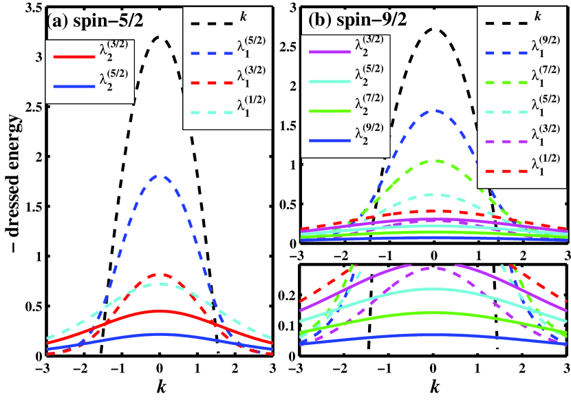
The dressed energy of charge rapidities $k$ in the ground state satisfies the following equations,

$\displaystyle\epsilon(k)=k^{2}-\mu+\hat{D}^{(s+1)}*\epsilon(k),~{}~{}|k|<Q,$
$\displaystyle\epsilon^{(l)}_{i}(k)=\hat{D}^{(l)}_{i}*\epsilon(k),\quad l=\frac{1}{2},\cdots,s.$ (28)

Here $\mu$ is the chemical potential, $*$ is an integral operation defined by $\hat{w}*y(x)=\int w(x-x^{\prime})y(x){\rm d}x^{\prime}$, $Q$ is the Fermi point which is determined by the particle density $n=N/L$, and the kernels $D(k)$ of integral operators $\hat{{D}}$ are

D​(k)=a^1/2βˆ—D1(s)​(k)+a^1βˆ—D2(s)​(k),D1(l)​(k)=12​s+1​sin⁑(2​lβˆ’12​s+1​π)cosh⁑(2​π​k/c2​s+1)+cos⁑(2​lβˆ’12​s+1​π),D2(l)​(k)=D^1(sβˆ’l+3/2)βˆ—D1(1/2)​(k),3/2≀l≀s,D(1/2)​(k)=1/[(2​s+3)​cosh⁑[π​k/(c​(s+3/2))]],formulae-sequenceformulae-sequenceπ·π‘˜subscript^π‘Ž12subscriptsuperscript𝐷𝑠1π‘˜subscript^π‘Ž1subscriptsuperscript𝐷𝑠2π‘˜formulae-sequencesubscriptsuperscript𝐷𝑙1π‘˜12𝑠12𝑙12𝑠1πœ‹2πœ‹π‘˜π‘2𝑠12𝑙12𝑠1πœ‹formulae-sequencesubscriptsuperscript𝐷𝑙2π‘˜subscriptsuperscript^𝐷𝑠𝑙321superscriptsubscript𝐷112π‘˜32𝑙𝑠superscript𝐷12π‘˜1delimited-[]2𝑠3πœ‹π‘˜π‘π‘ 32\begin{split}&{D}(k)=\hat{{a}}_{1/2}*{D}^{(s)}_{1}(k)+\hat{a}_{1}*{{D}}^{(s)}_{2}(k),\\ &{{D}}^{(l)}_{1}(k)=\frac{1}{2s+1}\frac{\sin(\frac{2l-1}{2s+1}\pi)}{\cosh(\frac{2\pi k/c}{2s+1})+\cos(\frac{2l-1}{2s+1}\pi)},\\ &{{D}}^{(l)}_{2}(k)=\hat{{D}}^{(s-l+3/2)}_{1}*{D}_{1}^{(1/2)}(k),~{}{3}/2\leq l\leq s,\\ &{{D}}^{(1/2)}(k)={1}/[(2s+3)\cosh[{\pi k}/{(c(s+3/2))}]],\end{split} (29)

where $a(x)=t/[\pi(x^{2}+(tc)^{2})]$. The dressed energy for $c=1$ and $n=1$ is shown in Fig. 2.

The physical properties of such 1D systems are controlled by the parameter $\gamma=c/n$ LiebLiniger1963PR . When $\gamma\to\infty$, we obtain the density of states, energy and Fermi point in the strong repulsive limit as

$$\rho(k)=\frac{1}{2\pi},(k\!\leq\!|Q|),~{}~{}E=\frac{1}{3\pi}Q^{3},~{}~{}Q=n\pi.$$ (30)

When $\gamma\to 0$, the system degenerates into the free fermions and we have

$$\rho(k)\!=\!\frac{2s\!+\!1}{2\pi},(k\!\leq\!|Q|),~{}E\!=\!\frac{2s\!+\!1}{3\pi}Q^{3},~{}Q\!=\!\frac{n\pi}{2s\!+\!1}.\!$$ (31)

VI Conclusion

In conclusion, we find that there is a hidden symmetry of the high spin cold atomic systems with a special interaction form away from the $SU(2s+1)$ symmetry point. Based on the symmetry analysis, a new class of integrable models for cold atoms with arbitrary spin is proposed.

VII Acknowledgments

We would like to thank Prof. Shu Chen, Xi-Wen Guan, Zhong-Qi Ma, M. T. Batchelor and G. V. Shlyapnikov for the beneficial discussions. This work was supported by the NSFC, the Knowledge Innovation Project of CAS, and the National Program for Basic Research of MOST.

* Email: yupeng@iphy.ac.cn

References

  • (1) Law C.Β K., Pu H. and Bigelow N.Β P., Phys. Rev. Lett., 81 (1998) 5257.
  • (2) Mukerjee S., Xu C. and Moore J.Β E., Phys. Rev. Lett., 97 (2006) 120406.
  • (3) Mueller E.Β J., Ho T.-L., Ueda M. and Baym G., Phys. Rev. A, 74 (2006) 033612.
  • (4) Bradley C.Β C., Sackett C.Β A., Tollett J.Β J. and Hulet R.Β G., Phys. Rev. Lett., 75 (1995) 1687;
    Bradley C.Β C., Sackett C.Β A. and Hulet R.Β G., Phys. Rev. Lett., 78 (1997) 985.
  • (5) Stamper-Kurn D.Β M., Andrews M.Β R., Chikkatur A.Β P., Inouye S., Miesner H.-J., Stenger J. and Ketterle W., Phys. Rev. Lett., 80 (1998) 2027;
    Stamper-Kurn D.Β M., Miesner H.-J., Chikkatur A.Β P., Inouye S., Stenger J. and Ketterle W., Phys. Rev. Lett., 81 (1998) 2194.
  • (6) Myatt C.Β J., Burt E.Β A., Ghrist R.Β W., Cornell E.Β A. and Wieman C.Β E., Phys. Rev. Lett., 78 (1997) 586.
  • (7) Barrett M.Β D., Sauer J.Β A. and Chapman M.Β S., Phys. Rev. Lett., 87 (2001) 010404.
  • (8) Paredes B., Widera A., Murg V., Mandel O., Folling S., Cirac I., Shlyapnikov G.Β V., Hansch T.Β W. and Bloch I., Nature, 429 (2004) 277.
  • (9) Chicireanu R., Pouderous A., BarbΓ© R., Laburthe-Tolra B., MarΓ©chal E., Vernac L., Keller J.-C. and Gorceix O., Phys. Rev. A, 73 (2006) 053406.
  • (10) DeMarco B. and Jin D.Β S., Science, 285 (1999) 1703.
  • (11) Takasu Y., Fukuhara T., Kitagawa M., Kumakura M. and Takahashi Y., Laser Phys., 16 (2006) 713.
  • (12) Witte A., Kisters T., Riehle F. and Helmcke J., J. Opt. Soc. Am. B, 9 (1992) 1030.
  • (13) Xu X., Loftus T.Β H., Hall J.Β L., Gallagher A. and Ye J., J. Opt. Soc. Am. B, 20 (2003) 968.
  • (14) SΓΆding J., GuΓ©ry-Odelin D., Desbiolles P., Ferrari G. and Dalibard J., Phys. Rev. Lett., 80 (1998) 1869.
  • (15) Ma Z.-Y., Foot C.Β J. and Cornish S.Β L., J. Phys. B: At. Mol. Opt. Phys., 37 (2004) 3187.
  • (16) Inouye S., Andrews M.Β R., Stenger J., Miesner H.-J., Stamper-Kurn D.Β M. and Ketterle W., Nature, 392 (1998) 151.
  • (17) Dickerscheid D. B.Β M., AlΒ Khawaja U., van Oosten D. and Stoof H. T.Β C., Phys. Rev. A, 71 (2005) 043604.
  • (18) Bergeman T., Moore M.Β G. and Olshanii M., Phys. Rev. Lett., 91 (2003) 163201.
  • (19) Ho T.-L., Phys. Rev. Lett., 81 (1998) 742.
  • (20) Ohmi T. and Machida K., J. Phys. Soc. Jpn., 67 (1998) 1822.
  • (21) Wu C., Phys. Rev. Lett., 95 (2005) 266404.
  • (22) Chen S., Wu C., Zhang S.-C. and Wang Y., Phys. Rev. B, 72 (2005) 214428.
  • (23) WU C., Mod. Phys. Lett. B, 20 (2006) 1707.
  • (24) Wu C., Hu J.-p. and Zhang S.-c., Phys. Rev. Lett., 91 (2003) 186402.
  • (25) Lieb E.Β H. and Liniger W., Phys. Rev., 130 (1963) 1605;
    Lieb E.Β H., Phys. Rev., 130 (1963) 1616.
  • (26) Yang C.Β N., Phys. Rev. Lett., 19 (1967) 1312;
    Yang C.Β N., Phys. Rev., 168 (1968) 1920.
  • (27) Sutherland B., Phys. Rev. Lett., 20 (1968) 98.
  • (28) Zhou Y.Β K., J. Phys. A: Math. Gen., 21 (1988) 2391;
    Zhou Y.Β K., J. Phys. A: Math. Gen., 21 (1988) 2399.
  • (29) Lai C.Β K. and Yang C.Β N., Phys. Rev. A, 3 (1971) 393;
    Lai C.Β K., J. Math. Phys., 15 (1974) 954.
  • (30) Pu F.-C., Wu Y.-Z. and Zhao B.-H., J. Phys. A: Math. Gen., 20 (1987) 1173;
    Fan H., Pu F.-C. and Zhao B.-H., J. Phys. A: Math. Gen., 22 (1989) 4835.
  • (31) Cao J., Jiang Y. and Wang Y., Europhys. Lett., 79 (2007) 30005.
  • (32) Jiang Y., Cao J. and Wang Y., Europhys. Lett., 87 (2009) 10006.
  • (33) Kulish P.Β P. and Sklyanin E.Β K., J. Sov. Math., 19 (1982) 1596.
  • (34) Kennedy T., J. Phys. A: Math. Gen., 25 (1992) 2809;
    Batchelor M.Β T. and Yung C.Β M., J. Phys. A: Math. Gen., 27 (1994) 5033.
  • (35) Martins M.Β J., Nucl. Phys. B, 636 (2002) 583.
  • (36) Martins M.Β J. and Ramos P.Β B., Nucl. Phys. B, 500 (1997) 579.