Erlangen Program at Large: Outline

Abstract.

This is an outline of Erlangen Program at Large. Study of objects and properties, which are invariant under a group action, is very fruitful far beyond the traditional geometry. In this paper we demonstrate this on the example of the group $SL_{2}{}(\mathbb{R}{})$. Starting from the conformal geometry we develop analytic functions and apply these to functional calculus. Finally we provide an extensive description of open problems.

1. Introduction

The simplest objects with non-commutative multiplication may be $2\times 2$ matrices with real entries. Such matrices of determinant one form a closed set under multiplication (since $\det(AB)=\det A\cdot\det B$), the identity matrix is among them and any such matrix has an inverse (since $\det A\neq 0$). In other words those matrices form a group, the $SL_{2}{}(\mathbb{R}{})$ group [Lang85]—one of the two most important Lie groups in analysis. The other group is the Heisenberg group [Howe80a]. By contrast the “$ax+b$”-group, which is often used to build wavelets, is only a subgroup of $SL_{2}{}(\mathbb{R}{})$, see the numerator in (1.1).

The simplest non-linear transforms of the real line—linear-fractional or Möbius maps—may also be associated with $2\times 2$ matrices [Beardon05a]*Ch. 13:

(1.1) $$g:x\mapsto g\cdot x=\frac{ax+b}{cx+d},\text{ where }g=\begin{pmatrix}a&b\\ c&d\end{pmatrix},x\in\mathbb{R}{}.$$

An enjoyable calculation shows that the composition of two transforms (1.1) with different matrices $g_{1}$ and $g_{2}$ is again a Möbius transform with matrix the product $g_{1}g_{2}$. In other words (1.1) it is a (left) action of $SL_{2}{}(\mathbb{R}{})$.

According to F. Klein’s Erlangen program (which was influenced by S. Lie) any geometry is dealing with invariant properties under a certain group action. For example, we may ask: What kinds of geometry are related to the $SL_{2}{}(\mathbb{R}{})$ action (1.1)?

The Erlangen program has probably the highest rate of $\frac{\text{praised}}{\text{actually used}}$ among mathematical theories not only due to the big numerator but also due to undeserving small denominator. As we shall see below Klein’s approach provides some surprising conclusions even for such over-studied objects as circles.

1.1. Make a Guess in Three Attempts

It is easy to see that the $SL_{2}{}(\mathbb{R}{})$ action (1.1) makes sense also as a map of complex numbers $z=x+\mathrm{i}y$, $\mathrm{i}^{2}=-1$. Moreover, if $y>0$ then $g\cdot z$ has a positive imaginary part as well, i.e. (1.1) defines a map from the upper half-plane to itself.

However there is no need to be restricted to the traditional route of complex numbers only. Less-known dual and double numbers [Yaglom79]*Suppl. C have also the form $z=x+\mathrm{i}y$ but different assumptions on the imaginary unit $\mathrm{i}$: $\mathrm{i}^{2}=0$ or $\mathrm{i}^{2}=1$ correspondingly. Although the arithmetic of dual and double numbers is different from the complex ones, e.g. they have divisors of zero, we are still able to define their transforms by (1.1) in most cases.

Three possible values $-1$, $0$ and $1$ of $\sigma:=\mathrm{i}^{2}$ will be refereed to here as elliptic, parabolic and hyperbolic cases respectively. We repeatedly meet such a division of various mathematical objects into three classes. They are named by the historically first example—the classification of conic sections—however the pattern persistently reproduces itself in many different areas: equations, quadratic forms, metrics, manifolds, operators, etc. We will abbreviate this separation as EPH-classification. The common origin of this fundamental division can be seen from the simple picture of a coordinate line split by zero into negative and positive half-axes:

(1.2)

Connections between different objects admitting EPH-classification are not limited to this common source. There are many deep results linking, for example, ellipticity of quadratic forms, metrics and operators. On the other hand there are still a lot of white spots and obscure gaps between some subjects as well.

To understand the action (1.1) in all EPH cases we use the Iwasawa decomposition [Lang85] of $SL_{2}{}(\mathbb{R}{})=ANK$ into three one-dimensional subgroups $A$, $N$ and $K$:

(1.3) $$\begin{pmatrix}a&b\\ c&d\end{pmatrix}={\begin{pmatrix}\alpha&0\\ 0&\alpha^{-1}\end{pmatrix}}{\begin{pmatrix}1&\nu\\ 0&1\end{pmatrix}}{\begin{pmatrix}\cos\phi&\sin\phi\\ -\sin\phi&\cos\phi\end{pmatrix}}.$$

Subgroups $A$ and $N$ act in (1.1) irrespectively to value of $\sigma$: $A$ makes a dilation by $\alpha^{2}$, i.e. $z\mapsto\alpha^{2}z$, and $N$ shifts points to left by $\nu$, i.e. $z\mapsto z+\nu$.

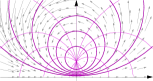
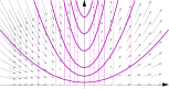
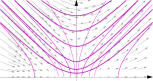
Figure 1. Action of the $K$ subgroup. The corresponding $K$-orbits are thick circles, parabolas and hyperbolas. Thin traversal lines are images of the vertical axis for certain values of the parameter $\phi$.

By contrast, the action of the third matrix from the subgroup $K$ sharply depends on $\sigma$, see Fig. 1. In elliptic, parabolic and hyperbolic cases $K$-orbits are circles, parabolas and (equilateral) hyperbolas correspondingly. Thin traversal lines in Fig. 1 join points of orbits for the same values of $\phi$ and grey arrows represent “local velocities”—vector fields of derived representations.

1.2. Erlangen program at large

As we already mentioned the division of mathematics into areas is only apparent. Therefore it is unnatural to limit Erlangen program only to “geometry”. We may continue to look for $SL_{2}{}(\mathbb{R}{})$ invariant objects in other related fields. For example, transform (1.1) generates unitary representations on certain $L_{2}{}$ spaces, cf. (1.1):

(1.4) $$g^{-1}:f(x)\mapsto\frac{1}{(cx+d)^{m}}f\left(\frac{ax+b}{cx+d}\right).$$

For $m=1$, $2$, …the invariant subspaces of $L_{2}{}$ are Hardy and (weighted) Bergman spaces of complex analytic functions. All main objects of complex analysis (Cauchy and Bergman integrals, Cauchy-Riemann and Laplace equations, Taylor series etc.) may be obtaining in terms of invariants of the discrete series representations of $SL_{2}{}(\mathbb{R}{})$ [Kisil02c]*§ 3. Moreover two other series (principal and complimentary [Lang85]) play the similar rôles for hyperbolic and parabolic cases [Kisil02c] [Kisil05a].

Moving further we may observe that transform (1.1) is defined also for an element $x$ in any algebra $\mathfrak{A}$ with a unit $\mathbf{1}$ as soon as $(cx+d\mathbf{1})\in\mathfrak{A}$ has an inverse. If $\mathfrak{A}$ is equipped with a topology, e.g. is a Banach algebra, then we may study a functional calculus for element $x$ [Kisil02a] in this way. It is defined as an intertwining operator between the representation (1.4) in a space of analytic functions and a similar representation in a left $\mathfrak{A}$-module.

In the spirit of Erlangen program such functional calculus is still a geometry, since it is dealing with invariant properties under a group action. However even for a simplest non-normal operator, e.g. a Jordan block of the length $k$, the obtained space is not like a space of point but is rather a space of $k$-th jets [Kisil02a]. Such non-point behaviour is oftenly attributed to non-commutative geometry and Erlangen program provides an important input on this fashionable topic [Kisil02c].

Of course, there is no reasons to limit Erlangen program to $SL_{2}{}(\mathbb{R}{})$ group only, other groups may be more suitable in different situations. However $SL_{2}{}(\mathbb{R}{})$ still possesses a big unexplored potential and is a good object to start with.

2. Geometry

2.1. Cycles as Invariant Objects

Definition 2.1.

The common name cycle [Yaglom79] is used to denote circles, parabolas and hyperbolas (as well as straight lines as their limits) in the respective EPH case.

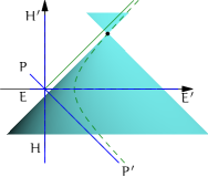
(a)                  (b)

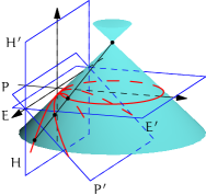
Figure 2. $K$-orbits as conic sections: circles are sections by the plane $EE^{\prime}$; parabolas are sections by $PP^{\prime}$; hyperbolas are sections by $HH^{\prime}$. Points on the same generator of the cone correspond to the same value of $\phi$.

It is well known that any cycle is a conic sections and an interesting observation is that corresponding $K$-orbits are in fact sections of the same two-sided right-angle cone, see Fig. 2. Moreover, each straight line generating the cone, see Fig. 2(b), is crossing corresponding EPH $K$-orbits at points with the same value of parameter $\phi$ from (1.3). In other words, all three types of orbits are generated by the rotations of this generator along the cone.

$K$-orbits are $K$-invariant in a trivial way. Moreover since actions of both $A$ and $N$ for any $\sigma$ are extremely “shape-preserving” we find natural invariant objects of the Möbius map:

Theorem 2.2 ([Kisil06a]).

The family of all cycles from Defn. 2.1 is invariant under the action (1.1).

According to Erlangen ideology we shall study invariant properties of cycles.

2.2. Invariance of FSCc

Fig. 2 suggests that we may get a unified treatment of cycles in all EPH by consideration of a higher dimension spaces. The standard mathematical method is to declare objects under investigations (cycles in our case, functions in functional analysis, etc.) to be simply points of some bigger space. This space should be equipped with an appropriate structure to hold externally information which were previously inner properties of our objects.

A generic cycle is the set of points $(u,v)\in\mathbb{R}^{2}{}$ defined for all values of $\sigma$ by the equation

(2.1) $$k(u^{2}-\sigma v^{2})-2lu-2nv+m=0.$$

This equation (and the corresponding cycle) is defined by a point $(k,l,n,m)$ from a projective space $\mathbb{P}^{3}{}$, since for a scaling factor $\lambda\neq 0$ the point $(\lambda k,\lambda l,\lambda n,\lambda m)$ defines the same equation (2.1). We call $\mathbb{P}^{3}{}$ the cycle space and refer to the initial $\mathbb{R}^{2}{}$ as the point space.

In order to get a connection with Möbius action (1.1) we arrange numbers $(k,l,n,m)$ into the matrix

(2.2) $$C_{\breve{\sigma}}^{s}=\begin{pmatrix}l+\mathrm{\breve{\i}}sn&-m\\ k&-l+\mathrm{\breve{\i}}sn\end{pmatrix},$$

with a new imaginary unit $\mathrm{\breve{\i}}$ and an additional parameter $s$ usually equal to $\pm 1$. The values of $\breve{\sigma}:=\mathrm{\breve{\i}}^{2}$ is $-1$, $0$ or $1$ independently from the value of $\sigma$. The matrix (2.2) is the cornerstone of (extended) Fillmore–Springer–Cnops construction (FSCc) [Cnops02a] and closely related to technique recently used by A.A. Kirillov to study the Apollonian gasket [Kirillov06].

The significance of FSCc in Erlangen framework is provided by the following result:

Theorem 2.3.

The image $\tilde{C}_{\breve{\sigma}}^{s}$ of a cycle $C_{\breve{\sigma}}^{s}$ under transformation (1.1) with $g\in SL_{2}{}(\mathbb{R}{})$ is given by similarity of the matrix (2.2):

(2.3) $$\tilde{C}_{\breve{\sigma}}^{s}=gC_{\breve{\sigma}}^{s}g^{-1}.$$

In other words FSCc (2.2) intertwines Möbius action (1.1) on cycles with linear map (2.3).

There are several ways to prove (2.3): either by a brute force calculation (fortunately performed by a CAS) [Kisil05a] or through the related orthogonality of cycles [Cnops02a], see the end of the next section 2.3.

The important observation here is that FSCc (2.2) uses an imaginary unit $\mathrm{\breve{\i}}$ which is not related to $\mathrm{i}$ defining the appearance of cycles on plane. In other words any EPH type of geometry in the cycle space $\mathbb{P}^{3}{}$ admits drawing of cycles in the point space $\mathbb{R}^{2}{}$ as circles, parabolas or hyperbolas. We may think on points of $\mathbb{P}^{3}{}$ as ideal cycles while their depictions on $\mathbb{R}^{2}{}$ are only their shadows on the wall of Plato’s cave.

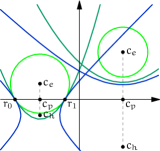
(a)           (b)

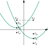
Figure 3. (a) Different EPH implementations of the same cycles defined by quadruples of numbers.
(b) Centres and foci of two parabolas with the same focal length.

Fig. 3(a) shows the same cycles drawn in different EPH styles. Points $c_{e,p,h}=(\frac{l}{k},-\sigma\frac{n}{k})$ are their respective e/p/h-centres. They are related to each other through several identities:

(2.4) $$c_{e}=\bar{c}_{h},\quad c_{p}=\frac{1}{2}(c_{e}+c_{h}).$$

Fig. 3(b) presents two cycles drawn as parabolas, they have the same focal length $\frac{n}{2k}$ and thus their e-centres are on the same level. In other words concentric parabolas are obtained by a vertical shift, not scaling as an analogy with circles or hyperbolas may suggest.

Fig. 3(b) also presents points, called e/p/h-foci:

(2.5) $$f_{e,p,h}=\left(\frac{l}{k},-\frac{\det C_{\breve{\sigma}}^{s}}{2nk}\right),$$

which are independent of the sign of $s$. If a cycle is depicted as a parabola then h-focus, p-focus, e-focus are correspondingly geometrical focus of the parabola, its vertex, and the point on the directrix nearest to the vertex.

As we will see, cf. Thms. 2.5 and 2.7, all three centres and three foci are useful attributes of a cycle even if it is drawn as a circle.

2.3. Invariants: algebraic and geometric

We use known algebraic invariants of matrices to build appropriate geometric invariants of cycles. It is yet another demonstration that any division of mathematics into subjects is only illusive.

For $2\times 2$ matrices (and thus cycles) there are only two essentially different invariants under similarity (2.3) (and thus under Möbius action (1.1)): the trace and the determinant. The latter was already used in (2.5) to define cycle’s foci. However due to projective nature of the cycle space $\mathbb{P}^{3}{}$ the absolute values of trace or determinant are irrelevant, unless they are zero.

Alternatively we may have a special arrangement for normalisation of quadruples $(k,l,n,m)$. For example, if $k\neq 0$ we may normalise the quadruple to $(1,\frac{l}{k},\frac{n}{k},\frac{m}{k})$ with highlighted cycle’s centre. Moreover in this case $\det{C^{s}_{\breve{\sigma}}}$ is equal to the square of cycle’s radius, cf. Section 2.6. Another normalisation $\det{C^{s}_{\breve{\sigma}}}=1$ is used in [Kirillov06] to get a nice condition for touching circles.

We still get important characterisation even with non-normalised cycles, e.g., invariant classes (for different $\breve{\sigma}$) of cycles are defined by the condition $\det C_{\breve{\sigma}}^{s}=0$. Such a class is parametrises only by two real number and as such is easily attached to certain point of $\mathbb{R}^{2}{}$. For example, the cycle $C_{\breve{\sigma}}^{s}$ with $\det C_{\breve{\sigma}}^{s}=0$, $\breve{\sigma}=-1$ drawn elliptically represent just a point $(\frac{l}{k},\frac{n}{k})$, i.e. (elliptic) zero-radius circle. The same condition with $\breve{\sigma}=1$ in hyperbolic drawing produces a null-cone originated at point $(\frac{l}{k},\frac{n}{k})$:

$$(u-\frac{l}{k})^{2}-(v-\frac{n}{k})^{2}=0,$$

i.e. a zero-radius cycle in hyperbolic metric.

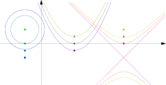
Figure 4. Different $\mathrm{i}$-implementations of the same $\breve{\sigma}$-zero-radius cycles and corresponding foci.

In general for every notion there is nine possibilities: three EPH cases in the cycle space times three EPH realisations in the point space. Such nine cases for “zero radius” cycles is shown on Fig. 4. For example, p-zero-radius cycles in any implementation touch the real axis.

This “touching” property is a manifestation of the boundary effect in the upper-half plane geometry [Kisil05a]*Rem. 3.4. The famous question on hearing drum’s shape has a sister:

Can we see/feel the boundary from inside a domain?

Both orthogonality relations described below are “boundary aware” as well. It is not surprising after all since $SL_{2}{}(\mathbb{R}{})$ action on the upper-half plane was obtained as an extension of its action (1.1) on the boundary.

According to the categorical viewpoint internal properties of objects are of minor importance in comparison to their relations with other objects from the same class. Thus from now on we will look for invariant relations between two or more cycles.

2.4. Joint invariants: orthogonality

The most expected relation between cycles is based on the following Möbius invariant “inner product” build from a trace of product of two cycles as matrices:

(2.6) $$\left\langle C_{\breve{\sigma}}^{s},\tilde{C}_{\breve{\sigma}}^{s}\right\rangle=\mathop{tr}(C_{\breve{\sigma}}^{s}\tilde{C}_{\breve{\sigma}}^{s})$$

By the way, an inner product of this type is used, for example, in GNS construction to make a Hilbert space out of $C^{*}$-algebra. The next standard move is given by the following definition.

Definition 2.4.

Two cycles are called $\breve{\sigma}$-orthogonal if $\left\langle C_{\breve{\sigma}}^{s},\tilde{C}_{\breve{\sigma}}^{s}\right\rangle=0$.

For the case of $\breve{\sigma}\sigma=1$, i.e. when geometries of the cycle and point spaces are both either elliptic or hyperbolic, such an orthogonality is the standard one, defined in terms of angles between tangent lines in the intersection points of two cycles. However in the remaining seven ($=9-2$) cases the innocent-looking Defn. 2.4 brings unexpected relations.

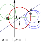
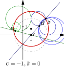
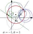
Figure 5. Orthogonality of the first kind in the elliptic point space.
Each picture presents two groups (green and blue) of cycles which are orthogonal to the red cycle $C^{s}_{\breve{\sigma}}$. Point $b$ belongs to $C^{s}_{\breve{\sigma}}$ and the family of blue cycles passing through $b$ is orthogonal to $C^{s}_{\breve{\sigma}}$. They all also intersect in the point $d$ which is the inverse of $b$ in $C^{s}_{\breve{\sigma}}$. Any orthogonality is reduced to the usual orthogonality with a new (“ghost”) cycle (shown by the dashed line), which may or may not coincide with $C^{s}_{\breve{\sigma}}$. For any point $a$ on the “ghost” cycle the orthogonality is reduced to the local notion in the terms of tangent lines at the intersection point. Consequently such a point $a$ is always the inverse of itself.

Elliptic (in the point space) realisations of Defn. 2.4, i.e. $\sigma=-1$ is shown in Fig. 5. The left picture corresponds to the elliptic cycle space, e.g. $\breve{\sigma}=-1$. The orthogonality between the red circle and any circle from the blue or green families is given in the usual Euclidean sense. The central (parabolic in the cycle space) and the right (hyperbolic) pictures show non-local nature of the orthogonality. There are analogues pictures in parabolic and hyperbolic point spaces as well [Kisil05a].

This orthogonality may still be expressed in the traditional sense if we will associate to the red circle the corresponding “ghost” circle, which shown by the dashed line in Fig. 5. To describe ghost cycle we need the Heaviside function $\chi(\sigma)$:

(2.7) $$\chi(t)=\left\{\begin{array}[]{ll}1,&t\geq 0;\\ -1,&t<0.\end{array}\right.$$

Theorem 2.5.

A cycle is $\breve{\sigma}$-orthogonal to cycle $C_{\breve{\sigma}}^{s}$ if it is orthogonal in the usual sense to the $\sigma$-realisation of “ghost” cycle $\hat{C}_{\breve{\sigma}}^{s}$, which is defined by the following two conditions:

1. $\chi(\sigma)$-centre of $\hat{C}_{\breve{\sigma}}^{s}$ coincides with $\breve{\sigma}$-centre of $C_{\breve{\sigma}}^{s}$.

2. Cycles $\hat{C}_{\breve{\sigma}}^{s}$ and $C^{s}_{\breve{\sigma}}$ have the same roots, moreover $\det\hat{C}_{\sigma}^{1}=\det C^{\chi(\breve{\sigma})}_{\sigma}$.

The above connection between various centres of cycles illustrates their meaningfulness within our approach.

One can easy check the following orthogonality properties of the zero-radius cycles defined in the previous section:

1. Since $\left\langle C_{\breve{\sigma}}^{s},{C}_{\breve{\sigma}}^{s}\right\rangle=\det{C}_{\breve{\sigma}}^{s}$ zero-radius cycles are self-orthogonal (isotropic) ones.

2. A cycle ${C^{s}_{\breve{\sigma}}}$ is $\sigma$-orthogonal to a zero-radius cycle $Z^{s}_{\breve{\sigma}}$ if and only if ${C^{s}_{\breve{\sigma}}}$ passes through the $\sigma$-centre of $Z^{s}_{\breve{\sigma}}$.

2.5. Higher order joint invariants: s-orthogonality

With appetite already wet one may wish to build more joint invariants. Indeed for any homogeneous polynomial $p(x_{1},x_{2},\ldots,x_{n})$ of several non-commuting variables one may define an invariant joint disposition of $n$ cycles ${}^{j}\!{C^{s}_{\breve{\sigma}}}$ by the condition:

$$\mathop{tr}p({}^{1}\!{C^{s}_{\breve{\sigma}}},{}^{2}\!{C^{s}_{\breve{\sigma}}},\ldots,{}^{n}\!{C^{s}_{\breve{\sigma}}})=0.$$

However it is preferable to keep some geometrical meaning of constructed notions.

An interesting observation is that in the matrix similarity of cycles (2.3) one may replace element $g\in SL_{2}{}(\mathbb{R}{})$ by an arbitrary matrix corresponding to another cycle. More precisely the product ${C^{s}_{\breve{\sigma}}}{\tilde{C}^{s}_{\breve{\sigma}}}{C^{s}_{\breve{\sigma}}}$ is again the matrix of the form (2.2) and thus may be associated to a cycle. This cycle may be considered as the reflection of ${\tilde{C}^{s}_{\breve{\sigma}}}$ in ${C^{s}_{\breve{\sigma}}}$.

Definition 2.6.

A cycle ${C^{s}_{\breve{\sigma}}}$ is s-orthogonal to a cycle ${\tilde{C}^{s}_{\breve{\sigma}}}$ if the reflection of ${\tilde{C}^{s}_{\breve{\sigma}}}$ in ${C^{s}_{\breve{\sigma}}}$ is orthogonal (in the sense of Defn. 2.4) to the real line. Analytically this is defined by:

(2.8) $$\mathop{tr}({C^{s}_{\breve{\sigma}}}{\tilde{C}^{s}_{\breve{\sigma}}}{C^{s}_{\breve{\sigma}}}R^{s}_{\breve{\sigma}})=0.$$

Due to invariance of all components in the above definition s-orthogonality is a Möbius invariant condition. Clearly this is not a symmetric relation: if ${C^{s}_{\breve{\sigma}}}$ is s-orthogonal to ${\tilde{C}^{s}_{\breve{\sigma}}}$ then ${\tilde{C}^{s}_{\breve{\sigma}}}$ is not necessarily s-orthogonal to ${C^{s}_{\breve{\sigma}}}$.

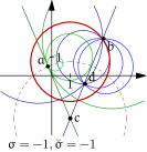
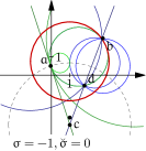
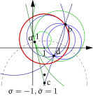
Figure 6. Orthogonality of the second kind for circles. To highlight both similarities and distinctions with the ordinary orthogonality we use the same notations as that in Fig. 5.

Fig. 6 illustrates s-orthogonality in the elliptic point space. By contrast with Fig. 5 it is not a local notion at the intersection points of cycles for all $\breve{\sigma}$. However it may be again clarified in terms of the appropriate s-ghost cycle, cf. Thm. 2.5.

Theorem 2.7.

A cycle is s-orthogonal to a cycle $C^{s}_{\breve{\sigma}}$ if its orthogonal in the traditional sense to its s-ghost cycle ${\tilde{C}^{\breve{\sigma}}_{\breve{\sigma}}}={C^{\chi(\sigma)}_{\breve{\sigma}}}\mathbb{R}^{\breve{\sigma}}_{\breve{\sigma}}{}{C^{\chi(\sigma)}_{\breve{\sigma}}}$, which is the reflection of the real line in ${C^{\chi(\sigma)}_{\breve{\sigma}}}$ and $\chi$ is the Heaviside function (2.7). Moreover

1. $\chi(\sigma)$-Centre of ${\tilde{C}^{\breve{\sigma}}_{\breve{\sigma}}}$ coincides with the $\breve{\sigma}$-focus of ${C^{s}_{\breve{\sigma}}}$, consequently all lines s-orthogonal to ${C^{s}_{\breve{\sigma}}}$ are passing the respective focus.

2. Cycles ${C^{s}_{\breve{\sigma}}}$ and ${\tilde{C}^{\breve{\sigma}}_{\breve{\sigma}}}$ have the same roots.

Note the above intriguing interplay between cycle’s centres and foci. Although s-orthogonality may look exotic it will naturally appear in the end of next Section again.

Of course, it is possible to define another interesting higher order joint invariants of two or even more cycles.

2.6. Distance, length and perpendicularity

Geometry in the plain meaning of this word deals with distances and lengths. Can we obtain them from cycles?

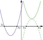
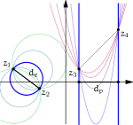
(a) (b) (c)

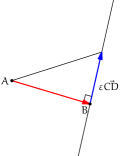
Figure 7. (a) The square of the parabolic diameter is the square of the distance between roots if they are real ($z_{1}$ and $z_{2}$), otherwise the negative square of the distance between the adjoint roots ($z_{3}$ and $z_{4}$).
(b) Distance as extremum of diameters in elliptic ($z_{1}$ and $z_{2}$) and parabolic ($z_{3}$ and $z_{4}$) cases.
(c) Perpendicular as the shortest route to a line.

We mentioned already that for circles normalised by the condition $k=1$ the value $\det{C^{s}_{\breve{\sigma}}}=\left\langle{C^{s}_{\breve{\sigma}}},{C^{s}_{\breve{\sigma}}}\right\rangle$ produces the square of the traditional circle radius. Thus we may keep it as the definition of the radius for any cycle. But then we need to accept that in the parabolic case the radius is the (Euclidean) distance between (real) roots of the parabola, see Fig. 7(a).

Having radii of circles already defined we may use them for other measurements in several different ways. For example, the following variational definition may be used:

Definition 2.8.

The distance between two points is the extremum of diameters of all cycles passing through both points, see Fig. 7(b).

If $\breve{\sigma}=\sigma$ this definition gives in all EPH cases the distance between endpoints of a vector $z=u+\mathrm{i}v$ as follows:

(2.9) $$d_{e,p,h}(u,v)^{2}=(u+\mathrm{i}v)(u-\mathrm{i}v)=u^{2}-\sigma v^{2}.$$

The parabolic distance $d_{p}^{2}=u^{2}$, see Fig. 7(b), algebraically sits between $d_{e}$ and $d_{h}$ according to the general principle (1.2) and is widely accepted [Yaglom79]. However one may be unsatisfied by its degeneracy.

An alternative measurement is motivated by the fact that a circle is the set of equidistant points from its centre. However the choice of “centre” is now rich: it may be either point from three centres (2.4) or three foci (2.5).

Definition 2.9.

The length of a directed interval $\overrightarrow{AB}$ is the radius of the cycle with its centre (denoted by $l_{c}(\overrightarrow{AB})$) or focus (denoted by $l_{f}(\overrightarrow{AB})$) at the point $A$ which passes through $B$.

These definition is less common and have some unusual properties like non-symmetry: $l_{f}(\overrightarrow{AB})\neq l_{f}(\overrightarrow{BA})$. However it comfortably fits the Erlangen program due to its $SL_{2}{}(\mathbb{R}{})$-conformal invariance:

Theorem 2.10 ([Kisil05a]).

Let $l$ denote either the EPH distances (2.9) or any length from Defn. 2.9. Then for fixed $y$, $y^{\prime}\in\mathbb{R}^{\sigma}{}$ the limit:

$$\lim_{t\rightarrow 0}\frac{l(g\cdot y,g\cdot(y+ty^{\prime}))}{l(y,y+ty^{\prime})},\qquad\text{ where }g\in SL_{2}{}(\mathbb{R}{}),$$

exists and its value depends only from $y$ and $g$ and is independent from $y^{\prime}$.

We may return from distances to angles recalling that in the Euclidean space a perpendicular provides the shortest root from a point to a line, see Fig. 7(c).

Definition 2.11.

Let $l$ be a length or distance. We say that a vector $\overrightarrow{AB}$ is $l$-perpendicular to a vector $\overrightarrow{CD}$ if function $l(\overrightarrow{AB}+\varepsilon\overrightarrow{CD})$ of a variable $\varepsilon$ has a local extremum at $\varepsilon=0$.

A pleasant surprise is that $l_{f}$-perpendicularity obtained thought the length from focus (Defn. 2.9) coincides with already defined in Section 2.5 s-orthogonality as follows from Thm. 2.7(i). It is also possible [Kisil08a] to make $SL_{2}{}(\mathbb{R}{})$ action isometric in all three cases.

All these study are waiting to be generalised to high dimensions and Clifford algebras provide a suitable language for this [Kisil05a].

3. Analytic Functions

We saw in the previous section that an inspiring geometry of cycles can be recovered from the properties of $SL_{2}{}(\mathbb{R}{})$. In this section we consider a realisation of the function theory within Erlangen approach [Kisil97c, Kisil97a, Kisil01a, Kisil02c].

3.1. Wavelet Transform and Cauchy Kernel

Elements of $SL_{2}{}(\mathbb{R}{})$ could be also represented by $2\times 2$-matrices with complex entries such that:

$$g={\left(\!\!\begin{array}[]{cc}\alpha&\bar{\beta}\\ \beta&\bar{\alpha}\end{array}\!\!\right)},\qquad g^{-1}={\left(\!\!\begin{array}[]{cc}\bar{\alpha}&-\bar{\beta}\\ -\beta&\alpha\end{array}\!\!\right)},\qquad\left|\alpha\right|^{2}-\left|\beta\right|^{2}=1.$$

This realisations of $SL_{2}{}(\mathbb{R}{})$ (or rather $SU(2,\mathbb{C}{})$) is more suitable for function theory in the unit disk. It is obtained from the form, which we used before for the upper half-plane, by means of the Cayley transform [Kisil05a, § 8.1].

We may identify the unit disk $\mathbb{D}{}$ with the homogeneous space $SL_{2}{}(\mathbb{R}{})/\mathbb{T}{}$ for the unit circle $\mathbb{T}{}$ through the important decomposition $SL_{2}{}(\mathbb{R}{})\sim\mathbb{D}{}\times\mathbb{T}{}$ with $K=\mathbb{T}{}$—the only compact subgroup of $SL_{2}{}(\mathbb{R}{})$:

(3.7) $${\left(\!\!\begin{array}[]{cc}\alpha&\bar{\beta}\\ \beta&\bar{\alpha}\end{array}\!\!\right)} = \left|\alpha\right|{\left(\!\!\begin{array}[]{cc}1&\bar{\beta}\bar{\alpha}^{-1}\\ {\beta}{\alpha}^{-1}&1\end{array}\!\!\right)}{\left(\!\!\begin{array}[]{cc}\frac{{\alpha}}{\left|\alpha\right|}&0\\ 0&\frac{\bar{\alpha}}{\left|\alpha\right|}\end{array}\!\!\right)}$$

(3.12) $$= \frac{1}{\sqrt{1-\left|u\right|^{2}}}{\left(\!\!\begin{array}[]{cc}1&u\\ \bar{u}&1\end{array}\!\!\right)},{\left(\!\!\begin{array}[]{cc}e^{i\omega}&0\\ 0&e^{-i\omega}\end{array}\!\!\right)}$$

where

$$\omega=\arg\alpha,\qquad u=\bar{\beta}\bar{\alpha}^{-1},\qquad\left|u\right|<1.$$

Each element $g\in SL_{2}{}(\mathbb{R}{})$ acts by the linear-fractional transformation (the Möbius map) on $\mathbb{D}{}$ and $\mathbb{T}{}$ $H_{2}{}(\mathbb{T}{})$ as follows:

(3.13) $$g^{-1}:z\mapsto\frac{\bar{\alpha}z-\bar{\beta}}{\alpha-{\beta}z},\qquad\textrm{ where }\quad g^{-1}={\left(\!\!\begin{array}[]{cc}\bar{\alpha}&-\bar{\beta}\\ -\beta&\alpha\end{array}\!\!\right)}.$$

In the decomposition (3.7) the first matrix on the right hand side acts by transformation (1.1) as an orthogonal rotation of $\mathbb{T}{}$ or $\mathbb{D}{}$; and the second one—by transitive family of maps of the unit disk onto itself.

The standard linearisation procedure [Kirillov76, § 7.1] leads from Möbius transformations (1.1) to the unitary representation $\rho_{1}$ irreducible on the Hardy space:

(3.14) $$\rho_{1}(g):f(z)\mapsto\frac{1}{\alpha-{\beta}{z}}\,f\left(\frac{\bar{\alpha}z-\bar{\beta}}{\alpha-{\beta}z}\right)\qquad\textrm{ where }\quad g^{-1}={\left(\!\!\begin{array}[]{cc}\bar{\alpha}&-\bar{\beta}\\ -\beta&\alpha\end{array}\!\!\right)}.$$

Möbius transformations provide a natural family of intertwining operators for $\rho_{1}$ coming from inner automorphisms of $SL_{2}{}(\mathbb{R}{})$ (will be used later).

We choose [Kisil98a, Kisil01a] $K$-invariant function $v_{0}(z)\equiv 1$ to be a vacuum vector. Thus the associated coherent states

$$v(g,z)=\rho_{1}(g)v_{0}(z)=(u-z)^{-1}$$

are completely determined by the point on the unit disk $u=\bar{\beta}\bar{\alpha}^{-1}$. The family of coherent states considered as a function of both $u$ and $z$ is obviously the Cauchy kernel [Kisil97c]. The wavelet transform [Kisil97c, Kisil98a] $\mathcal{W}:L_{2}{}(\mathbb{T}{})\rightarrow H_{2}{}(\mathbb{D}{}):f(z)\mapsto\mathcal{W}f(g)=\left\langle f,v_{g}\right\rangle$ is the Cauchy integral:

(3.15) $$\mathcal{W}f(u)=\frac{1}{2\pi i}\int_{\mathbb{T}{}}f(z)\frac{1}{u-z}\,dz.$$

We start from the following observation reflected in the almost any textbook on complex analysis:

Proposition 3.1.

Analytic function theory in the unit disk $\mathbb{D}{}$ is a manifestation of the mock discrete series representation $\rho_{1}$ of $SL_{2}{}(\mathbb{R}{})$:

(3.16) $$\rho_{1}(g):f(z)\mapsto\frac{1}{\alpha-{\beta}{z}}\,f\left(\frac{\bar{\alpha}z-\bar{\beta}}{\alpha-{\beta}z}\right),\quad\textup{ where }{\left(\!\!\begin{array}[]{cc}\bar{\alpha}&-\bar{\beta}\\ -\beta&\alpha\end{array}\!\!\right)}\in SL_{2}{}(\mathbb{R}{}).$$

Other classical objects of complex analysis (the Cauchy-Riemann equation, the Taylor series, the Bergman space, etc.) can be also obtained [Kisil97c, Kisil01a] from representation $\rho_{1}$ as shown below.

3.2. The Dirac (Cauchy-Riemann) and Laplace Operators

Consideration of Lie groups is hardly possible without consideration of their Lie algebras, which are naturally represented by left and right invariant vectors fields on groups. On a homogeneous space $\Omega=G/H$ we have also defined a left action of $G$ and can be interested in left invariant vector fields (first order differential operators). Due to the irreducibility of $F_{2}{}(\Omega)$ under left action of $G$ every such vector field $D$ restricted to $F_{2}{}(\Omega)$ is a scalar multiplier of identity $D|_{F_{2}{}(\Omega)}=cI$. We are in particular interested in the case $c=0$.

Definition 3.2.

[AtiyahSchmid80, KnappWallach76] A $G$-invariant first order differential operator

$$D_{\tau}:C_{\infty}{}(\Omega,\mathcal{S}\otimes V_{\tau})\rightarrow C_{\infty}{}(\Omega,\mathcal{S}\otimes V_{\tau})$$

such that $\mathcal{W}(F_{2}{}(X))\subset\mathrm{ker}\,D_{\tau}$ is called (Cauchy-Riemann-)Dirac operator on $\Omega=G/H$ associated with an irreducible representation $\tau$ of $H$ in a space $V_{\tau}$ and a spinor bundle $\mathcal{S}$.

The Dirac operator is explicitly defined by the formula [KnappWallach76, (3.1)]:

(3.17) $$D_{\tau}=\sum_{j=1}^{n}\rho(Y_{j})\otimes c(Y_{j})\otimes 1,$$

where $Y_{j}$ is an orthonormal basis of $\mathfrak{p}=\mathfrak{h}^{\perp}$—the orthogonal completion of the Lie algebra $\mathfrak{h}$ of the subgroup $H$ in the Lie algebra $\mathfrak{g}$ of $G$; $\rho(Y_{j})$ is the infinitesimal generator of the right action of $G$ on $\Omega$; $c(Y_{j})$ is Clifford multiplication by $Y_{i}\in\mathfrak{p}$ on the Clifford module $\mathcal{S}$. We also define an invariant Laplacian by the formula

(3.18) $$\Delta_{\tau}=\sum_{j=1}^{n}\rho(Y_{j})^{2}\otimes\epsilon_{j}\otimes 1,$$

where $\epsilon_{j}=c(Y_{j})^{2}$ is $+1$ or $-1$.

Proposition 3.3.

Let all commutators of vectors of $\mathfrak{h}^{\perp}$ belong to $\mathfrak{h}$, i.e. $[\mathfrak{h}^{\perp},\mathfrak{h}^{\perp}]\subset\mathfrak{h}$. Let also $f_{0}$ be an eigenfunction for all vectors of $\mathfrak{h}$ with eigenvalue $0$ and let also $\mathcal{W}f_{0}$ be a null solution to the Dirac operator $D$. Then $\Delta f(x)=0$ for all $f(x)\in F_{2}{}(\Omega)$.

Proof.

Because $\Delta$ is a linear operator and $F_{2}{}(\Omega)$ is generated by $\pi_{0}(s(a))\mathcal{W}f_{0}$ it is enough to check that $\Delta\pi_{0}(s(a))\mathcal{W}f_{0}=0$. Because $\Delta$ and $\pi_{0}$ commute it is enough to check that $\Delta\mathcal{W}f_{0}=0$. Now we observe that

$$\Delta=D^{2}-\sum_{i,j}\rho([Y_{i},Y_{j}])\otimes c(Y_{i})c(Y_{j})\otimes 1.$$

Thus the desired assertion is follows from two identities $\rho([Y_{i},Y_{j}])\mathcal{W}f_{0}=0$ for $[Y_{i},Y_{j}]\in H$ and $D\mathcal{W}f_{0}=0$. ∎

Example 3.4.

Let $G=SL_{2}{}(\mathbb{R}{})$ and $H$ be its one-dimensional compact subgroup $K$ generated by an element $Z\in\mathfrak{sl}(2,\mathbb{R}{})$. Then $\mathfrak{h}^{\perp}$ is spanned by two vectors $Y_{1}=A$ and $Y_{2}=B$. In such a situation we can use $\mathbb{C}{}$ instead of the Clifford algebra. Then formula (3.17) takes a simple form $D=r(A+iB)$. Infinitesimal action of this operator in the upper-half plane follows from calculation in [Lang85, VI.5(8), IX.5(3)], it is $[D_{\mathbb{H}{}}f](z)=-2iy\frac{\partial f(z)}{\partial\bar{z}}$, $z=x+iy$. Making the Caley transform we can find its action in the unit disk $D_{\mathbb{D}{}}$: again the Cauchy-Riemann operator $\frac{\partial}{\partial\bar{z}}$ is its principal component. We calculate $D_{\mathbb{H}{}}$ explicitly now to stress the similarity with $\mathbb{R}^{1,1}{}$ case.

For the upper half plane $\mathbb{H}{}$ we have following formulas:

$$s : \mathbb{H}{}\rightarrow SL_{2}{}(\mathbb{R}{}):z=x+iy\mapsto g={\left(\!\!\begin{array}[]{cc}y^{1/2}&xy^{-1/2}\\ 0&y^{-1/2}\end{array}\!\!\right)};$$

$$s^{-1} : SL_{2}{}(\mathbb{R}{})\rightarrow\mathbb{H}{}:{\left(\!\!\begin{array}[]{cc}a&b\\ c&d\end{array}\!\!\right)}\mapsto z=\frac{ai+b}{ci+d};$$

$$\rho(g) : \mathbb{H}{}\rightarrow\mathbb{H}{}:z\mapsto s^{-1}(s(z)*g)$$

$$\qquad\qquad\qquad=s^{-1}{\left(\!\!\begin{array}[]{cc}ay^{-1/2}+cxy^{-1/2}&by^{1/2}+dxy^{-1/2}\\ cy^{-1/2}&dy^{-1/2}\end{array}\!\!\right)}$$

$$\qquad\qquad\qquad=\frac{(yb+xd)+i(ay+cx)}{ci+d}$$

Thus the right action of $SL_{2}{}(\mathbb{R}{})$ on $\mathbb{H}{}$ is given by the formula

$$\rho(g)z=\frac{(yb+xd)+i(ay+cx)}{ci+d}=x+y\frac{bd+ac}{c^{2}+d^{2}}+iy\frac{1}{c^{2}+d^{2}}.$$

For $A$ and $B$ in $\mathfrak{sl}(2,\mathbb{R}{})$ we have:

$$\rho(e^{At})z=x+iye^{2t},\qquad\rho(e^{Bt})z=x+y\frac{e^{2t}-e^{-2t}}{e^{2t}+e^{-2t}}+iy\frac{4}{e^{2t}+e^{-2t}}.$$

Thus

$$[\rho(A)f](z) = \frac{\partial f(\rho(e^{At})z)}{\partial t}|_{t=0}=2y\partial_{2}f(z),$$

$${}[\rho(B)f](z) = \frac{\partial f(\rho(e^{Bt})z)}{\partial t}|_{t=0}=2y\partial_{1}f(z),$$

where $\partial_{1}$ and $\partial_{2}$ are derivatives of $f(z)$ with respect to real and imaginary party of $z$ respectively. Thus we get

$$D_{\mathbb{H}{}}=i\rho(A)+\rho(B)=2yi\partial_{2}+2y\partial_{1}=2y\frac{\partial}{\partial\bar{z}}$$

as was expected.

3.3. The Taylor expansion

For any decomposition $f_{a}(x)=\sum_{\alpha}\psi_{\alpha}(x)V_{\alpha}(a)$ of the coherent states $f_{a}(x)$ by means of functions $V_{\alpha}(a)$ (where the sum can become eventually an integral) we have the Taylor expansion

(3.22) $$\widehat{f}(a) = \int_{X}f(x)\bar{f}_{a}(x)\,dx=\int_{X}f(x)\sum_{\alpha}\bar{\psi}_{\alpha}(x)\bar{V}_{\alpha}(a)\,dx$$

$$= \sum_{\alpha}\int_{X}f(x)\bar{\psi}_{\alpha}(x)\,dx\bar{V}_{\alpha}(a)$$

$$= \sum_{\alpha}^{\infty}\bar{V}_{\alpha}(a)f_{\alpha},$$

where $f_{\alpha}=\int_{X}f(x)\bar{\psi}_{\alpha}(x)\,dx$. However to be useful within the presented scheme such a decomposition should be connected with the structures of $G$, $H$, and the representation $\pi_{0}$. We will use a decomposition of $f_{a}(x)$ by the eigenfunctions of the operators $\pi_{0}(h)$, $h\in\mathfrak{h}$.

Definition 3.5.

Let $F_{2}{}=\int_{A}H_{\alpha}{}\,d\alpha$ be a spectral decomposition with respect to the operators $\pi_{0}(h)$, $h\in\mathfrak{h}$. Then the decomposition

(3.23) $$f_{a}(x)=\int_{A}V_{\alpha}(a)f_{\alpha}(x)\,d\alpha,$$

where $f_{\alpha}(x)\in H_{\alpha}{}$ and $V_{\alpha}(a):H_{\alpha}{}\rightarrow H_{\alpha}{}$ is called the Taylor decomposition of the Cauchy kernel $f_{a}(x)$.

Note that the Dirac operator $D$ is defined in the terms of left invariant shifts and therefor commutes with all $\pi_{0}(h)$. Thus it also has a spectral decomposition over spectral subspaces of $\pi_{0}(h)$:

(3.24) $$D=\int_{A}D_{\delta}\,d\delta.$$

We have obvious property

Proposition 3.6.

If spectral measures $d\alpha$ and $d\delta$ from (3.23) and (3.24) have disjoint supports then the image of the Cauchy integral belongs to the kernel of the Dirac operator.

For discrete series representation functions $f_{\alpha}(x)$ can be found in $F_{2}{}$ (as in Example 3.7), for the principal series representation this is not the case. To overcome confusion one can think about the Fourier transform on the real line. It can be regarded as a continuous decomposition of a function $f(x)\in L_{2}{}(\mathbb{R}{})$ over a set of harmonics $e^{i\xi x}$ neither of those belongs to $L_{2}{}(\mathbb{R}{})$. This has a lot of common with the Example 3.10(b) in [Kisil97c].

Example 3.7.

Let $G=SL_{2}{}(\mathbb{R}{})$ and $H=K$ be its maximal compact subgroup and $\pi_{1}$ defined in (3.14). $H$ acts on $\mathbb{T}{}$ by rotations. It is one dimensional and eigenfunctions of its generator $Z$ are parametrized by integers (due to compactness of $K$). Moreover, on the irreducible Hardy space these are positive integers $n=1,2,3\ldots$ and corresponding eigenfunctions are $f_{n}(\phi)=e^{i(n-1)\phi}$. Negative integers span the space of anti-holomorphic function and the splitting reflects the existence of analytic structure given by the Cauchy-Riemann equation. The decomposition of coherent states $f_{a}(\phi)$ by means of this functions is well known:

$$f_{a}(\phi)=\frac{\sqrt[]{1-\left|a\right|^{2}}}{\bar{a}e^{i\phi}-1}=\sum_{n=1}^{\infty}\sqrt[]{1-\left|a\right|^{2}}\bar{a}^{n-1}e^{i(n-1)\phi}=\sum_{n=1}^{\infty}V_{n}(a)f_{n}(\phi),$$

where $V_{n}(a)=\sqrt[]{1-\left|a\right|^{2}}\bar{a}^{n-1}$. This is the classical Taylor expansion up to multipliers coming from the invariant measure.

4. Functional Calculus

United in the trinity functional calculus, spectrum, and spectral mapping theorem play the exceptional rôle in functional analysis and could not be substituted by anything else. All traditional definitions of functional calculus are covered by the following rigid template based on algebra homomorphism property:

Definition 4.1.

An functional calculus for an element $a\in\mathfrak{A}$ is a continuous linear mapping $\Phi:\mathcal{A}\rightarrow\mathfrak{A}$ such that

1. $\Phi$ is a unital algebra homomorphism

   $$\Phi(f\cdot g)=\Phi(f)\cdot\Phi(g).$$

2. There is an initialisation condition: $\Phi[v_{0}]=a$ for for a fixed function $v_{0}$, e.g. $v_{0}(z)=z$.

Most typical definition of the spectrum is seemingly independent and uses the important notion of resolvent:

Definition 4.2.

A resolvent of element $a\in\mathfrak{A}$ is the function $R(\lambda)=(a-\lambda e)^{-1}$, which is the image under $\Phi$ of the Cauchy kernel $(z-\lambda)^{-1}$.

A spectrum of $a\in\mathfrak{A}$ is the set $\mathbf{sp}\,a$ of singular points of its resolvent $R(\lambda)$.

Then the following important theorem links spectrum and functional calculus together.

Theorem 4.3 (Spectral Mapping).

For a function $f$ suitable for the functional calculus:

(4.1) $$f(\mathbf{sp}\,a)=\mathbf{sp}\,f(a).$$

However the power of the classic spectral theory rapidly decreases if we move beyond the study of one normal operator (e.g. for quasinilpotent ones) and is virtually nil if we consider several non-commuting ones. Sometimes these severe limitations are seen to be irresistible and alternative constructions, i.e. model theory [Nikolskii86], were developed.

Yet the spectral theory can be revived from a fresh start. While three components—functional calculus, spectrum, and spectral mapping theorem—are highly interdependent in various ways we will nevertheless arrange them as follows:

1. Functional calculus is an original notion defined in some independent terms;

2. Spectrum (or spectral decomposition) is derived from previously defined functional calculus as its support (in some appropriate sense);

3. Spectral mapping theorem then should drop out naturally in the form (4.1) or some its variation.

Thus the entire scheme depends from the notion of the functional calculus and our ability to escape limitations of Definition 4.1. The first known to the present author definition of functional calculus not linked to algebra homomorphism property was the Weyl functional calculus defined by an integral formula [Anderson69]. Then its intertwining property with affine transformations of Euclidean space was proved as a theorem. However it seems to be the only “non-homomorphism” calculus for decades.

The different approach to whole range of calculi was given in [Kisil95i] and developed in [Kisil98a] in terms of intertwining operators for group representations. It was initially targeted for several non-commuting operators because no non-trivial algebra homomorphism with a commutative algebra of function is possible in this case. However it emerged later that the new definition is a useful replacement for classical one across all range of problems.

In the present note we will support the last claim by consideration of the simple known problem: characterisation a $n\times n$ matrix up to similarity. Even that “freshman” question could be only sorted out by the classical spectral theory for a small set of diagonalisable matrices. Our solution in terms of new spectrum will be full and thus unavoidably coincides with one given by the Jordan normal form of matrix. Other more difficult questions are the subject of ongoing research.

4.1. Another Approach to Analytic Functional Calculus

Anything called “functional calculus” uses properties of functions to model properties of operators. Thus changing our viewpoint on functions, as was done in Section 3, we could get another approach to operators.

The representation (3.16) is unitary irreducible when acts on the Hardy space $H_{2}{}$. Consequently we have one more reason to abolish the template definition 4.1: $H_{2}{}$ is not an algebra. Instead we replace the homomorphism property by a symmetric covariance:

Definition 4.4.

An analytic functional calculus for an element $a\in\mathfrak{A}$ and an $\mathfrak{A}$-module $M$ is a continuous linear mapping $\Phi:A{}(\mathbb{D}{})\rightarrow A{}(\mathbb{D}{},M)$ such that

1. $\Phi$ is an intertwining operator

   $$\Phi\rho_{1}=\rho_{a}\Phi$$

   between two representations of the $SL_{2}{}(\mathbb{R}{})$ group $\rho_{1}$ (3.16) and $\rho_{a}$ defined below in (4.2).

2. There is an initialisation condition: $\Phi[v_{0}]=m$ for $v_{0}(z)\equiv 1$ and $m\in M$, where $M$ is a left $\mathfrak{A}$-module.

Note that our functional calculus released form the homomorphism condition can take value in any left $\mathfrak{A}$-module $M$, which however could be $\mathfrak{A}$ itself if suitable. This add much flexibility to our construction.

The earliest functional calculus, which is not an algebraic homomorphism, was the Weyl functional calculus and was defined just by an integral formula as an operator valued distribution [Anderson69]. In that paper (joint) spectrum was defined as support of the Weyl calculus, i.e. as the set of point where this operator valued distribution does not vanish. We also define the spectrum as a support of functional calculus, but due to our Definition 4.4 it will means the set of non-vanishing intertwining operators with primary subrepresentations.

Definition 4.5.

A corresponding spectrum of $a\in\mathfrak{A}$ is the support of the functional calculus $\Phi$, i.e. the collection of intertwining operators of $\rho_{a}$ with prime representations [Kirillov76, § 8.3].

More variations of functional calculi are obtained from other groups and their representations [Kisil95i, Kisil98a].

4.2. Representations of $SL_{2}{}(\mathbb{R}{})$ in Banach Algebras

A simple but important observation is that the Möbius transformations (1.1) can be easily extended to any Banach algebra. Let $\mathfrak{A}$ be a Banach algebra with the unit $e$, an element $a\in\mathfrak{A}$ with $\left\|a\right\|<1$ be fixed, then

(4.2) $$g:a\mapsto g\cdot a=(\bar{\alpha}a-\bar{\beta}e)(\alpha e-\beta a)^{-1},\qquad g\in SL_{2}{}(\mathbb{R}{})$$

is a well defined $SL_{2}{}(\mathbb{R}{})$ action on a subset $\mathbb{A}{}=\{g\cdot a\,\mid\,g\in SL_{2}{}(\mathbb{R}{})\}\subset\mathfrak{A}$, i.e. $\mathbb{A}{}$ is a $SL_{2}{}(\mathbb{R}{})$-homogeneous space. Let us define the resolvent function $R(g,a):\mathbb{A}{}\rightarrow\mathfrak{A}$:

$$R(g,a)=(\alpha e-\beta a)^{-1}\quad$$

then

(4.3) $$R(g_{1},\mathsf{a})R(g_{2},g_{1}^{-1}\mathsf{a})=R(g_{1}g_{2},\mathsf{a}).$$

The last identity is well known in representation theory [Kirillov76, § 13.2(10)] and is a key ingredient of induced representations. Thus we can again linearise (4.2) (cf. (3.14)) in the space of continuous functions $C{}(\mathbb{A}{},M)$ with values in a left $\mathfrak{A}$-module $M$, e.g.$M=\mathfrak{A}$:

$$\rho_{a}(g_{1}):f(g^{-1}\cdot a) \mapsto R(g_{1}^{-1}g^{-1},a)f(g_{1}^{-1}g^{-1}\cdot a)$$

$$\quad=(\alpha^{\prime}e-\beta^{\prime}a)^{-1}\,f\left(\frac{\bar{\alpha}^{\prime}\cdot a-\bar{\beta}^{\prime}e}{\alpha^{\prime}e-\beta^{\prime}a}\right).$$

For any $m\in M$ we can again define a $K$-invariant vacuum vector as $v_{m}(g^{-1}\cdot a)=m\otimes v_{0}(g^{-1}\cdot a)\in C{}(\mathbb{A}{},M)$. It generates the associated with $v_{m}$ family of coherent states $v_{m}(u,a)=(ue-a)^{-1}m$, where $u\in\mathbb{D}{}$.

The wavelet transform defined by the same common formula based on coherent states (cf. (3.15)):

$$\mathcal{W}_{m}f(g)=\left\langle f,\rho_{a}(g)v_{m}\right\rangle,\qquad$$

is a version of Cauchy integral, which maps $L_{2}{}(\mathbb{A}{})$ to $C{}(SL_{2}{}(\mathbb{R}{}),M)$. It is closely related (but not identical!) to the Riesz-Dunford functional calculus: the traditional functional calculus is given by the case:

$$\Phi:f\mapsto\mathcal{W}_{m}f(0)\qquad\textrm{ for }M=\mathfrak{A}\textrm{ and }m=e.$$

The both conditions—the intertwining property and initial value—required by Definition 4.4 easily follows from our construction.

4.3. Jet Bundles and Prolongations of $\rho_{1}$

Spectrum was defined in 4.5 as the support of our functional calculus. To elaborate its meaning we need the notion of a prolongation of representations introduced by S. Lie, see [Olver93, Olver95] for a detailed exposition.

Definition 4.6.

[Olver95, Chap. 4] Two holomorphic functions have $n$th order contact in a point if their value and their first $n$ derivatives agree at that point, in other words their Taylor expansions are the same in first $n+1$ terms.

A point $(z,u^{(n)})=(z,u,u_{1},\ldots,u_{n})$ of the jet space $\mathbb{J}^{n}{}\sim\mathbb{D}{}\times\mathbb{C}^{n}{}$ is the equivalence class of holomorphic functions having $n$th contact at the point $z$ with the polynomial:

(4.5) $$p_{n}(w)=u_{n}\frac{(w-z)^{n}}{n!}+\cdots+u_{1}\frac{(w-z)}{1!}+u.$$

For a fixed $n$ each holomorphic function $f:\mathbb{D}{}\rightarrow\mathbb{C}{}$ has $n$th prolongation (or $n$-jet) $\mathrm{j}_{n}f:\mathbb{D}{}\rightarrow\mathbb{C}^{n+1}{}$:

(4.6) $$\mathrm{j}_{n}f(z)=(f(z),f^{\prime}(z),\ldots,f^{(n)}(z)).$$

The graph $\Gamma^{(n)}_{f}$ of $\mathrm{j}_{n}f$ is a submanifold of $\mathbb{J}^{n}{}$ which is section of the jet bundle over $\mathbb{D}{}$ with a fibre $\mathbb{C}^{n+1}{}$. We also introduce a notation $J_{n}$ for the map $J_{n}:f\mapsto\Gamma^{(n)}_{f}$ of a holomorphic $f$ to the graph $\Gamma^{(n)}_{f}$ of its $n$-jet $\mathrm{j}_{n}f(z)$ (4.6).

One can prolong any map of functions $\psi:f(z)\mapsto[\psi f](z)$ to a map $\psi^{(n)}$ of $n$-jets by the formula

(4.7) $$\psi^{(n)}(J_{n}f)=J_{n}(\psi f).$$

For example such a prolongation $\rho_{1}^{(n)}$ of the representation $\rho_{1}$ of the group $SL_{2}{}(\mathbb{R}{})$ in $H_{2}{}(\mathbb{D}{})$ (as any other representation of a Lie group [Olver95]) will be again a representation of $SL_{2}{}(\mathbb{R}{})$. Equivalently we can say that $J_{n}$ intertwines $\rho_{1}$ and $\rho^{(n)}_{1}$:

$$J_{n}\rho_{1}(g)=\rho_{1}^{(n)}(g)J_{n}\quad\textrm{ for all }g\in SL_{2}{}(\mathbb{R}{}).$$

Of course, the representation $\rho^{(n)}_{1}$ is not irreducible: any jet subspace $\mathbb{J}^{k}{}$, $0\leq k\leq n$ is $\rho^{(n)}_{1}$-invariant subspace of $\mathbb{J}^{n}{}$. However the representations $\rho^{(n)}_{1}$ are primary [Kirillov76, § 8.3] in the sense that they are not sums of two subrepresentations.

The following statement explains why jet spaces appeared in our study of functional calculus.

Proposition 4.7.

Let matrix $a$ be a Jordan block of a length $k$ with the eigenvalue $\lambda=0$, and $m$ be its root vector of order $k$, i.e. $a^{k-1}m\neq a^{k}m=0$. Then the restriction of $\rho_{a}$ on the subspace generated by $v_{m}$ is equivalent to the representation $\rho_{1}^{k}$.

4.4. Spectrum and the Jordan Normal Form of a Matrix

Now we are prepared to describe a spectrum of a matrix. Since the functional calculus is an intertwining operator its support is a decomposition into intertwining operators with prime representations (we could not expect generally that these prime subrepresentations are irreducible).

Recall the transitive on $\mathbb{D}{}$ group of inner automorphisms of $SL_{2}{}(\mathbb{R}{})$, which can send any $\lambda\in\mathbb{D}{}$ to $0$ and are actually parametrised by such a $\lambda$. This group extends Proposition 4.7 to the complete characterisation of $\rho_{a}$ for matrices.

Proposition 4.8.

Representation $\rho_{a}$ is equivalent to a direct sum of the prolongations $\rho_{1}^{(k)}$ of $\rho_{1}$ in the $k$th jet space $\mathbb{J}^{k}{}$ intertwined with inner automorphisms. Consequently the spectrum of $a$ (defined via the functional calculus $\Phi=\mathcal{W}_{m}$) labelled exactly by $n$ pairs of numbers $(\lambda_{i},k_{i})$, $\lambda_{i}\in\mathbb{D}{}$, $k_{i}\in\mathbb{Z}_{+}{}$, $1\leq i\leq n$ some of whom could coincide.

Obviously this spectral theory is a fancy restatement of the Jordan normal form of matrices.

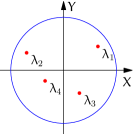
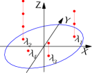
(a) (b) (c)

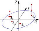
Figure 8. Classical spectrum of the matrix from the Ex. 4.9 is shown at (a). Covariant spectrum of the same matrix in the jet space is drawn at (b). The image of the covariant spectrum under the map from Ex. 4.11 is presented (c).

Example 4.9.

Let $J_{k}(\lambda)$ denote the Jordan block of the length $k$ for the eigenvalue $\lambda$. On the Fig. 8 there are two pictures of the spectrum for the matrix

$$a=J_{3}\left(\lambda_{1}\right)\oplus J_{4}\left(\lambda_{2}\right)\oplus J_{1}\left(\lambda_{3}\right)\oplus J_{2}\left(\lambda_{4}\right),$$

where

$$\lambda_{1}=\frac{3}{4}e^{i\pi/4},\quad\lambda_{2}=\frac{2}{3}e^{i5\pi/6},\quad\lambda_{3}=\frac{2}{5}e^{-i3\pi/4},\quad\lambda_{4}=\frac{3}{5}e^{-i\pi/3}.$$

Part (a) represents the conventional two-dimensional image of the spectrum, i.e. eigenvalues of $a$, and (b) describes spectrum $\mathbf{sp}\,{}a$ arising from the wavelet construction. The first image did not allow to distinguish $a$ from many other essentially different matrices, e.g. the diagonal matrix

$$\mathop{\operator@font diag}\nolimits\left(\lambda_{1},\lambda_{2},\lambda_{3},\lambda_{4}\right),$$

which even have a different dimensionality. At the same time the Fig. 8(b) completely characterise $a$ up to a similarity. Note that each point of $\mathbf{sp}\,a$ on Fig. 8(b) corresponds to a particular root vector, which spans a primary subrepresentation.

4.5. Spectral Mapping Theorem

As was mentioned in the Introduction a resonable spectrum should be linked to the corresponding functional calculus by an appropriate spectral mapping theorem. The new version of spectrum is based on prolongation of $\rho_{1}$ into jet spaces (see Section 4.3). Naturally a correct version of spectral mapping theorem should also operate in jet spaces.

Let $\phi:\mathbb{D}{}\rightarrow\mathbb{D}{}$ be a holomorphic map, let us define its action on functions $[\phi_{*}f](z)=f(\phi(z))$. According to the general formula (4.7) we can define the prolongation $\phi_{*}^{(n)}$ onto the jet space $\mathbb{J}^{n}{}$. Its associated action $\rho_{1}^{k}\phi_{*}^{(n)}=\phi_{*}^{(n)}\rho_{1}^{n}$ on the pairs $(\lambda,k)$ is given by the formula:

(4.8) $$\phi_{*}^{(n)}(\lambda,k)=\left(\phi(\lambda),\left[\frac{k}{\deg_{\lambda}\phi}\right]\right),$$

where $\deg_{\lambda}\phi$ denotes the degree of zero of the function $\phi(z)-\phi(\lambda)$ at the point $z=\lambda$ and $[x]$ denotes the integer part of $x$.

Theorem 4.10 (Spectral mapping).

Let $\phi$ be a holomorphic mapping $\phi:\mathbb{D}{}\rightarrow\mathbb{D}{}$ and its prolonged action $\phi_{*}^{(n)}$ defined by (4.8), then

$$\mathbf{sp}\,\phi(a)=\phi_{*}^{(n)}\mathbf{sp}\,a.$$

The explicit expression of (4.8) for $\phi_{*}^{(n)}$, which involves derivatives of $\phi$ upto $n$th order, is known, see for example [HornJohnson94, Thm. 6.2.25], but was not recognised before as form of spectral mapping.

Example 4.11.

Let us continue with Example 4.9. Let $\phi$ map all four eigenvalues $\lambda_{1}$, …, $\lambda_{4}$ of the matrix $a$ into themselves. Then Fig. 8(a) will represent the classical spectrum of $\phi(a)$ as well as $a$.

However Fig. 8(c) shows mapping of the new spectrum for the case $\phi$ has orders of zeros at these points as follows: the order $1$ at $\lambda_{1}$, exactly the order $3$ at $\lambda_{2}$, an order at least $2$ at $\lambda_{3}$, and finally any order at $\lambda_{4}$.

5. Open Problems

In this section we indicate several directions for further work which go through three main areas described in the paper..

5.1. Geometry

Geometry is most elaborated area so far, yet many directions are waiting for further exploration.

1. Möbius transformations (1.1) with three types of imaginary units appear from the action of the group $SL_{2}{}(\mathbb{R}{})$ on the homogeneous space $SL_{2}{}(\mathbb{R}{})/H$ [Kisil09c], where $H$ is any subgroup $A$, $N$, $K$ from the Iwasawa decomposition (1.3). Which other actions and hypercomplex numbers can be obtained from semisimple Lie groups and their subgroups?

2. Lobachevsky geometry of the upper half-plane is extremely beautiful and well-developed subject [Beardon05a] [CoxeterGreitzer]. However the traditional study is limited to one subtype out of nine possible: with the complex numbers for Möbius transformation and the complex imaginary unit used in FSCc (2.2). The remaining eight cases shall be explored in various directions, notably in the context of discrete subgroups [Beardon95].

3. The Filmore-Springer-Cnops construction, see subsection 2.2, is closely related to the orbit method [Kirillov99] applied to $SL_{2}{}(\mathbb{R}{})$. An extension of the orbit method from the Lie algebra dual to matrices representing cycles may be fruitful for semisimple Lie groups.

5.2. Analytic Functions

It is known that in several dimensions there are different notions of analyticity, e.g. several complex variables and Clifford analysis. However, analytic functions of a complex variable are usually thought to be the only options in a plane domain. The following seems to be promising:

1. Development of the basic components of analytic function theory (the Cauchy integral, the Taylor expansion, the Cauchy-Riemann and Laplace equations, etc.) from the same construction and principles in the elliptic, parabolic and hyperbolic cases and subcases.

2. Identification of Hilbert spaces of analytic functions of Hardy and Bergman types, investigation of their properties. Consideration of the corresponding Töplitz operators and algebras generated by them.

3. Application of analytic methods to elliptic, parabolic and hyperbolic equations and corresponding boundary and initial values problems.

4. Generalisation of the results obtained to higher dimensional spaces. Detailed investigation of physically significant cases of three and four dimensions.

5.3. Functional Calculus

The functional calculus of a finite dimensional operator considered in Section 4 is elementary but provides a coherent and comprehensive treatment. It shall be extended to further cases where other approaches seems to be rather limited.

1. Nilpotent and quasinilpotent operators have the most trivial spectrum possible (the single point $\{0\}$) while their structure can be highly non-trivial. Thus the standard spectrum is insufficient for this class of operators. In contract, the covariant calculus and the spectrum give complete description of nilpotent operators—the basic prototypes of quasinilpotent ones. For quasinilpotent operators the construction will be more complicated and shall use analytic functions mentioned in 5.2.i.

2. The version of covariant calculus described above is based on the discrete series representations of $SL_{2}{}(\mathbb{R}{})$ group and is particularly suitable for the description of the discrete spectrum (note the remarkable coincidence in the names).

   It is interesting to develop similar covariant calculi based on the two other representation series of $SL_{2}{}(\mathbb{R}{})$: principal and complementary [Lang85]. The corresponding versions of analytic function theories for principal [Kisil97c] and complementary series [Kisil05a] were initiated within a unifying framework. The classification of analytic function theories into elliptic, parabolic, hyperbolic [Kisil05a, Kisil06a] hints the following associative chains:

   Representations of $SL_{2}{}(\mathbb{R}{})$ —	Function Theory —	Type of Spectrum
   discrete series —	elliptic —	discrete spectrum
   principal series —	hyperbolic —	continuous spectrum
   complementary series —	parabolic —	residual spectrum

3. Let $a$ be an operator with $\mathbf{sp}\,a\in\bar{\mathbb{D}{}}$ and $\left\|a^{k}\right\|<Ck^{p}$. It is typical to consider instead of $a$ the power bounded operator $ra$, where $0<r<1$, and consequently develop its $H_{\infty}{}$ calculus. However such a regularisation is very rough and hides the nature of extreme points of $\mathbf{sp}\,{a}$. To restore full information a subsequent limit transition $r\rightarrow 1$ of the regularisation parameter $r$ is required. This make the entire technique rather cumbersome and many results have an indirect nature.

   The regularisation $a^{k}\rightarrow a^{k}/k^{p}$ is more natural and accurate for polynomially bounded operators. However it cannot be achieved within the homomorphic calculus Defn. 4.1 because it is not compatible with any algebra homomorphism. Albeit this may be achieved within the covariant calculus Defn. 4.4 and Bergman type space from 5.2.ii.

4. Several non-commuting operators are especially difficult to treat with functional calculus Defn. 4.1 or a joint spectrum. For example, deep insights on joint spectrum of commuting tuples [JTaylor72] refused to be generalised to non-commuting case so far. The covariant calculus was initiated [Kisil95i] as a new approach to this hard problem and was later found useful elsewhere as well. Multidimensional covariant calculus [Kisil04d] shall use analytic functions described in 5.2.iv.

5.4. Quantum Mechanics

Due to the space restrictions we did not mentioned connections with quantum mechanics [Kisil96a] [Kisil02e] [Kisil05c] [Kisil04a] [Kisil09a] [Kisil10a]. In general Erlangen approach is much more popular among physicists rather than mathematicians. Nevertheless its potential is not exhausted even there.

1. There is a possibility to build representation of the Heisenberg group using characters of its centre with values in dual and double numbers rather than in complex ones. This will naturally unifies classical mechanics, traditional QM and hyperbolic QM [Khrennikov08a].

2. Representations of nilpotent Lie groups with multidimensional centres in Clifford algebras as a framework for consistent quantum filed theories based on De Donder–Weyl formalism [Kisil04a].

Remark 5.1.

This work is performed within the “Erlangen programme at large” framework [Kisil06a, Kisil05a], thus it would be suitable to explain the numbering of various papers. Since the logical order may be different from chronological one the following numbering scheme is used:

Prefix	Branch description
“0” or no prefix	Mainly geometrical works, within the classical field of Erlangen programme by F. Klein, see  [Kisil05a] [Kisil09c]
“1”	Papers on analytical functions theories and wavelets, e.g. [Kisil97c]
“2”	Papers on operator theory, functional calculi and spectra, e.g. [Kisil02a]
“3”	Papers on mathematical physics, e.g. [Kisil10a]

For example, this is the first paper in the mathematical physics area.