Tunneling spectra of strongly coupled superconductors: Role of dimensionality

Abstract

We investigate numerically the signatures of collective modes in the tunneling spectra of superconductors. The larger strength of the signatures observed in the high-$T_{c}$ superconductors, as compared to classical low-$T_{c}$ materials, is explained by the low dimensionality of these layered compounds. We also show that the strong-coupling structures are dips (zeros in the $d^{2}I/dV^{2}$ spectrum) in $d$-wave superconductors, rather than the steps (peaks in $d^{2}I/dV^{2}$) observed in classical $s$-wave superconductors. Finally we question the usefulness of effective density of states models for the analysis of tunneling data in $d$-wave superconductors.

I Introduction

Many experiments have shown that the electrons in cuprate high-$T_{c}$ superconductors (HTS) are significantly renormalized by the interaction with collective modes. This renormalization appears in photoemission measurements as velocity changes in the quasi-particle dispersion (the “kinks”) accompanied by a drop of the quasi-particle life-time Damascelli et al. (2003); Campuzano et al. (2004). In tunneling, the renormalization shows up as a depression, or “dip”, in the $dI/dV$ curve with the associated nearby accumulation of spectral weight (the “hump”) Fischer et al. (2007). Similar signatures observed by tunneling spectroscopy in classical superconductors were successfully explained by the strong-coupling theory of superconductivity Eliashberg (1960); Schrieffer (1964); Carbotte (1990). There are, however, two striking differences between the structures observed in the cuprates and in low-$T_{c}$ metals such as Pb or Hg. The dip in the cuprates is electron-hole asymmetric, being strongest at negative bias, while no such asymmetry is seen in lead. The electron-hole asymmetry of the dip is due to the electron-hole asymmetry of the underlying electronic density of states (DOS) Eschrig and Norman (2000); Levy de Castro et al. (2008). Second, while the structures are subtle in low-$T_{c}$ materials—they induce a change smaller than 5% in the tunneling spectrum—the cuprate dip is generally a strong effect which, for instance, can reach $20\%$ in optimally doped Bi₂Sr₂Ca₂Cu₃O_10+δ (Bi-2223) Kugler et al. (2006). It is tempting to attribute this difference of intensities to a difference in the overall coupling strength, as suggested by the largely different $T_{c}$ values. However, a comparison of the effective masses indicates that the couplings are not very different in Pb where Swihart et al. (1965) $m^{*}/m=2.1$ and in the Bi-based cuprates where $m^{*}/m$ varies between $1.5$ and $3$ as a function of doping Johnson et al. (2001); Hwang et al. (2007). Here we show that the large magnitude of the dip feature results from the low dimensionality of the materials and the associated singularities in the electronic DOS.

Tunneling experiments in strongly coupled classical superconductors have been interpreted using a formalism Schrieffer et al. (1963) that neglects the momentum dependence of the Eliashberg functions and of the tunneling matrix element, and further assumes that the normal-state DOS $N_{0}(\omega)$ is constant over the energy range of interest. The tunneling conductance, then, only depends on the gap function $\Delta(\omega)$, whose energy variation reflects the singularities of the phonon spectrum Scalapino and Anderson (1964); McMillan and Rowell (1965). The dimensionality of the materials does not enter in this formalism. The effect of a non-constant $N_{0}(\omega)$ on the gap function has been discussed in the context of the A15 compounds Pickett (1980). However the direct effect of a rapidly varying $N_{0}(\omega)$ on the tunneling conductance became apparent only recently in the high-$T_{c}$ compounds Hoogenboom et al. (2003); Levy de Castro et al. (2008); Pir , and requires to go beyond the formalisms of Refs Schrieffer et al., 1963 and Pickett, 1980. In particular, one can no longer assume that the tunneling conductance is proportional to the product of the normal-state DOS by the “effective superconducting DOS” Schrieffer et al. (1963) $\text{Re}\big{[}|\omega|/\sqrt{\omega^{2}-\Delta^{2}(\omega)}\big{]}$, so that nothing justifies a priori to normalize the low-temperature tunneling conductance by the normal-state conductance as was done with low-$T_{c}$ superconductors.

Among the new approaches introduced to study strong-coupling effects in HTS, some have focused on generalizing the classical formalism to the case of $d$-wave pairing Abanov and Chubukov (2000); Zasadzinski et al. (2003); Chubukov and Norman (2004); Sandvik et al. (2004), still overlooking the dimensionality. Other models are strictly two dimensional (2D) and pay attention to the full electron dispersion Eschrig and Norman (2000); Hoogenboom et al. (2003); Devereaux et al. (2004); Zhu et al. (2006); Levy de Castro et al. (2008); Onufrieva and Pfeuty (2009), taking into account the singularities of $N_{0}(\omega)$. Most of these studies assume that the collective mode responsible for the strong-coupling signatures is the sharp $(\pi,\pi)$ spin resonance common to all cuprates near 30–50 meV (Ref. Sidis et al., 2004), but a phonon scenario was also put forward Devereaux et al. (2004); Sandvik et al. (2004). In the present work, we extend these approaches to three dimensions (3D) by means of an additional hopping $t_{z}$ describing the dispersion along the $c$ axis, and we study the evolution of the strong-coupling features in the tunneling spectrum along the 2D to 3D transition on increasing $t_{z}$. For simplicity we restrict to the spin-resonance scenario; the electron-phonon model can be treated along the same lines, and both models lead to the same main conclusions. The model we use is described in Sec. II, results are presented and discussed in Sec. III, and Sec. IV is devoted to investigating the validity and usefulness of the effective superconducting DOS concept.

II Model and method

Following previous works Hoogenboom et al. (2003); Levy de Castro et al. (2008); Jenkins et al. (2009) we assume that the differential conductance measured by a scanning tunneling microscope (STM) is proportional to the thermally-broadened local density of states (LDOS) at the tip apex Tersoff and Hamann (1983); Chen (1990), and that furthermore the energy dependence of the LDOS just outside the sample follows the energy dependence of the bulk DOS $N(\omega)$:

$$\frac{dI}{dV}\propto\int d\omega\,[-f^{\prime}(\omega-eV)]N(\omega),$$ (1)

where $f^{\prime}$ is the derivative of the Fermi function. In STM experiments, various sources of noise may contribute to broaden $N(\omega)$ further; when comparing theory and experiment we shall take these into account by a phenomenological Gaussian broadening.

In the superconducting state, the interaction with longitudinal spin fluctuations is described by the $2\times 2$ Nambu matrix self-energy,

$$\hat{\Sigma}(\bm{k},\omega)=-\frac{1}{\mathscr{N}}\sum_{\bm{q}}\frac{1}{\beta}\sum_{i\Omega_{n}}\,g^{2}\chi_{s}(\bm{q},i\Omega_{n})\times\\ \hat{G}_{0}(\bm{k}-\bm{q},i\omega_{n}-i\Omega_{n})\big{|}_{i\omega_{n}\to\omega+i0^{+}}$$ (2)

with $\chi_{s}$ the $\langle S^{z}S^{z}\rangle$ spin susceptibility, $g=\sqrt{3}\hbar J/2$ the coupling strength with $J$ the spin-spin interaction energy, and $\hat{G}_{0}$ the $2\times 2$ BCS matrix Green’s function. The sums extend over the $\mathscr{N}$ vectors $\bm{q}\equiv(\bm{q}_{\parallel},q_{z})$ in the three-dimensional Brillouin zone and the even Matsubara frequencies $i\Omega_{n}=2n\pi/\beta$ with $\beta=(k_{\text{B}}T)^{-1}$. Equation (2) gives the lowest-order term of an expansion in $J$ self-consistency . We follow Ref. Eschrig and Norman, 2000 and use for $\chi_{s}$ a model inspired by neutron-scattering experiments on the high-$T_{c}$ compounds. In this model, $\chi_{s}$ has no $q_{z}$ dependence and is the product of a Lorentzian peak centered at $(\pi,\pi)$ in the 2D Brillouin zone and another Lorentzian peak centered at the resonance energy $\Omega_{\text{sr}}$. The widths of the peaks are $\Delta q$ in momentum space and $\Gamma_{\text{sr}}$ in energy. This simple separable form of $\chi_{s}$ allows to evaluate analytically the frequency sum in Eq. (2), and to perform analytically the continuation from the odd frequencies $i\omega_{n}=(2n+1)\pi/\beta$ to the real-frequency axis. The remaining momentum integral is a convolution which can be efficiently performed using fast Fourier transforms. Also, the absence of $q_{z}$ dependence in $\chi_{s}$ implies that the self-energy does not depend on $k_{z}$. We use a BCS Green’s function broadened by a small phenomenological scattering rate $\Gamma$,

$$\hat{G}_{0}(\bm{k},i\omega_{n})=\frac{[i\omega_{n}+i\Gamma(i\omega_{n})]\hat{\tau}_{0}+\xi_{\bm{k}}\hat{\tau}_{3}+\Delta_{\bm{k}_{\parallel}}\hat{\tau}_{1}}{[i\omega_{n}+i\Gamma(i\omega_{n})]^{2}-\xi_{\bm{k}}^{2}-\Delta_{\bm{k}_{\parallel}}^{2}},$$ (3)

where $\Gamma(i\omega_{n})=\Gamma\,\text{sign}(\text{Im}\,i\omega_{n})$, $\hat{\tau}_{i}$ are the Pauli matrices with $\hat{\tau}_{0}$ the identity, and $\Delta_{\bm{k}_{\parallel}}=\Delta_{0}(\cos k_{x}-\cos k_{y})/2$ is the $d$-wave gap which we assume $k_{z}$ independent for simplicity. The additional effects resulting from a possible weak modulation Rajagopal and Jha (1996); Pairor (2005) of the gap along $k_{z}$ will be discussed toward the end of Sec. III. We do not address here the origin of the pairing leading to the BCS gap $\Delta_{\bm{k}_{\parallel}}$. With the high-$T_{c}$ compounds in mind, we consider a one-band model of quasi-2D electrons with a normal-state dispersion,

$$\xi_{\bm{k}}=\xi_{\bm{k}_{\parallel}}+2t_{z}\cos(k_{z}c),$$ (4)

where $\xi_{\bm{k}_{\parallel}}=\varepsilon_{\bm{k}_{\parallel}}-\mu$, $\mu$ being the chemical potential and $\varepsilon_{\bm{k}_{\parallel}}$ a five-neighbor tight-binding model on the square lattice ($a\equiv 1$), $\varepsilon_{\bm{k}_{\parallel}}=2t_{1}(\cos k_{x}+\cos k_{y})+4t_{2}\cos k_{x}\cos k_{y}+2t_{3}(\cos 2k_{x}+\cos 2k_{y})+4t_{4}(\cos 2k_{x}\cos k_{y}+\cos k_{x}\cos 2k_{y})+4t_{5}\cos 2k_{x}\cos 2k_{y}$.

The momentum dependence of the self-energy in Eq. (2) is not small (see, e.g., Fig. 1 of Ref. Eschrig and Norman, 2000 and Fig. 2 below). This is a major difference with respect to the electron-phonon models describing low-$T_{c}$ three-dimensional metals, where the momentum dependence of the self-energy can be neglected. The calculation of the DOS is therefore much more demanding since two three-dimensional momentum integrations must be performed for every energy $\omega$. The DOS is given by

$$N(\omega)=\frac{1}{\mathscr{N}}\sum_{\bm{k}}\left({\textstyle-\frac{1}{\pi}}\right)\text{Im}\,\hat{G}_{11}(\bm{k},\omega),$$ (5)

where $\hat{G}_{11}$ is the first component of the matrix $\hat{G}(\bm{k},\omega)=[\hat{G}^{-1}_{0}(\bm{k},\omega)-\hat{\Sigma}(\bm{k},\omega)]^{-1}$. In Eq. (5), the $k_{z}$ integration can be performed analytically (see Appendix) but not in Eq. (2). In order to achieve a good accuracy when computing the DOS $N(\omega)$, we evaluate the self-energy using a $2048\times 2048\times 256$ mesh in momentum space and a value $\Gamma=0.5$ meV. For the evaluation of the tunneling conductance $\Gamma$ is increased to 2 meV, which allows to decrease the mesh size to $1024\times 1024\times 256$.

The model in Eqs. (1)–(5) has several parameters but our focus is on the $c$-axis hopping energy $t_{z}$. In HTS, $t_{z}$ is not larger than a few meV, and setting it to zero seems appropriate to discuss tunneling data. Indeed, in the 2D limit the model was found to fit the experimental data for optimally doped Bi-2223 very well Levy de Castro et al. (2008); Jenkins et al. (2009). Here we take the parameters determined from one such fit as a starting point, and we vary $t_{z}$ to demonstrate the role of the dimensionality on the tunneling spectrum. The band parameters $t_{1\ldots 5}$ are $-200$, $31$, $-16$, $8$, and $-7$ meV, and the chemical potential is $\mu=-200$ meV. The gap magnitude is $\Delta_{0}=46$ meV. The spin-resonance energy is $\Omega_{\text{sr}}=34$ meV, its energy width $\Gamma_{\text{sr}}=2$ meV, and its momentum width $\Delta q=1.6a^{-1}$. Finally the coupling strength is $g=775$ meV, which implies a quasi-particle residue $Z=0.44$ and a mass renormalization $m^{*}/m=2.32$ at the nodal point of the Fermi surface. The temperature is set to $T=2$ K unless stated otherwise. The resulting theoretical tunneling conductance for $t_{z}=0$ is compared with experimental data in Fig. 1c (topmost curve).

III Results

The evolution of $N(\omega)$ with increasing $t_{z}$ is displayed in Fig. 1a. In the 2D limit, the DOS shows sharp and particle-hole asymmetric coherence peaks, strong and asymmetric dips, as well as humps and shoulders where the spectral weight expelled from the dips is accumulated. This produces, in particular, a characteristic widening of the coherence peaks basis, which becomes triangular. The particle-hole asymmetries reflect the particle-hole asymmetry of the corresponding bare DOS $N_{0}(\omega)$ shown in Fig. 1b, whose Van Hove singularity (VHS) lies slightly below $E_{\text{F}}$ at $-16$ meV: on the one hand, the spectral weight of the VHS goes to a larger degree into the negative-energy coherence peak, and on the other hand the enhancement of the scattering rate due to the VHS is stronger at negative energy, explaining the stronger dip at $\omega<0$ Eschrig and Norman (2000); Levy de Castro et al. (2008). This can also be seen in Fig. 2 where the electron-scattering rate $-\text{Im}\,\hat{\Sigma}_{11}(\bm{k},\omega)$ is displayed for the nodal and anti nodal points of the Fermi surface. The scattering rate vanishes for $|\omega|<\Omega_{\text{sr}}$ and has a pronounced, particle-hole asymmetric maximum near $|\omega|=\Omega_{\text{sr}}+\Delta_{0}$ (more precisely between $\Omega_{\text{sr}}+\Delta_{0}$ and $\Omega_{\text{sr}}+[\xi_{(\pi,0)}^{2}+\Delta_{0}^{2}]^{1/2}$). It is also clear from the figure that the energy of the scattering-rate peak shows no dispersion with momentum Eschrig and Norman (2000) but its intensity is strongly momentum dependent and larger by a factor $\sim 2.5$ in the anti nodal region as compared to the nodal region.

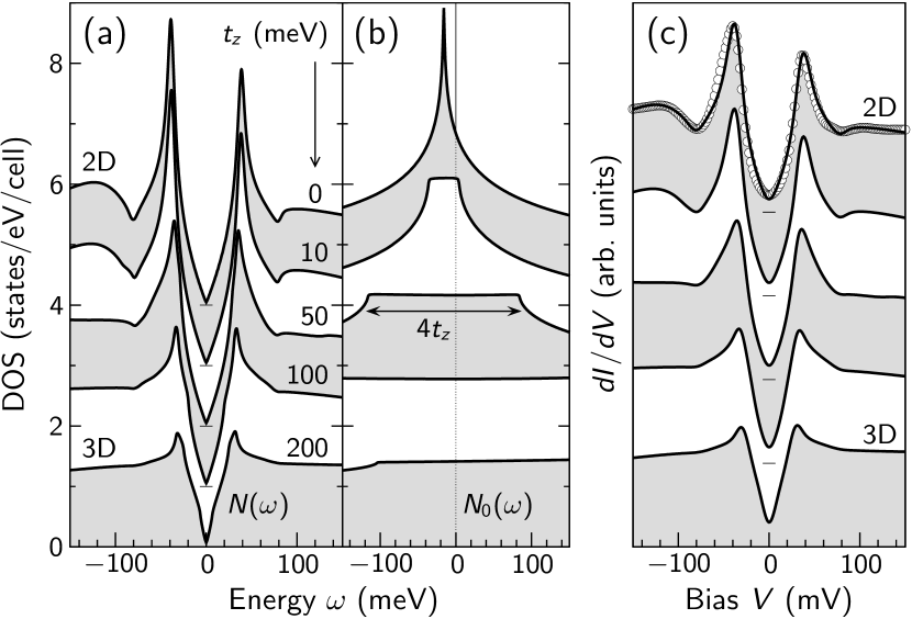
Figure 1: (a) Density of states $N(\omega)$ for superconducting electrons coupled to a $(\pi,\pi)$ spin resonance, as a function of the $c$-axis hopping $t_{z}$. For $t_{z}=0$, the system is two dimensional while for $t_{z}=200$ meV, it is three dimensional. (b) Normal-state bare DOS $N_{0}(\omega)$ for the same $t_{z}$ values. (c) Tunneling conductance for the same $t_{z}$ values. The temperature is $T=2$ K and a Gaussian broadening of 4 meV has been applied. The circles show the experimental data of Ref. Levy de Castro et al., 2008 compared to the $t_{z}=0$ spectrum. The curves in (a), (b), and (c) are offset vertically for clarity.

For $t_{z}>0$, the logarithmic divergence in $N_{0}(\omega)$ is cut on the scale of $4t_{z}$ due to dispersion along the $c$ axis (Fig. 1b). No significant change in either $N(\omega)$ or $dI/dV$ is observed for $t_{z}=10$ meV. This value is an upper bound for the $c$-axis hopping energy in the cuprates, and the relative insensitivity of the DOS to a small $c$-axis dispersion justifies the use of two-dimensional models for these systems. At larger $t_{z}$ values, however, the suppression of the divergence in $N_{0}(\omega)$ induces a drop of the coherence peaks in $N(\omega)$ and $dI/dV$. This is a direct effect of dimensionality on the tunneling spectrum, which was overlooked in the conventional strong-coupling approaches of Refs Schrieffer et al., 1963 and Pickett, 1980. Simultaneously the peak in the scattering rate is also suppressed with increasing $t_{z}$ (Fig. 2), leading to a weakening of the dip feature in $N(\omega)$ and $dI/dV$. This is an indirect effect of dimensionality, that is only revealed in the strong-coupling signatures.

Figure 2: Scattering rate $-\text{Im}\,\hat{\Sigma}_{11}$ as a function of energy for several values of $t_{z}$ at (a) the nodal point $\bm{k}_{\parallel}\approx(0.41,0.41)\pi/a$ and (b) the anti nodal point $\bm{k}_{\parallel}\approx(1,0.05)\pi/a$ of the Fermi surface shown in the insets. Curves are offset vertically for clarity. The dashed vertical lines delimit the energy range $|\omega|<\Omega_{\text{sr}}$ where inelastic scattering by the spin resonance is forbidden. The dotted vertical lines indicate $\pm(\Omega_{\text{sr}}+\Delta_{0})$.

Figure 3: Partial BCS density of states in two (2D) and three (3D) dimensions. The thin solid lines show the contribution coming from the $(\pi,0)$ region of the two-dimensional Brillouin zone, shaded in black in the inset while the dashed lines show the contribution of the remainder of the zone (shaded in gray). The thick line is the total BCS DOS.

As Fig. 2 shows, increasing the dimension not only suppresses the peak at $\Omega_{\text{sr}}+\Delta_{0}$ in the scattering rate but it also reduces its momentum dependence. In 2D, this peak arises because the $\bm{q}$ sum in Eq. (2) is dominated by the saddle-point region near $\bm{k}_{\text{M}}\equiv(\pi,0)$ and $\bm{k}_{\text{M}^{\prime}}\equiv(0,\pi)$, where the spectral weight of the BCS Green’s function is largest—i.e., $\bm{k}_{\parallel}-\bm{q}_{\parallel}\approx\bm{k}_{\text{M},\text{M}^{\prime}}$. Hence the peak energy is determined chiefly by the BCS excitation energy at $\bm{k}_{\text{M},\text{M}^{\prime}}$, shifted by $\Omega_{\text{sr}}$ due to the convolution with the spin susceptibility, and the peak intensity is controlled by the momentum dependence of $\chi_{s}\big{(}\bm{k}_{\parallel}-\bm{k}_{\text{M},\text{M}^{\prime}},\Omega_{\text{sr}}\big{)}$, which is at maximum for $\bm{k}_{\parallel}=\bm{k}_{\text{M}^{\prime},\text{M}}$. The situation changes in 3D because the anti-nodal regions no longer dominate the spectral weight, as illustrated in Fig. 3. This figure displays the partial BCS density of states, i.e., the part of the BCS DOS originating from states close to the $(\pi,0)$ and equivalent points. While in the 2D limit, a region covering just 14% of the zone around $(\pi,0)$ provides 56% of the spectral weight for energies between $\Omega_{\text{sr}}$ and $\Omega_{\text{sr}}+\Delta_{0}$, its contribution is reduced to 21% in the 3D limit. Hence the scattering rate in 3D is nearly momentum independent and almost constant above $\Omega_{\text{sr}}+\Delta_{0}$. Finally, the 2D to 3D transition also suppresses the particle-hole asymmetry of the scattering rate. This again results from the disappearance of particle-hole asymmetry in the underlying bare DOS (Fig. 1b) and in the corresponding BCS DOS (Fig. 3). Thus the $k_{z}$ dispersion simultaneously defeats four players who contribute to make the strong-coupling signatures in the 2D high-$T_{c}$ superconductors distinctly different from those in 3D metals: the Van Hove singularity, the particle-hole asymmetry, the momentum dependence, and the strong scattering enhancement at $|\omega|\approx\Omega_{\text{sr}}+\Delta_{0}$, especially near $(\pi,0)$.

In the curves of Figs. 1a and 1c corresponding to the 3D limit, the strong-coupling signatures are barely visible. Their magnitude is $\sim 1$%, smaller than the $\sim 5$% value observed in Pb. The origin of this difference lies in the gap symmetry. In $d$-wave superconductors, the coherence peaks in the BCS DOS are weak logarithmic singularities Won and Maki (1994) while in $s$-wave superconductors, they are strong square-root divergences. The strength of the scattering-rate peak at $\Omega_{\text{sr}}+\Delta_{0}$, and consequently the strength of the dip in the DOS and tunneling spectrum, are determined by the strength of the coherence peaks in the BCS DOS, as is clear from Eq. (2). In the case of a $d$-wave superconductor, the coherence peaks are cut in 3D as compared to 2D (see Fig. 3) in the same way as the logarithmic VHS in Fig. 1b, resulting in the suppression of the scattering-rate enhancement at $\Omega_{\text{sr}}+\Delta_{0}$ in Fig. 2. (Note that, roughly speaking, the scattering rate is proportional to the BCS DOS shifted in energy by $\pm\Omega_{\text{sr}}$.) The suppression of the BCS coherence peaks with increasing dimension also occurs in $s$-wave superconductors, but with one difference: if, on the one hand, the part of the coherence-peak spectral weight coming from the VHS gets suppressed, on the other hand, the square-root gap-edge singularities persist in any dimension. Therefore, in $s$-wave superconductors the strong-coupling signatures remain clearly visible in 3D. This is illustrated in Fig. 4a. The 2D and 3D DOS curves of Fig. 1a are compared to the curves obtained for the corresponding $s$-wave model, i.e., with all parameters unchanged except the gap which is replaced by $\Delta_{\bm{k}_{\parallel}}\equiv\Delta_{0}=46$ meV. The changes are quite dramatic. The first effect to notice is a drastic reduction in the peak-to-peak gap $\Delta_{p}$ in the $s$-wave case: a consequence of the pair-breaking nature of the coupling Eq. (2) in the $s$-wave channel Annett (1990); endnote1 . Still, the strong-coupling signatures appear at the same energy $\Omega_{\text{sr}}+\Delta_{0}=80$ meV in both $d$ and $s$ wave, due to our choice of the lowest-order model $\hat{\Sigma}\propto\chi_{s}\hat{G}_{0}$ in Eq. (2). The second observation is that the strong-coupling signatures look like steps in the $s$-wave DOS, like in the classical superconductors Schrieffer et al. (1963), reflecting the asymmetric shape of the BCS $s$-wave coherence peaks. In contrast, the signatures appear as local minima in the $d$-wave DOS, because the coherence peaks of the $d$-wave BCS DOS are nearly symmetric about their maximum. In short, the strong-coupling features give an “inverted image” of the BCS coherence peaks Levy de Castro et al. (2008). An interesting consequence follows: while in $s$-wave superconductors, the strong-coupling structures correspond to peaks in the second-derivative $d^{2}I/dV^{2}$ spectrum, for a $d$-wave gap they correspond to zeros in the $d^{2}I/dV^{2}$ spectrum, as demonstrated in Fig. 4b. This conclusion applies equally to phonon models and calls for a reinterpretation of cuprate $d^{2}I/dV^{2}$ data in which peaks were assigned to phonon modes Lee et al. (2006); Zhao (2007). Finally, one sees from Fig. 4 that in 3D the signatures remain strong for an $s$-wave gap, for the reason explained above, while they have almost disappeared in the $d$-wave case.

Figure 4: (a) Comparison of the $d$-wave and $s$-wave DOS for $t_{z}=0$ (2D) and $t_{z}=200$ meV (3D). The thick lines show $N(\omega)$ as in Fig. 1a. The thin lines show $N(\omega)$ computed with an $s$-wave gap of the same magnitude $\Delta_{0}=46$ meV, and all other parameters unchanged. (b) Second-derivative tunneling spectrum, $d^{2}I/dV^{2}$, in the region of the strong-coupling signature at negative bias. In the $s$-wave case, there is a peak in $d^{2}I/dV^{2}$ close to the energy $\Omega_{\text{sr}}+\Delta_{0}$ while in the $d$-wave case, there is a sign change in 2D and no clear signature in 3D.

The previous discussion underlines the role of the BCS coherence peaks in the formation, strength, and shape of the strong-coupling signatures. More generally, for such signatures to occur there must be divergences (or at least pronounced maxima) in the non-interacting DOS. Peaks in the “bosonic” spectrum are not sufficient, although they are necessary. Indeed, phonon structures are absent from the normal-state spectra of classical superconductors McMillan and Rowell (1969) because the normal-state DOS is flat, in spite of the facts that the phonon spectrum and the electron-phonon coupling do not change significantly at $T_{c}$. In contrast, the normal-state DOS of 2D high-$T_{c}$ superconductors exhibits structures, either the pseudogap Fischer et al. (2007) or the bare VHS Pir . One can therefore expect to see strong-coupling features in the normal-state spectra of HTS, provided that the peaks in the bosonic spectrum subsist above $T_{c}$. Figure 5 (thin lines) shows the normal-state DOS implied by setting $\Delta_{0}=0$ in our model, keeping the other parameters fixed (including temperature). As expected sharp strong-coupling features remain in 2D at energies $\pm\Omega_{\text{sr}}$ and $\xi_{(\pi,0)}-\Omega_{\text{sr}}=-50$ meV while nothing but very weak structures subsist in 3D, signaling the onset of scattering at $\pm\Omega_{\text{sr}}$. Unfortunately it turns out that in the HTS the spin resonance is absent above $T_{c}$—or at least below the background level of neutron-scattering experiments Bourges et al. (2000). The normal state of Bi-2223 has not been investigated by neutron scattering so far but we may borrow information from the much studied YBa₂Cu₃O_6+x system (Y-123). In Y-123, the normal-state spin susceptibility preserves its separable form with independent momentum and energy variations Regnault et al. (1995). It is still centered at $(\pi,\pi)$ with a broad maximum at a characteristic temperature-dependent frequency $\Omega_{\text{sf}}\approx\Omega_{\text{sr}}$. For the purpose of illustrating the effect of a broad spin-fluctuations continuum on the normal-state tunneling spectrum, it is sufficient to use the same model as in the superconducting state but with the new parameter $\Gamma_{\text{sr}}=14$ meV endnote2 . The resulting DOS calculated at $T=200$ K is shown by the thick lines in Fig. 5. The strong-coupling signatures are almost washed out in 2D and completely in 3D. This is not due to the thermal broadening of Eq. (1), not included in the DOS $N(\omega)$, but mostly to the intrinsic temperature dependence of the self-energy in Eq. (2), and, to a lesser extent, to the broader spin response. Hence, if structures due to interaction with spin fluctuations are unlikely to show up in the normal state of HTS, those associated with the interaction with phonons may well be observable if the coupling is strong enough since this coupling will not change appreciably at $T_{c}$.

Figure 5: Normal-state DOS. The thin lines show the $T=2$ K DOS for $\Delta_{0}=0$; the thick lines show the $T=200$ K DOS for $\Delta_{0}=0$ and $\Gamma_{\text{sr}}=14$ meV (see text). All other parameters are as in Fig. 1a.

In the present study, we have overlooked a possible $k_{z}$ dependence of the BCS gap, retaining only the $k_{z}$ dependence of the bare dispersion. A weak modulation of the BCS gap along $k_{z}$ is expected in 3D systems Rajagopal and Jha (1996). As shown in Ref. Pairor, 2005, such a modulation has the effect of cutting the logarithmic coherence peaks on the scale of $2\Delta_{z}$, with $\Delta_{z}$ the amplitude of the gap modulation. This is similar to the effect of $t_{z}$ on the BCS coherence peaks, which are cut on a scale corresponding to the gap variation along the warped 3D Fermi surface, namely, $\sim\Delta_{0}t_{z}/4t_{1}$, as seen in Fig. 3. The expected effect of $\Delta_{z}$ on the scattering rate is also an additional broadening on top of the one produced by $t_{z}$, $\hat{G}_{0}$ being replaced by its $k_{z}$ average in Eq. (2). Therefore, we expect that the gap modulation along $k_{z}$ will contribute to suppress the coherence peaks and the strong-coupling features even further with increasing $t_{z}$, as compared to the results in Fig. 1.

Our results can be summarized as follows. The formation of clear strong-coupling structures in the tunneling conductance requires two ingredients: (A) at least one peak in the spectrum of collective excitations and (B) at least one peak in the non-interacting or superconducting DOS. In classical superconductors, (A) is provided by optical phonons and (B) is the asymmetric square-root singularity at the edge of the $s$-wave gap: strong-coupling features are asymmetric steps—peaks in the $d^{2}I/dV^{2}$ curve—and dimensionality plays no big role because (A) and (B) are present in any dimension. In the normal state, there is no signature because (B) is absent. In high-$T_{c}$ layered superconductors, (A) is provided by the spin resonance and (B) has two sources: (B1) the logarithmic Van Hove singularity in the bare DOS; (B2) the symmetric logarithmic singularities at the edge of the $d$-wave gap. Strong-coupling signatures appear as local minima—zeros in the $d^{2}I/dV^{2}$ curve—but they vanish with increasing dimensionality from 2D to 3D because (B1) and (B2) both get suppressed by the $c$-axis dispersion. In the normal state of two-dimensional HTS, (B2) is absent, leaving aside the question of the pseudogap but (B1) remains and strong-coupling signatures are thus expected unless (A) disappears at $T_{c}$. This is the case for the spin resonance but certainly not for phonons, leaving open the possibility that phonon structures might be observable in the normal-state tunneling spectra.

IV DOS and effective DOS

The conventional theory of electron tunneling into superconductors Schrieffer et al. (1963) leads to an equation identical to Eq. (1) for the tunneling conductance, except that the DOS $N(\omega)$ is replaced by an “effective tunneling DOS” $N_{T}(\omega)=N_{0}(0)\text{Re}\big{[}|\omega|/\sqrt{\omega^{2}-\Delta^{2}(\omega)}\big{]}$. $N_{0}(0)$ is the normal-state DOS at zero energy—$N_{0}(\omega)\equiv N_{0}(0)$ is assumed—and $\Delta(\omega)$ is the gap function. The latter must be understood as a Fermi-surface average of weakly momentum-dependent quantities, $\Delta(\omega)=\langle\Phi(\bm{k},\omega)/Z(\bm{k},\omega)\rangle_{\text{FS}}$ with $\Phi$ and $Z$ the Eliashberg pairing and renormalization functions. In the notation of Eq. (2), they read $Z(\bm{k},\omega)=1-[\hat{\Sigma}_{11}(\bm{k},\omega)+\hat{\Sigma}_{22}(\bm{k},\omega)]/(2\omega)$ and, for an $s$-wave gap $\Delta_{0}$, $\Phi(\bm{k},\omega)=\Delta_{0}+\hat{\Sigma}_{12}(\bm{k},\omega)$. In a $d$-wave superconductor, the Fermi-surface average of the gap $\Delta_{\bm{k}}$ vanishes, and so does the average of the off-diagonal self-energy since $\hat{\Sigma}_{12}(\bm{k},\omega)\propto\Delta_{\bm{k}}$. The effective tunneling DOS concept is logically generalized Abanov and Chubukov (2000); Zasadzinski et al. (2003) by writing $N_{T}(\omega)=N_{0}(0)\text{Re}\big{\langle}|\omega|/\sqrt{\omega^{2}-[\Delta_{\bm{k}}\phi(\omega)]^{2}}\big{\rangle}_{\text{FS}}$ with

$$\phi(\omega)=\left\langle\frac{1+\hat{\Sigma}_{12}(\bm{k},\omega)/\Delta_{\bm{k}}}{1-[\hat{\Sigma}_{11}(\bm{k},\omega)+\hat{\Sigma}_{22}(\bm{k},\omega)]/(2\omega)}\right\rangle_{\text{FS}}.$$ (6)

This form of $N_{T}(\omega)$ is an even function of $\omega$, and cannot fit the particle-hole asymmetric spectra in HTS. Therefore, a further generalization of the effective tunneling DOS has been necessary, namely,

$$N_{T}(\omega)=N_{0}(\omega)\,\text{Re}\left\langle\frac{|\omega|}{\sqrt{\omega^{2}-[\Delta_{\bm{k}}\phi(\omega)]^{2}}}\right\rangle_{\text{FS}}$$ (7)

which suggests that the “true” superconducting DOS can be obtained by dividing the tunneling spectrum in the superconducting state by the spectrum in the normal state Zasadzinski et al. (2003); Romano et al. (2006); Boyer et al. (2007); Pasupathy et al. (2008).

Equation (7) is very convenient, but lacks a formal justification. Our model offers the opportunity to investigate the usefulness of Eq. (7), by comparing numerically the actual tunneling DOS $N(\omega)$ of Eq. (5) with the effective tunneling DOS $N_{T}(\omega)$. For the practical evaluation of $N_{T}(\omega)$, we define the Fermi-surface average as

$$\left\langle\,\cdots\right\rangle_{\text{FS}}\equiv\frac{\sum_{\bm{k}}A_{0}(\bm{k},0)\,(\,\cdots)}{\sum_{\bm{k}}A_{0}(\bm{k},0)}$$ (8)

with $A_{0}(\bm{k},0)$ the zero-energy spectral function in the absence of pairing: $A_{0}(\bm{k},0)=(-1/\pi)\text{Im}\,\hat{G}_{11}(\bm{k},0)|_{\Delta_{\bm{k}}=0}$. With this definition, the average is performed on the renormalized Fermi surface, defined by $\xi_{\bm{k}}+\text{Re}\,\hat{\Sigma}_{11}(\bm{k},0)=0$, rather than the bare Fermi surface $\xi_{\bm{k}}=0$. Furthermore, each state gets correctly weighted if the spectral weight is unevenly distributed along the Fermi surface.

Figure 6: (Left panels) Real part (solid lines) and imaginary part (dashed lines) of the pairing function defined in Eq. (6) for $t_{z}=0$ (2D) and $t_{z}=200$ meV (3D). (Right panels) Comparison of the effective tunneling DOS $N_{T}(\omega)$ of Eq. (7) with the actual DOS $N(\omega)$ of Eq. (5). The dashed lines show $N_{T}(\omega)/N_{0}(\omega)$. In all graphs, the dotted vertical lines mark the energy $\pm(\Omega_{\text{sr}}+\Delta_{0})$.

A comparison of $N(\omega)$ and $N_{T}(\omega)$ is displayed in Fig. 6, where the pairing function $\phi(\omega)$ is also shown. In two dimensions, the real part of $\phi(\omega)$ has a maximum at $\omega=\Omega_{\text{sr}}+\Delta_{0}$, where its imaginary part shows a rapid variation. This is analogous to the behavior reported in Ref. Schrieffer et al., 1963. The resulting $N_{T}(\omega)$ also shows a behavior similar to the one found in Ref. Schrieffer et al., 1963: $N_{T}(\omega)$ is larger than the BCS density of states at energies smaller than $\Omega_{\text{sr}}+\Delta_{0}$ and drops below the BCS DOS at $\Omega_{\text{sr}}+\Delta_{0}$. The actual DOS $N(\omega)$, however, behaves differently: it is smaller than the BCS DOS between the coherence peak and some energy above the dip minimum (see also Fig. 1 of Ref. Levy de Castro et al., 2008). Thus, although the positions of the strong-coupling features are identical in $N_{T}(\omega)$ and $N(\omega)$, their shape is markedly different in 2D $d$-wave superconductors. In 3D, the difference between $N_{T}(\omega)$ and $N(\omega)$ is less severe than in 2D, and both curves show very weak signatures, although those in $N(\omega)$ are slightly stronger. Finally, the $N_{T}(\omega)$ curves show structures which are absent in the $N(\omega)$ curves. In 2D, a peak at $\omega=-16~{}\text{meV}=\xi_{(\pi,0)}$ appears due to the VHS in $N_{0}(\omega)$; this peak is unphysical because in the actual energy spectrum, the VHS is pushed to $-[\xi_{(\pi,0)}^{2}+\Delta_{0}^{2}]^{1/2}$. In 3D, $N_{T}(\omega)$ has a structure near $-100$ meV, which also comes from the bare DOS $N_{0}(\omega)$ as can be seen in Fig. 1b. In the actual spectrum, this structure is suppressed due to the persistence of a large scattering rate at energies much higher than the threshold $\Omega_{\text{sr}}$ (see Fig. 2). These problems illustrate the limitations of the simple product Ansatz Eq. (7) for analyzing the tunneling spectrum of $d$-wave superconductors.

Appendix: Analytical $k_{z}$ integration

If the Nambu self-energy has no $k_{z}$ dependence, the $k_{z}$ sum in Eq. (5) can be performed analytically. This is the case in our model defined in Eq. (2). Solving Dyson’s equation $\hat{G}(\bm{k},\omega)=[\hat{G}^{-1}_{0}(\bm{k},\omega)-\hat{\Sigma}(\bm{k},\omega)]^{-1}$ with $\hat{G}_{0}$ given by Eq. (3), we find

$$\hat{G}_{11}(\bm{k},\omega)=\frac{1}{\omega+i\Gamma-\xi_{\bm{k}}-\hat{\Sigma}_{11}(\bm{k},\omega)-[\Delta_{\bm{k}_{\parallel}}+\hat{\Sigma}_{12}(\bm{k},\omega)]^{2}\big{/}[\omega+i\Gamma+\xi_{\bm{k}}-\hat{\Sigma}_{22}(\bm{k},\omega)]}.$$ (9)

Since $\hat{\Sigma}$ does not depend on $k_{z}$ (although it does depend on $t_{z}$), the $k_{z}$ dependence only comes from $\xi_{\bm{k}}$ in Eq. (4) and we can make it explicit by rewriting

$$\hat{G}_{11}(\bm{k},\omega)=\frac{1}{z_{11}-2t_{z}\cos(k_{z}c)-z_{12}^{2}\big{/}[z_{22}+2t_{z}\cos(k_{z}c)]}\\ =\frac{1}{2}\left(1+\frac{\zeta}{\lambda}\right)\frac{1}{\eta+\lambda-2t_{z}\cos(k_{z}c)}+\frac{1}{2}\left(1-\frac{\zeta}{\lambda}\right)\frac{1}{\eta-\lambda-2t_{z}\cos(k_{z}c)}.$$ (10)

In Eq. (10), the quantities $z_{11}$, $z_{22}$, $z_{12}$, $\zeta$, $\lambda$, and $\eta$ are all functions of $\bm{k}_{\parallel}$ and $\omega$ but not of $k_{z}$. Explicitly, $z_{11}=\omega+i\Gamma-\xi_{\bm{k}_{\parallel}}-\hat{\Sigma}_{11}(\bm{k}_{\parallel},\omega)$, $z_{22}=\omega+i\Gamma+\xi_{\bm{k}_{\parallel}}-\hat{\Sigma}_{22}(\bm{k}_{\parallel},\omega)$, $z_{12}=\Delta_{\bm{k}_{\parallel}}+\hat{\Sigma}_{12}(\bm{k}_{\parallel},\omega)$, $\zeta=(z_{11}+z_{22})/2$, $\lambda=\sqrt{\zeta^{2}-z_{12}^{2}}$, and $\eta=(z_{11}-z_{22})/2$. The $k_{z}$ integration can then be performed by means of the identity,

$$\tilde{D}_{t}(z)\equiv\frac{1}{2\pi}\int_{-\pi}^{\pi}\frac{dx}{z-2t\cos x}=\frac{1}{\sqrt{z-2t}\sqrt{z+2t}}$$ (11)

and yields

$$N(\omega)=\frac{1}{\mathscr{N}_{\parallel}}\sum_{\bm{k}_{\parallel}}\left({\textstyle-\frac{1}{\pi}}\right)\text{Im}\,\left\{\frac{1}{2}\left(1+\frac{\zeta}{\lambda}\right)\tilde{D}_{t_{z}}(\eta+\lambda)+\right.\\ \left.\frac{1}{2}\left(1-\frac{\zeta}{\lambda}\right)\tilde{D}_{t_{z}}(\eta-\lambda)\right\},$$ (12)

where $\mathscr{N}_{\parallel}$ is the number of $\bm{k}_{\parallel}$ points in the 2D Brillouin zone.

References

- Damascelli et al. (2003) A. Damascelli, Z. Hussain, and Z.-X. Shen, Rev. Mod. Phys. 75, 473 (2003).
- Campuzano et al. (2004) J. C. Campuzano, M. Norman, and M. Randeria, in Physics of Superconductors, edited by K. H. Bennemann and J. B. Ketterson (Springer, Berlin, 2004), Vol. II, p. 167.
- Fischer et al. (2007) Ø. Fischer, M. Kugler, I. Maggio-Aprile, C. Berthod, and C. Renner, Rev. Mod. Phys. 79, 353 (2007).
- Eliashberg (1960) G. M. Eliashberg, Sov. Phys. JETP 11, 696 (1960).
- Schrieffer (1964) J. R. Schrieffer, Theory of Superconductivity (Benjamin, New York, 1964).
- Carbotte (1990) J. P. Carbotte, Rev. Mod. Phys. 62, 1027 (1990).
- Eschrig and Norman (2000) M. Eschrig and M. R. Norman, Phys. Rev. Lett. 85, 3261 (2000); Phys. Rev. B 67, 144503 (2003).
- Levy de Castro et al. (2008) G. Levy de Castro, C. Berthod, A. Piriou, E. Giannini, and Ø. Fischer, Phys. Rev. Lett. 101, 267004 (2008).
- Kugler et al. (2006) M. Kugler, G. Levy de Castro, E. Giannini, A. Piriou, A. A. Manuel, C. Hess, and Ø. Fischer, J. Phys. Chem. Solids 67, 353 (2006).
- Swihart et al. (1965) J. C. Swihart, D. J. Scalapino, and Y. Wada, Phys. Rev. Lett. 14, 106 (1965).
- Johnson et al. (2001) P. D. Johnson, T. Valla, A. V. Fedorov, Z. Yusof, B. O. Wells, Q. Li, A. R. Moodenbaugh, G. D. Gu, N. Koshizuka, C. Kendziora, S. Jian, and D. G. Hinks, Phys. Rev. Lett. 87, 177007 (2001).
- Hwang et al. (2007) J. Hwang, T. Timusk, E. Schachinger, and J. P. Carbotte, Phys. Rev. B 75, 144508 (2007).
- Schrieffer et al. (1963) J. R. Schrieffer, D. J. Scalapino, and J. W. Wilkins, Phys. Rev. Lett. 10, 336 (1963).
- Scalapino and Anderson (1964) D. J. Scalapino and P. W. Anderson, Phys. Rev. 133, A921 (1964).
- McMillan and Rowell (1965) W. L. McMillan and J. M. Rowell, Phys. Rev. Lett. 14, 108 (1965).
- Pickett (1980) W. E. Pickett, Phys. Rev. B 21, 3897 (1980).
- Hoogenboom et al. (2003) B. W. Hoogenboom, C. Berthod, M. Peter, Ø. Fischer, and A. A. Kordyuk, Phys. Rev. B 67, 224502 (2003).
- (18) A. Piriou, N. Jenkins, C. Berthod, I. Maggio-Aprile, and Ø. Fischer, to be published.
- Abanov and Chubukov (2000) A. Abanov and A. V. Chubukov, Phys. Rev. B 61, R9241 (2000).
- Zasadzinski et al. (2003) J. F. Zasadzinski, L. Coffey, P. Romano, and Z. Yusof, Phys. Rev. B 68, 180504(R) (2003).
- Chubukov and Norman (2004) A. V. Chubukov and M. R. Norman, Phys. Rev. B 70, 174505 (2004).
- Sandvik et al. (2004) A. W. Sandvik, D. J. Scalapino, and N. E. Bickers, Phys. Rev. B 69, 094523 (2004).
- Devereaux et al. (2004) T. P. Devereaux, T. Cuk, Z.-X. Shen, and N. Nagaosa, Phys. Rev. Lett. 93, 117004 (2004); T. Cuk, D. H. Lu, X. Z. Zhou, Z.-X. Shen, T. P. Devereaux, and N. Nagaosa, Phys. Status Solidi B 242, 11 (2005).
- Zhu et al. (2006) J.-X. Zhu, A. V. Balatsky, T. P. Devereaux, Q. Si, J. Lee, K. McElroy, and J. C. Davis, Phys. Rev. B 73, 014511 (2006).
- Onufrieva and Pfeuty (2009) F. Onufrieva and P. Pfeuty, Phys. Rev. Lett. 102, 207003 (2009).
- Sidis et al. (2004) Y. Sidis, S. Pailhès, B. Keimer, P. Bourges, C. Ulrich, and L. P. Regnault, Phys. Status Solidi B 241, 1204 (2004).
- Jenkins et al. (2009) N. Jenkins, Y. Fasano, C. Berthod, I. Maggio-Aprile, A. Piriou, E. Giannini, B. W. Hoogenboom, C. Hess, T. Cren, and Ø. Fischer, Phys. Rev. Lett. 103, 227001 (2009).
- Tersoff and Hamann (1983) J. Tersoff and D. R. Hamann, Phys. Rev. Lett. 50, 1998 (1983).
- Chen (1990) C. J. Chen, Phys. Rev. B 42, 8841 (1990).
- (30) In electron-phonon models, the Migdal argument allows to neglect vertex corrections and obtain an accurate self-consistent theory by replacing in the self-energy by the full (Refs Migdal, 1958 and McMillan and Rowell, 1969). As there is no such theorem for spin fluctuations, the self-consistent model is not necessarily better (i.e., closer to the exact result including all vertex corrections) than the lowest-order model . This issue has been pointed out in the case of the Hubbard model (Ref. Vilk and Tremblay, 1997), and is also well known in the context of the approximation for the long-range Coulomb interaction, where the self-consistent version often gives poorer results than the non self-consistent one (Ref. Hedin, 1999). The situation is further complicated if one uses a phenomenological spin susceptibility in Eq. (2), rather than the spin susceptibility calculated using a consistent approximation. No systematic inclusion of vertex corrections is possible in this latter case. Hence the justification of Eq. (2) and of the corresponding self-consistent model (Ref. Onufrieva and Pfeuty, 2009) resides in their ability to properly describe experiments.
- Migdal (1958) A. B. Migdal, Sov. Phys. JETP 7, 996 (1958).
- McMillan and Rowell (1969) W. L. McMillan and J. M. Rowell, in Superconductivity, edited by R. D. Parks (Dekker, New York, 1969), Vol. 1, p. 561.
- Vilk and Tremblay (1997) Y. M. Vilk and A.-M. S. Tremblay, J. Phys. I 7, 1309 (1997).
- Hedin (1999) L. Hedin, J. Phys.: Condens. Matter 11, R489 (1999).
- Rajagopal and Jha (1996) A. K. Rajagopal and S. S. Jha, Phys. Rev. B 54, 4331 (1996); S. S. Jha and A. K. Rajagopal, Phys. Rev. B 55, 15248 (1997).
- Pairor (2005) P. Pairor, Phys. Rev. B 72, 174519 (2005).
- Won and Maki (1994) H. Won and K. Maki, Phys. Rev. B 49, 1397 (1994).
- Annett (1990) J. F. Annett, Adv. Phys. 39, 83 (1990).
- (39) Just the opposite happens in electron-phonon models, which are pair breaking in the -wave channel. In electron-phonon models, the self-energy Eq. (2) is replaced by, schematically, with the electron-phonon coupling and the phonon propagator (Ref. Schrieffer, 1964). The matrices appear because phonons couple to the charge density—while spin fluctuations couple to the spin density, and they change the sign of the component controlling the gap renormalization.
- Lee et al. (2006) J. Lee, K. Fujita, K. McElroy, J. A. Slezak, M. Wang, Y. Aiura, H. Bando, M. Ishikado, T. Masui, J. X. Zhu, A. V. Balatsky, H. Eisaki, S. Uchida, and J. C. Davis, Nature 442, 546 (2006).
- Zhao (2007) Guo-meng Zhao, Phys. Rev. B 75, 214507 (2007).
- Bourges et al. (2000) P. Bourges, B. Keimer, L. P. Regnault, and Y. Sidis, J. Supercond. 13, 735 (2000).
- Regnault et al. (1995) L. P. Regnault, P. Bourges, P. Burlet, J. Y. Henry, J. Rossat-Mignod, Y. Sidis, and C. Vettier, Physica B 213-214, 48 (1995).
- (44) The 200 K data in Fig. 7 of Ref. Regnault et al., 1995 can be well fitted to the Lorentzian form used for the spin susceptibility in Eq. (2), namely, , with the parameters meV, meV, and . On the other hand, the momentum width of the spin response was found to be temperature independent. To model the normal state of Bi-2223, we may therefore keep fixed and increase to the value of meV. In the absence of more detailed information, we do not change the value of , which now plays the role of the broad maximum in the magnetic response. These new parameters lead to a reduced effective mass in the normal state as compared to the superconducting state.
- Romano et al. (2006) P. Romano, L. Ozyuzer, Z. Yusof, C. Kurter, and J. F. Zasadzinski, Phys. Rev. B 73, 092514 (2006).
- Boyer et al. (2007) M. C. Boyer, W. D. Wise, C. Kamalesh, M. Yi, T. Kondo, T. Takeuchi, H. Ikuta, and E. W. Hudson, Nat. Phys. 3, 802 (2007).
- Pasupathy et al. (2008) A. N. Pasupathy, A. Pushp, K. K. Gomes, C. V. Parker, J. Wen, Z. Xu, G. Gu, S. Ono, Y. Ando, and A. Yazdani, Science 320, 196 (2008).