Cross-Identification of Stars with Unknown Proper Motions

Abstract

The cross-identification of sources in separate catalogs is one of the most basic tasks in observational astronomy. It is, however, surprisingly difficult and generally ill-defined. Recently Budavári & Szalay (2008) formulated the problem in the realm of probability theory, and laid down the statistical foundations of an extensible methodology. In this paper, we apply their Bayesian approach to stars with detectable proper motion, and show how to associate their observations. We study models on a sample of stars in the Sloan Digital Sky Survey, which allow for an unknown proper motion per object, and demonstrate the improvements over the analytic static model. Our models and conclusions are directly applicable to upcoming surveys such as PanSTARRS, the Dark Energy Survey, Sky Mapper, and the LSST, whose data sets will contain hundreds of millions of stars observed multiple times over several years.

1. Introduction

At the heart of many astronomical studies today is the basic step of catalog merging; combining measurements from different time intervals, wavelengths, and potentially separate instruments and telescopes. Scientific analyses exploit these multicolor cross-matches to understand the temporal and photometric nature of the underlying objects. In doing so they rely implicitly on the quality of the associations, thus the cross-identification of sources is arguably one of the most important steps in measuring the properties of celestial objects.

In general, cross-matching catalogs is a difficult problem that cannot really be separated from the scientific question at hand. An example of this is apparent when we consider the case of stellar observations. Stars that move between observations, due to their proper motions, are difficult to merge into multicolor sources (even within a single survey). Yet without the multicolor information it might not be possible to classify the source as a star in the first place. With a new generation of surveys that will take large quantities of multicolor photometry covering the Galactic Plane and observed over a period of several years (e.g. the Panoramic Survey Telescope & Rapid Response System, PanSTARRS, and the Large Synoptic Survey Telescope, LSST) it is clear that addressing these issues is becoming a serious concern.

In the recent work of Budavári & Szalay (2008) a general probabilistic formalism was introduced that is extendable to arbitrarily complex models. The beauty of the approach of Bayesian hypothesis testing is that it clearly separates the contributions of different types of measurements, e.g., the position on the sky or the colors of the sources, yet, naturally combines them into a coherent method. It is a generic framework that provides the prescription for the calculations that can be refined with more and more sophisticated modeling.

In this paper, we go beyond the simple case of stationary objects, and study the cross-identification of point sources that move on the sky. Most importantly we focus on stars that can be significantly offset between the epochs of observations. Although we only have loose constraints on their proper motions in general, this prior knowledge is enough to revise our static models, and work out the Bayesian evidence of the matches. In Section 2 we introduce a class of models that allow for changes in the position over time. Section 3 deals with the a priori constraints on the proper motions of the stars and their empirical ensemble statistics. In Section 4 we show the improvements over the static model on actual observations of stars, and Section 5 concludes our study. Throughout this paper, we adopt the convention to use the capital $P$ symbol for probabilities and the lower case $p$ letter for probability densities.

2. Proper Motion

Conceptually, modeling the position of moving sources is straightforward. The description combines the motion and the uncertainty of the astrometric measurements. The first question to answer is where on the sky one should expect to see an object of a certain proper motion, if it had been in some known position at a given time. Next, we calculate the evidence that given detections are truly observations of the same object.

2.1. Multi-epoch Models

The positional accuracy is characterized by a probability density function (hereafter PDF) on the celestial sphere. In a given model $M$, this $p(\mbox{\boldmath{$x$}}|\mbox{\boldmath{$r$}},M)$ function tells us where to expect $x$ detections of an object that is at its true location $r$. Throughout this paper, we use 3-dimensional unit vectors for the positions on the sky, e.g., the aforementioned $x$ and $r$ quantities. Usually the PDF is a very sharp peak and is assumed to be a normal distribution with some angular accuracy $\sigma$. The correct generalization to directional measurements is the Fisher (1953) distribution,

$$F(\mbox{\boldmath{$x$}}|\mbox{\boldmath{$r$}},w)=\frac{w\,\delta(|\mbox{\boldmath{$x$}}|\!-\!1)}{4\pi\sinh w}\ \exp\left({w\,\mbox{\boldmath{$r$}}{}\mbox{\boldmath{$x$}}}\right)$$ (1)

whose shape parameter $w$ is essentially $1/\sigma^{2}$ in the limit of large concentration; see details in Budavári & Szalay (2008).

The added complication comes from the fact that some objects are not stationary. If a given star is at location $r$ now and has $\mu$ proper motion then $\Delta{}t$ time later, it would be at some other position $\mbox{\boldmath{$r$}}^{\prime}$

$$\mbox{\boldmath{$r$}}^{\prime}=\mbox{\boldmath{$r$}}^{\prime}(\Delta{}t;\mbox{\boldmath{$r$}},\mbox{\boldmath{$\mu$}})$$ (2)

that is offset by a small displacement along a great circle. By substituting this position into our astrometric model, we create a new one $M^{\prime}$ with the added proper motion, $\mu$, and time difference, $\Delta{}t$, parameters.

$$p(\mbox{\boldmath{$x$}}|\Delta{}t,\mbox{\boldmath{$r$}},\mbox{\boldmath{$\mu$}},M^{\prime})=F\left(\mbox{\boldmath{$x$}}|\mbox{\boldmath{$r$}}^{\prime}(\Delta{}t;\mbox{\boldmath{$r$}},\mbox{\boldmath{$\mu$}}),w\right)$$ (3)

Naturally, there is nothing specific in this about the chosen characterization of the astrometry; one can use any appropriate PDF in place of the Fisher distribution instead.

2.2. The Bayes Factor

At the heart of the probabilistic cross-identification is the Bayes factor used for hypothesis testing. The question we are asking is whether our data $D$, a set of detected sources in separate catalogs with positions $\{\mbox{\boldmath{$x$}}_{i}\}$, are truly from the same object. For every catalog, we know its epoch and its astrometry characterized by a known $p_{i}$ PDF. Let $H$ denote the hypothesis that assumes that all measured positions are observations of the same object, and let $K$ denote its complement, i.e., any one or more of the detections might belong to a separate object. By definition, the Bayes factor is the ratio of the likelihoods of the two hypotheses we wish to compare,

$$B(H,K|D) = \frac{p(D|H)}{p(D|K)}$$ (4)

that are calculated as the integrals over their entire parameter spaces.

If we assume that there is a single object behind the observations, we can integrate over its unknown proper motion and position to calculate

$$p(D|H)=\int\!\!\!d\mbox{\boldmath{$r$}}\!\!\int\!\!\!d\mbox{\boldmath{$\mu$}}\,p(\mbox{\boldmath{$r$}},\mbox{\boldmath{$\mu$}}|H)\prod_{i=1}^{n}p_{i}(\mbox{\boldmath{$x$}}_{i}|\Delta{}t_{i},\mbox{\boldmath{$r$}},\mbox{\boldmath{$\mu$}},H)$$ (5)

where the joint likelihood of $H$ given the data is written as the product of the independent components and $p(\mbox{\boldmath{$r$}},\mbox{\boldmath{$\mu$}})$ is the prior on the parameters, which is the subject of the following section. The actual calculation of this likelihood depends on the prior and might only be accessible via numerical methods.

The complementary hypothesis is more complicated in the sense that the model has a set of independent objects with $\{\mbox{\boldmath{$r$}}_{i},\mbox{\boldmath{$\mu$}}_{i}\}$ parameters, however, the result of the calculation turns out to be much simpler. Here the integral separates into the product of

$$p(D|K)=\prod_{i=1}^{n}\int\!\!\!d\mbox{\boldmath{$r$}}_{i}\!\!\int\!\!\!d\mbox{\boldmath{$\mu$}}_{i}\,p(\mbox{\boldmath{$r$}}_{i},\mbox{\boldmath{$\mu$}}_{i}|K)\,p_{i}(\mbox{\boldmath{$x$}}_{i}|\Delta{}t_{i},\mbox{\boldmath{$r$}}_{i},\mbox{\boldmath{$\mu$}}_{i},K)$$ (6)

For each integral, we can select a reference time such that $\Delta{}t_{i}=0$, hence the effect of the proper motion drops out, and we arrive at the same result as the stationary case discussed by Budavári & Szalay (2008).

3. Prior Determination

The proper motion really only shows up in the numerator of the Bayes factor for assessing the quality of the association. The model is well-defined but the integration domain is set by the joint prior that is yet to be determined. In general, the prior $p(\mbox{\boldmath{$r$}},\mbox{\boldmath{$\mu$}}|H)$ can be very complicated for its dependence on the properties of the star. Simply put, brighter sources are likely to be closer, and hence, have a larger proper motion. More complicated is the effect of the color that is (along with its magnitude) a proxy for placing the star in different stellar populations with different dynamics. In this paper, we will not discuss these effects that will be a topic of future work. We also note that the prior can be a function of the time difference, $\Delta t$, to account for cases when the star travels far between observations to a new location with different source density. However, we expect this to be a small effect because the typical speed of stars and the usual time differences between observations today yield small displacements on the sky.

Using the basic properties of conditional densities, we can write it as the product

$$p(\mbox{\boldmath{$r$}},\mbox{\boldmath{$\mu$}}|H)=p(\mbox{\boldmath{$r$}}|H)\,p(\mbox{\boldmath{$\mu$}}|\mbox{\boldmath{$r$}},H)$$ (7)

where the first term is the prior on the position, e.g., the all-sky prior written with Dirac’s $\delta$ symbol as

$$p(\mbox{\boldmath{$r$}}|H)=\frac{1}{4\pi}\,\delta(|\mbox{\boldmath{$r$}}|-1)$$ (8)

and the more complicated second term describes the possible proper motions as a function of location and optionally other properties. The simplest possible model, after the stationary case, is to assume a uniform prior on $\mu$ up to some $\mu_{\rm{max}}$ limit independent of the location, i.e.,

$$p(\mbox{\boldmath{$\mu$}}|\mbox{\boldmath{$r$}},H)=\left\{\begin{array}[]{c l}1\big{/}\pi\mu_{\rm{max}}^{2}&\quad\mbox{if\ $|\mbox{\boldmath{$\mu$}}|<\,\mu_{\rm{max}}$}\\ 0&\quad\mbox{otherwise}\\ \end{array}\right.$$ (9)

We will use this simple prior for comparison in addition to the stationary case, where $\mu$ is assumed to be negligible.

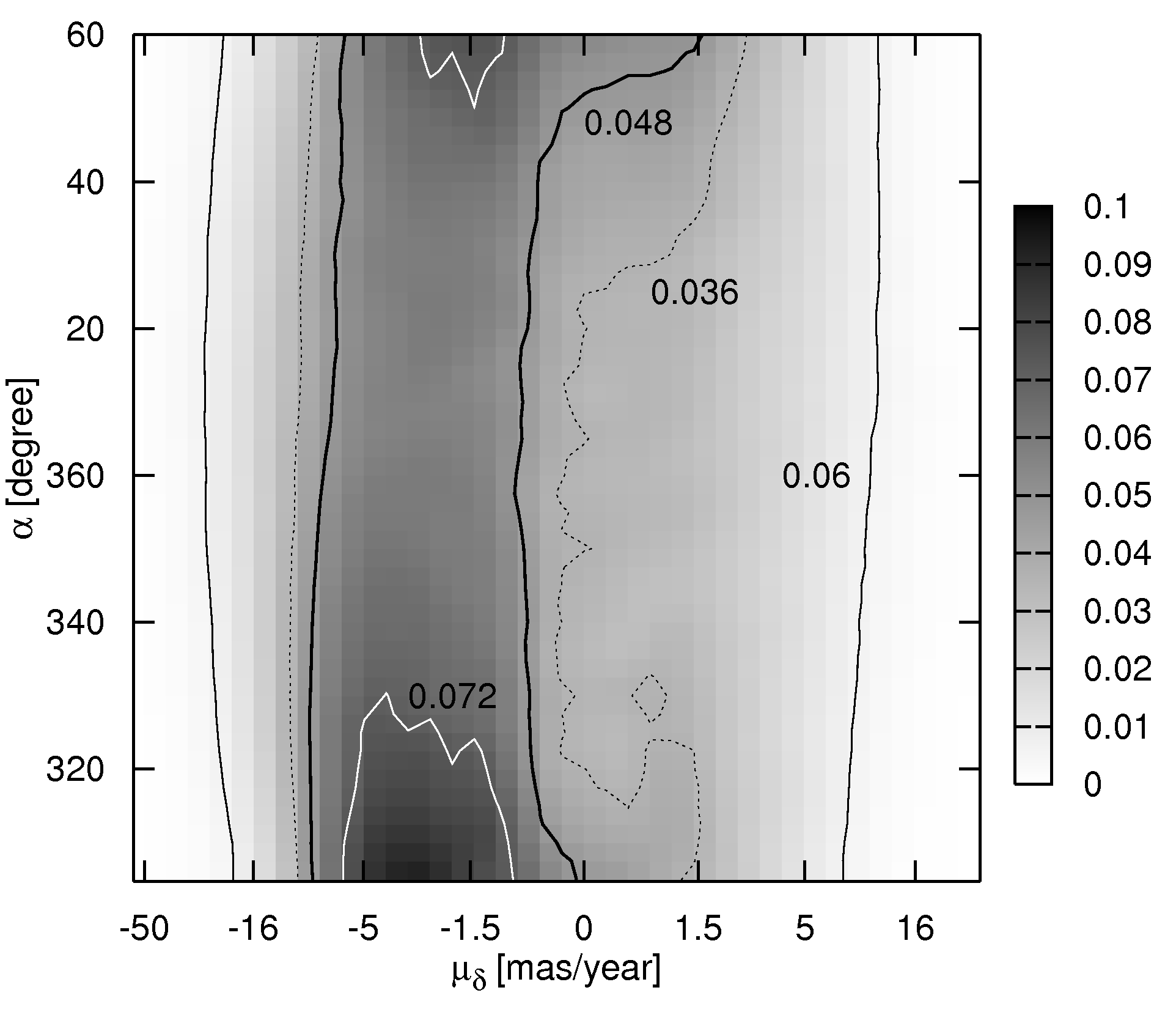
Figure 1.— Illustration of the first term of the prior (10) in the footprint of SDSS Stripe 82. The $\mu_{\delta}$ axis has an asinh() scale. As one moves into the direction of Galactic Plane (upwards and downwards on the figure), the probability distribution gets narrower since the velocity dispersion of stars decreases.

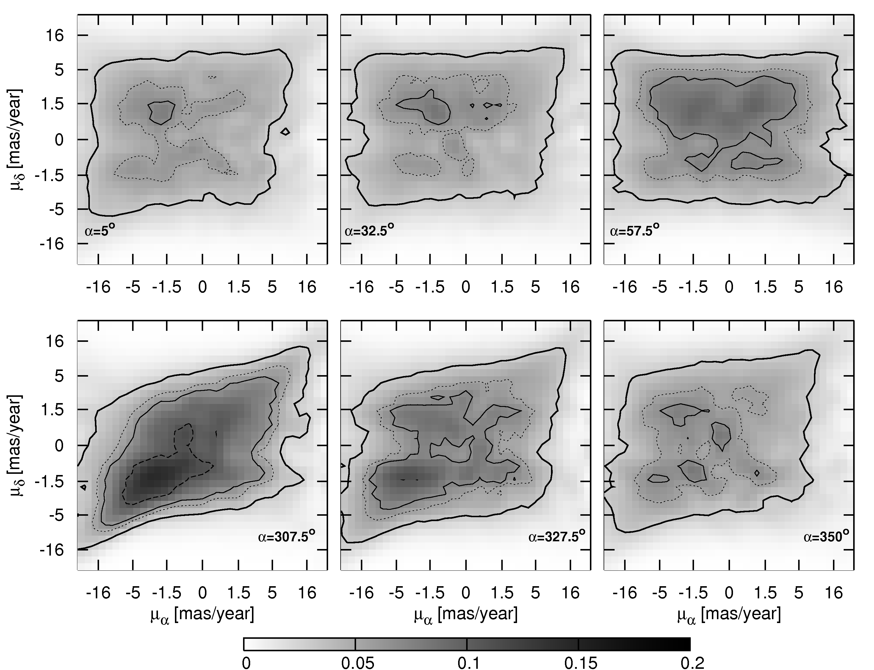
Figure 2.— Illustration of the second term of the prior (10). The function is 4-dimensional; The 6 different panels represent slices of the 4-dimensional PDF in the R.A. direction.

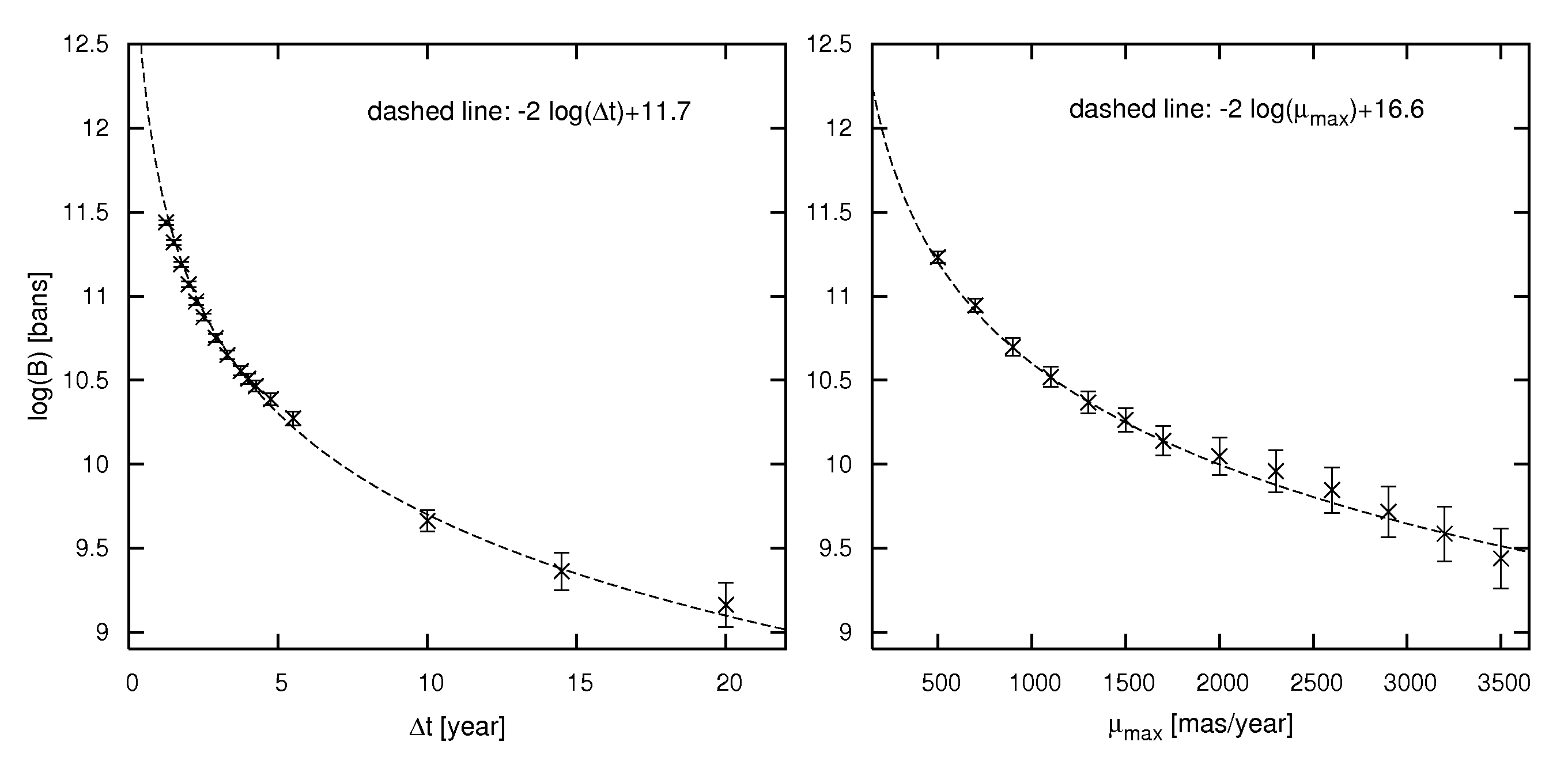
Figure 3.— Effects of time difference and proper motion limit on Bayes factor in case of uniform prior. In the left panel, we consider a mock observation pair with 0.54” separation and vary time intervals. The right panel shows the Bayes factor of a 360 mas/yr star with $\Delta{}t=2$ years as a function of the proper motion limit; see Equation (9). The error bars represent the uncertainty of numerical integration.

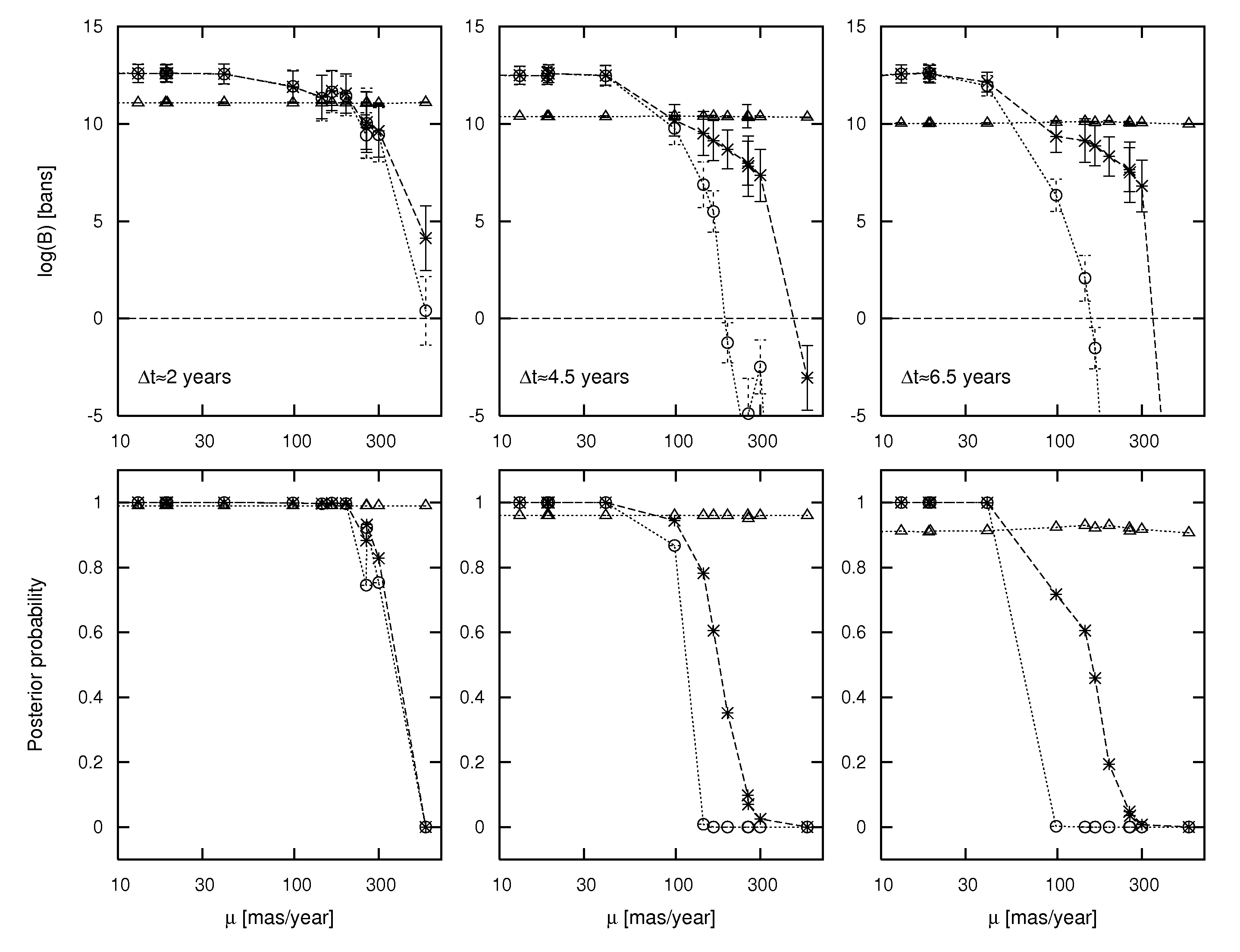
Figure 4.— Illustration of the weight of evidence (upper panels) and posterior probability (lower panels) as a function of proper motion in case of 2 observations with variable time differences (increasing from the left to the right). The proper motion is shown on a logarithmic scale. Open circles represent the static model, the triangles and crosses correspond to the values from the constant proper motion and the empirical prior, respectively. These values are also presented in Table 1.

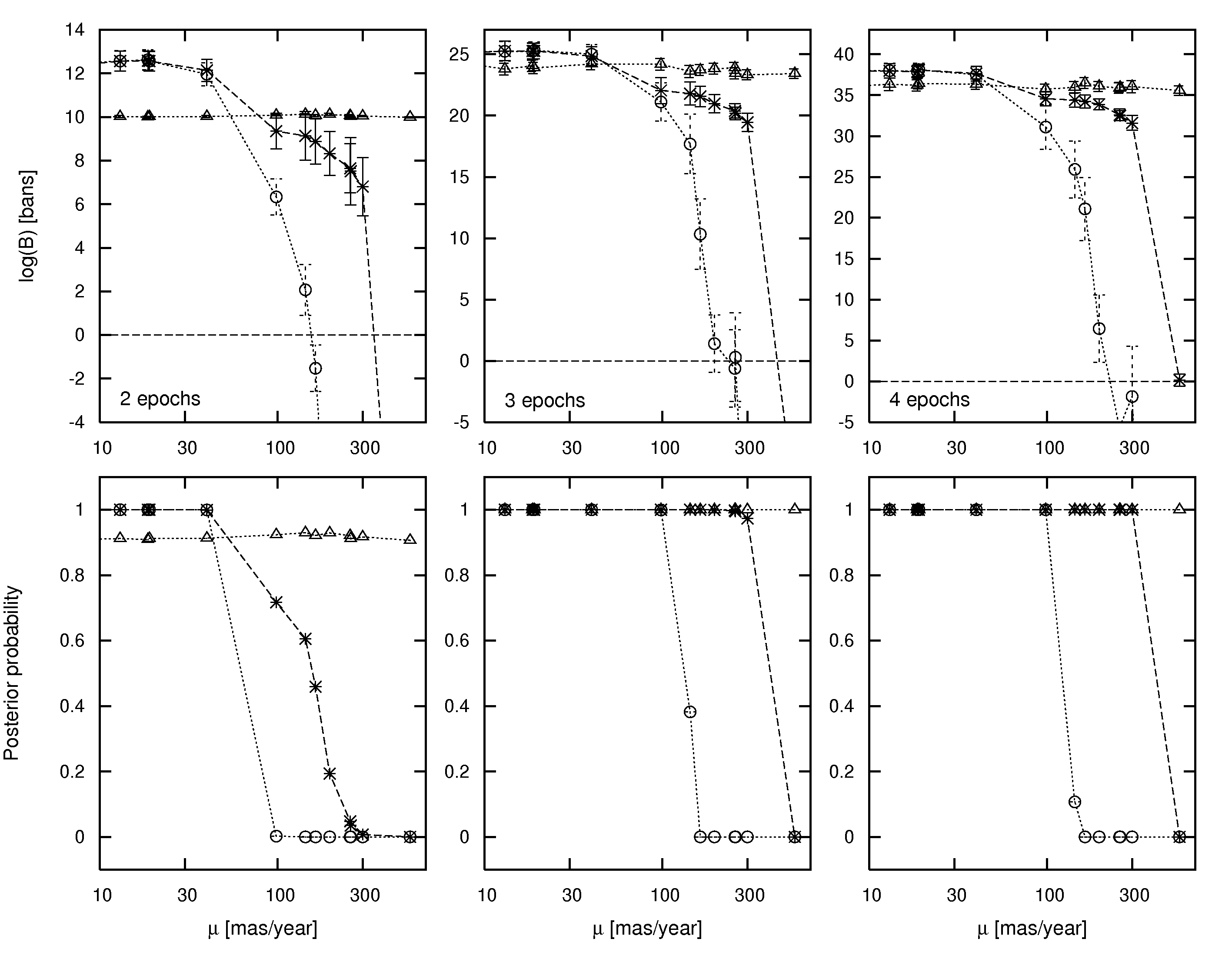
Figure 5.— The Bayes factor and posterior probability as a function of the proper motion in case of 2-, 3- and 4-way associations, increasing from left to right, see text. These values are also presented in Table 2.

.

3.1. Ensemble Statistics

To derive a more realistic $p(\mbox{\boldmath{$\mu$}}|\mbox{\boldmath{$r$}},H)$ prior, we choose to study the ensemble statistics of stars instead of approaching the problem with an analytic model. While the latter would have the advantage of providing a function at an arbitrary resolution, the formulas are difficult to derive and the analytic approximations might miss subtle details of the relation that could be relevant.

We study the properties of stars in the Sloan Digital Sky Survey catalog archive that also contains accurate proper motion measurements from the recalibrated United States Naval Observatory B1.0 Catalog (USNO-B; Munn et al., 2004). For this analysis, we pick stars from the Stripe 82 data set where multiple observations are available over 300 square degrees strip covering a narrow range in declination between $\pm 1.25^{\circ}$. These repeated observations were taken between June and December each year from 1998 to 2005 (Adelman-McCarthy et al., 2008). After rejecting saturated and faint sources (u should be in the range of 15–23.5 and g, r, i, z in the range of 14.5–24), the number of stars is around 100,000. This size does not allow for a high-resolution determination of the prior, hence we analyze additional simulation data.

To extend the number of stars used in constructing the prior, we used the current state-of-the-art Besançon models (Robin et al., 2003) that match the SDSS distributions well. Assuming four different stellar populations in the Milky Way, using the Poisson equation and collisionless Boltzmann equation with a set of observational parameters (i.e. fitting parameters to the dynamical rotation curve), they compute the number of stars of a given age, type, effective temperature and absolute magnitude, at any place in the Galaxy. The model has been successfully used for predictions of kinematics and comparison with observational data in studies, e.g., (Bienaymé et al., 1992), (Chareton et al., 1993), (Ojha et al., 1999), (Rapaport et al., 2001), (Soubiran et al., 2003). A total of $740,000$ stars were generated from the Besançon models using large-field equatorial coordinates, thus the prior is dominated by model data and not by SDSS measurements. The proper motion distribution of SDSS data and that of the model are very consistent, with the model yielding somewhat wider distributions than the observations.

In preparation for binning the data, we separate the dependence of the prior on the different proper motion components, $\mbox{\boldmath{$\mu$}}=(\mu_{\alpha},\mu_{\delta})$, and, omitting the explicit hypothesis, we write

$$p(\mu_{\alpha},\mu_{\delta}|\mbox{\boldmath{$r$}})=p(\mu_{\delta}|\mbox{\boldmath{$r$}})\,p(\mu_{\alpha}|\mu_{\delta},\mbox{\boldmath{$r$}})$$ (10)

Since the Stripe 82 data set in SDSS contains sources only in a narrow declination range between $-1.26^{\circ}$ and $+1.26^{\circ}$, we can safely neglect the dependence on declination in Equation (10) for the purpose of this study, thus

$$p(\mu_{\alpha},\mu_{\delta}|\mbox{\boldmath{$r$}})\approx p(\mu_{\delta}|\alpha)\,p(\mu_{\alpha}|\mu_{\delta},\alpha)$$ (11)

We establish these relations one-by-one starting with the former using the basic property of conditional densities

$$p(\mu_{\delta}|\alpha)=\frac{p(\mu_{\delta},\alpha)}{\int\!p(\mu_{\delta}^{\prime},\alpha)\,d\mu_{\delta}^{\prime}}$$ (12)

To achieve a better signal-to-noise behaviour across the entire parameter space, we do not use a uniform grid but vary bin sizes so that they follow the asinh() in both parameters. In this way one can have higher resolution bins where more data are available (around the peak close to 0) and wider bins in the tail. We further improve the quality of the empirical prior by removing high-frequency noise with a convolution filter, whose characteristic width is approximately one pixel in size at any location. The integral in the denominator is evaluated by counting the stars in the appropriate bins using the widths of the bins to weight the counts.

Figure 1 shows the prior using the aforementioned non-linear scale for $\mu_{\delta}$ as function of the position $\alpha$. The distribution is centered on approximately $-3\,\rm{mas}/\rm{yr}$, and the location of the mode is practically independent of the R.A. As one nears to the direction of the Galactic Plane ($\alpha=60^{\circ}$ and $\alpha=305^{\circ}$ are the nearest regions in this stripe) the distribution becomes sharper. This is to be expected as, if we included a broader range in Right Ascension, the PDF would get even narrower as the velocity dispersion of stars decreases.

The second term of Equation (11) is constructed similarly using the same adaptive binning and smoothing but in even higher dimensions. It is difficult to visualize a 4-dimensional PDF, hence, in Figure 2, we plot slices of the prior at various $\alpha$ values. Both axes are shown in the transformed scale. The values $\alpha=57.5^{\circ}$ and $\alpha=307.5^{\circ}$ represent the two edges of Stripe 82, which are closest parts to the Galactic Plane. The same effect can be seen on these panels as on Figure 1, looking out of the Plane the PDF gets more disperse. The boxy (squared) shape of the contour lines arises from the asinh() transformation; on a linear system, the contours would appear to be more circular.

4. Discussion

4.1. Sample Stars

As mentioned earlier, Stripe 82 was observed repeatedly from 1998 to 2005, between June and December of each year. Thus we can obtain multi-epoch observations to test our method. We choose a range of stars with different proper motions observed at different epochs. To be sure that for our tests the observed stars are the same in each epoch we select bright stars (magnitude $r<17$) with tolerances in all magnitudes (typically 0.7 in u, 0.4 in g, r, i and 0.5 in z). The query gives us on the average 20 epochs per star, from which many were observed with small time intervals while the biggest time interval between the epochs is approximately 6.5 years. We divide the time interval into 3 approximately equal parts and thus get 4 observations of each star with much the same time intervals between them. According to Equations (5) and (6), only RA and Dec coordinates are used for calculating the Bayes factors, USNO measurements of proper motion on the forthcoming figures and tables are only shown as a reference. We randomly select a dozen stars for the following tests.

4.2. Numerical Integration

We calculate the integrals of the Bayes factor numerically. Our Monte-Carlo implementation generates independent random positions $\{\mbox{\boldmath{$r$}}_{n}\}$ (3-D unit vectors) and two random components of the velocity that yield the $\mbox{\boldmath{$\mu$}}_{n}$ vector in the tangent plane of each $\mbox{\boldmath{$r$}}_{n}$, i.e.,

$$\mbox{\boldmath{$r$}}_{n}^{\prime}=\left(\mbox{\boldmath{$r$}}_{n}+\mbox{\boldmath{$\mu$}}_{n}\,\Delta{}t\right)\Big{/}\left|\mbox{\boldmath{$r$}}_{n}+\mbox{\boldmath{$\mu$}}_{n}\,\Delta{}t\right|$$ (13)

In theory, one has to integrate the position over the whole celestial sphere, and the proper motion out to infinity, but the integrands always drop sharply in practice, hence one can bound all the relevant parameters easily to reduce the computational need and to use the above approximation to the motion. For more efficient implementations, one can utilize more sophisticated Markov chain Monte Carlo (MCMC) methods.

The uncertainty estimates include two separate sources of errors. The numerical imprecision is tuned by the number of generated random parameters, and can be estimated in the process of the integration. In our calculations, this error term is kept at a low level, and contributes $10^{-2}$ order of magnitude to the value of the weight of evidence.

Another source of error comes from the uncertainty in position measurements. While this is small for the SDSS detections, $\sigma=0.1"$, the short time differences could yield large relative errors in the proper motion. To get the order of this error, we generate 100 random realizations of the position of every star from the appropriate Gaussian distribution, and recalculate the Bayes factor to derive the root-mean-square error in the weight of evidence. The figures later in this section contain error bars that represent these 1$\sigma$ deviations.

4.3. The Uniform Proper Motion Prior

After the static case, the simplest is a uniform prior as introduced in Equation (9). This analytic formula may appear at first not to favor any particular proper motion, yet the Bayes factor has some non-trivial scaling properties that are worth considering.

As the displacement of the source is a product of the time difference and the proper motion, associations at the same distances but with varying time intervals will indeed have different Bayes factors. In the case of a longer $\Delta{}t$, only smaller proper motions will contribute to the integral in Equation (5) shrinking the integral domain. This yields a scaling by a factor of $\Delta t^{-2}$, as seen in the left panel of Figure 3. This means that associations will be assigned lower qualities if they are farther in time even if their angular separations are identical.

Another interesting aspect is the selection of the limiting $\mu_{\rm{max}}$ value. Our choice of 600 mas/yr is admittedly somewhat arbitrary and was selected to cover the stars in our sample. If one decreased its value then stars moving at faster speeds would quickly get lower Bayes factors and clearly not be associated. Increasing limits make the value of the constant prior drop, which in turn will lower the quality of the associations. For illustrating this effect we compute the Bayes factors for a star with $\mu=360\ \rm{mas}/\rm{yr}$ and $\Delta{}t=2$ years as a function of $\mu_{\rm{max}}$, see the right panel of Figure 3. As the prior is proportional to $\mu_{\rm{max}}^{-2}$, the curve follows the same trend.

4.4. The Time Difference

First we analyze the quality of the associations as a function time difference between the observations. The top panels of Figure 4 show the logarithm of the Bayes factor, a.k.a. the weight of evidence for all stars in our test sample as a function of their proper motion. Open circles represent the results from the static model that can be obtained analytically as in Budavári & Szalay (2008), and crosses show the new measurements from the numerical integration of the improved model using the empirical prior introduced in this study. Triangles signal the value for a simple model of constant proper motion prior with $\mu_{\rm{max}}=600\ \rm{mas/yr}$. If we correct for small relative differences in time intervals between the epochs taking 2, 4.5 and 6.5 years as a reference respectively, this prior yields practically constant weights of evidence. For reference, the $W=0$ threshold is plotted as the dashed horizontal line. This is the theoretical dividing line above which the observations support the hypothesis of the match. All panels contain the same objects but the calculations are based on different detections that are farther apart in time as we go from left to right. What we see immediately is that as the time difference increases, the models provide increasingly different results: the static model starts rejecting stars with larger proper motions much faster than models that accommodates the possibility of the sources moving.

While the only objective measure of the quality for the match is the Bayes factor, its interpretation for the uninitiated is admittedly not as obvious at first as a probability value would be, where one has a good sense of the meaning of the values. From the Bayes factor, we can calculate the posterior $P(H|D)$, if we have a prior $P(H)$ via the equation

$$P(H|D)=\left[1+\frac{1-P(H)}{B(H,K|D)\,P(H)}\right]^{-1}$$ (14)

Assuming a constant prior over the sky with the value of $P(H)=1/N$, where $N=10^{9}$ is the estimated total number of stars on the sky as computed from the average density in SDSS, we can plot the matching probabilities for comparison. Note that large posterior probabilities are not sensitive to small modulations in the density; it changes linearly only for small values of the Bayes factor. The bottom panels of Figure 4 use the same symbols as the top ones to illustrate the derived posteriors using the above constant prior. The difference between the models is possibly even more striking here: While the left panel has very similar estimates from the different models, with time the separations grow large enough to quickly zero out the probabilities for stars with proper motions larger than 100 mas/yr, whereas the new models keep the probabilities significantly larger. Table 1 contains the measurements for all stars as function of the time difference. The first column of the table is the identifier of the star, the ObjID in SDSS Data Release 6. The reference proper motion values are taken from ProperMotions table of the SDSS Catalog Science Archive, which combine the SDSS and the recalibrated USNO-B astrometry for a precise and reliable determination.

We see two important features of the associations using the new proper motion priors. The constant prior yields lower and lower Bayes factors as the elapsed time increases and the probability drops regardless of the proper motion. Even when the separations are small enough for the static model to perfectly recover the object, the constant proper motion prior yields a lower 90% probability. The empirical prior always outperforms the static model but, in this 2-epoch observation case, the probabilities of the fast stars fall below the constant case or any reasonable probability threshold.

4.5. Three and Four Epochs

Next we turn our attention to the potential improvements from including additional epochs to the data sets. For this comparison, we keep the first and last observations in time, hence the baseline is the same for all cases. We add to these two observations additional measurements whose epochs are between them in time. These 2-, 3- and 4-way associations are shown in the left, middle and right panels of Figure 5, respectively. It is apparent that adding new detections significantly improves the the proper motion models: the reasonably good associations of only two detections are promoted to essentially certain matches by including intermediate detections. In contrast, the static model continues to reject the associations of all high proper motion stars. We see that one of the stars with $\mu\sim{}100\ \rm{mas/yr}$ actually gets a high probability even in the static model, when the angular separation for only a few years between the epochs is small enough to recover the star.

Table 2 shows the measurements as a function of the number of epochs used in the calculations. We see that the empirical prior of the improved model assigns 100% probability of all stars when considering all 4 epochs, and even the 3-epoch computations would yield close to that with the $\mu=300\ \rm{mas/yr}$ star getting a lower 97%. The exception from this is the fastest star at $\mu=555\ \rm{mas/yr}$ in case of the empirical prior, whose probability is essentially 0 in all panels. The reason for this is that this star is one of the highest proper motion stars in Stripe 82 and even with the generated model stars, which appear in the prior, we have very few (roughly 40) high proper motion stars.

It is worth re-iterating the reason for and the consequence of these results. Associations of more than two detections benefit dramatically more from the proper motion prior because two points can always be connected with a straight line unlike three or more. In other words, the prior probability of two detections being on a great circle is 100% but for three or more it is small, hence such combinations will get boosted by the alignment. Having seen the convincingly large probabilities for the 3-way cases and assuming the same maximum time difference between observations, one can conclude that, for the time intervals we consider here, surveying strategies with 3 epochs are superior to those with only 2, but adding more would not improve noticeably our ability to correctly cross-identify the detections.

5. Conclusions

We presented an improved model for probabilistic cross-identification of stars, which accommodates the possibility of moving objects via a proper motion prior. Using the Bayesian approach of Budavári & Szalay (2008), we performed hypothesis testing with the new models on a sample of SDSS DR6 stars with known proper motions and compared the results to the static case. In accord with our expectations, we found that moving stars would be missed by association algorithms that neglect to model the motion, but using an empirical prior of the proper motion would assign larger observational evidence to the match and higher probabilities. The dependence of the quality of these cross-identifications was studied as a function of separation in time (and space) as well as using multi-epoch observations. The SDSS Stripe 82 sample provided a good test set with 2–4 detections at different times with a few years in between. The tests were done assuming a maximum proper motion of 600 mas/yr. We found that, even though the 2-epoch data sets benefit significantly from the proper motion model, the 3-epoch observations essentially recover the right associations even for fast-moving stars, and the 4-epoch cases yield 100% probabilities. We also conclude, that the empirical prior surpasses the static model for the whole range of proper motions, while the uniform prior performs better only for the high proper-motion stars.

Since the analytically computable static case is still a good model for most celestial sources, it is best to carry out the cross-identification in multiple steps: first finding associations using the static model, and then applying the more computer-intensive proper motion variant only to the remainder of sources. While it might be tempting to simply increase the positional errors to discover the associations of moving sources, the procedure would be far from optimal. The overall dominant effect of such changes is that the Bayes factor would drop slower with separation, and, since the angular distance is essentially divided by the uncertainty, a ten times larger $\sigma$ would practically yield associations out to ten times larger distances; most of them incidental. The improvement of our novel approach over such naive workarounds comes from using the true uncertainties and the high sensitivity of the algorithm to sources moving on a great circle as allowed by the proper motion model.

Table 1Weights of evidence and posterior probabilities in the static, uniform prior and the proper-motion models as a function the elapsed time between two observations

ObjID	$\mu$	$\Delta t$	Weight			Probability
	[mas/yr]	[yr]	static	uniform	motion	static	uniform	motion
587731173305614418	13	1.38	12.59	11.08	12.59	1.00	0.99	1.00
		3.20	12.47	10.37	12.49	1.00	0.96	1.00
		4.46	12.56	10.01	12.56	1.00	0.91	1.00
587730847429427304	18.6	2.01	12.59	11.08	12.59	1.00	0.99	1.00
		3.95	12.48	10.37	12.47	1.00	0.96	1.00
		5.16	12.63	10.00	12.58	1.00	0.91	1.00
587731173305876571	19	1.38	12.60	11.08	12.60	1.00	0.99	1.00
		3.20	12.58	10.37	12.58	1.00	0.96	1.00
		4.46	12.56	10.01	12.56	1.00	0.91	1.00
587731186187763779	40	2.01	12.55	11.09	12.56	1.00	0.99	1.00
		4.03	12.46	10.36	12.49	1.00	0.96	1.00
		6.13	11.95	10.02	12.14	1.00	0.91	1.00
588015509268725910	98	2.02	11.93	11.08	11.90	1.00	0.99	1.00
		5.15	9.76	10.41	10.18	0.87	0.96	0.94
		7.98	6.33	10.08	9.35	0.00	0.92	0.72
588015509271805995	143	2.02	11.32	11.08	11.38	1.00	0.99	1.00
		5.07	6.88	10.38	9.50	0.01	0.96	0.78
		7.18	2.07	10.12	9.13	0.00	0.93	0.61
588015509286813878	163	2.17	11.64	11.10	11.70	1.00	0.99	1.00
		5.01	5.50	10.38	9.13	0.00	0.96	0.61
		7.18	-1.52	10.07	8.88	0.00	0.92	0.46
588015509268201645	196	2.02	11.44	11.07	11.56	1.00	0.99	1.00
		6.11	-1.24	10.36	8.68	0.00	0.96	0.35
		7.98	-11.97	10.12	8.33	0.00	0.93	0.19
588015509273378938	255	2.04	9.41	11.05	9.82	0.75	0.99	0.88
		5.08	-7.07	10.39	7.98	0.00	0.96	0.10
		7.20	-24.16	10.06	7.65	0.00	0.92	0.05
588015509279342731	257	2.02	10.02	11.08	10.08	0.92	0.99	0.93
		5.17	-4.89	10.32	7.82	0.00	0.95	0.07
		7.18	-24.11	10.01	7.51	0.00	0.91	0.04
587730847426740272	300	1.94	9.43	11.04	9.63	0.75	0.99	0.83
		4.01	-2.49	10.37	7.35	0.00	0.96	0.02
		6.13	-22.84	10.04	6.81	0.00	0.91	0.01
588015509283930154	555	2.19	0.40	11.09	4.12	0.00	0.99	0.00
		4.11	-36.83	10.33	-3.05	0.00	0.96	0.00
		7.18	-139.78	9.99	-21.80	0.00	0.91	0.00

Table 2Weights of evidence and posterior probabilities in the static, uniform prior and proper-motion models for the 2-, 3- and 4-way associations

ObjID	$\mu$	$N_{\rm{obs}}$	Weight			Probability
	[mas/yr]		static	uniform	motion	static	uniform	motion
587731173305614418	13	2	12.56	10.01	12.56	1.00	0.91	1.00
		3	25.25	23.80	25.28	1.00	1.00	1.00
		4	37.99	36.33	37.98	1.00	1.00	1.00
587730847429427304	18.6	2	12.63	10.00	12.58	1.00	0.91	1.00
		3	25.24	24.06	25.27	1.00	1.00	1.00
		4	37.91	36.19	37.86	1.00	1.00	1.00
587731173305876571	19	2	12.56	10.01	12.56	1.00	0.91	1.00
		3	25.32	23.89	25.27	1.00	1.00	1.00
		4	38.11	36.41	38.08	1.00	1.00	1.00
587731186187763779	40	2	11.95	10.02	12.14	1.00	0.91	1.00
		3	25.01	24.21	24.84	1.00	1.00	1.00
		4	37.48	36.34	37.64	1.00	1.00	1.00
588015509268725910	98	2	6.33	10.08	9.35	0.00	0.92	0.72
		3	21.11	24.18	22.05	1.00	1.00	1.00
		4	31.10	35.74	34.56	1.00	1.00	1.00
588015509271805995	143	2	2.07	10.12	9.13	0.00	0.93	0.61
		3	17.69	23.60	21.79	0.38	1.00	1.00
		4	25.92	35.96	34.41	0.11	1.00	1.00
588015509286813878	163	2	-1.52	10.07	8.88	0.00	0.92	0.46
		3	10.33	23.71	21.56	0.00	1.00	1.00
		4	21.10	36.48	34.22	0.00	1.00	1.00
588015509268201645	196	2	-11.97	10.12	8.33	0.00	0.93	0.19
		3	1.41	23.82	20.97	0.00	1.00	1.00
		4	6.46	36.08	33.88	0.00	1.00	1.00
588015509273378938	255	2	-24.16	10.06	7.65	0.00	0.92	0.05
		3	-0.61	23.88	20.39	0.00	1.00	1.00
		4	-5.76	35.87	32.60	0.00	1.00	1.00
588015509279342731	257	2	-24.11	10.01	7.51	0.00	0.91	0.04
		3	0.30	23.44	20.18	0.00	1.00	0.99
		4	-5.44	35.95	32.49	0.00	1.00	1.00
587730847426740272	300	2	-22.84	10.04	6.81	0.00	0.92	0.01
		3	-21.3	23.32	19.46	0.00	1.00	0.97
		4	-1.85	36.05	31.60	0.00	1.00	1.00
588015509283930154	555	2	-139.78	9.99	-21.80	0.00	0.91	0.00
		3	-37.41	23.42	-11.46	0.00	1.00	0.00
		4	-129.09	35.56	0.17	0.00	1.00	0.00

References

- Adelman-McCarthy et al. (2008) Adelman-McCarthy, J.K. et al. 2008, ApJS, 175, 297-313
- Bienaymé et al. (1992) Bienaymé O., Mohan V., Crézé M., Considére S., Robin A. C., 1992, A&A, 253, 389
- Budavári & Szalay (2008) Budavári, T., & Szalay, A. S. 2008, ApJ, 679, 301
- Chareton et al. (1993) Chareton M., Considére S., Bienaymé O. 1993, A&AS, 102, 649
- Fisher (1953) Fisher, R., 1953, Proceedings of the Royal Society of London, Series A, Mathematical and Physical Sciences, Vol. 217, No. 1130., pp.295–305
- Munn et al. (2004) Munn et al. 2004, AJ, 127, 3034. ”An Improved Proper-Motion Catalog Combining USNO-B And The Sloan Digital Sky Survey”
- Ojha et al. (1999) Ojha, D. K., Bienaymé, O., Mohan, V., & Robin, A. C. 1999, A&A, 351, 945
- Rapaport et al. (2001) Rapaport, M., Le Campion, J.-F., Soubiran, C., Daigne, G., Pri, J.-P., Bosq, F., Colin, J., Desbats, J.-M., Ducourant, C., Mazurier, J.-M., Montignac, G., Ralite, N., Rquime, Y.,Viateau, B. 2001, A&A, 376,325
- Robin et al. (2003) Robin, A. C., Reylé, C., Derriere, S. & Picaud, S. 2003, A&A, 409, 523
- Soubiran et al. (2003) Soubiran, C., Bienaymé, O., Siebert, A. 2003, A&A, 398, 141
- York et al. (2000) York, D.G., et al. 2000, AJ, 120, 1579