Yukawa particles confined in a channel and subject to a periodic potential: ground state and normal modes

Abstract

We consider a classical system of two-dimensional (2D) charged particles, which interact through a repulsive Yukawa potential $exp(-r/\lambda)/r$, confined in a parabolic channel which limits the motion of the particles in the $y$-direction. Along the $x$-direction, the particles are also subject to a periodic potential substrate. The ground state configurations and the normal mode spectra of the system are obtained as function of the periodicity and strength of the periodic potential ($V_{0}$), and density. An interesting set of tunable ground state configurations are found, with first and second order structural transitions between them. A magic configuration with particles aligned in each minimum of the periodic potential is obtained for $V_{0}$ larger than some critical value which has a power law dependence on the density. The phonon spectrum of different configurations were also calculated. A localization of the modes into a small frequency interval is observed for a sufficient strength of the periodic potential. A tunable band-gap is found as a function of $V_{0}$. This model system can be viewed as a generalization of the Frenkel and Kontorova model.

I Introduction

Two-dimensional system (2D) are often created in the presence of a substrate Grnberg , which may induce a periodic potential on the particles. In the pioneering experimental work of Chowdhury $et$ $al.$ Chowdhury , the authors studied a 2D colloidal system under influence of an one-dimensional (1D) periodic potential. An optical tweezer was used to trap the colloids by laser beams. For very high values of light intensity, crystallization of the colloidal suspension was observed, when the periodicity of the substrate (periodic potential) was chosen to be commensurate to the mean particle distance. Laser induced freezing which is caused by the suppression of thermal fluctuations transverse to the 1D periodic substrate was found (liquid-solid transition) bechinger01 . The system studied in Ref. Chowdhury is related to the colloidal molecular crystal (CMC) and received attention recently due to important applications in photonic and phononic crystals reich1 ; reichhardt02 .

Specifically, CMC occurs when the number of colloids is an integer multiple of the number of substrate minima, and has been investigated using in simulations reichhardt02 ; mikulis04 and realized experimentally bechinger02 . CMC is an interesting experimental system to study order and dynamics in 2D since typical particle size and relaxation times permit, e.g, to use digital video-microscopy to track particle trajectories, allowing a deeper investigation of the physical behavior of the system alsayed05 .

Originally, CMC was proposed for 2D system in 2D periodic potential (substrate). As known the dimensionality of the system plays an important role in many physical properties of distinct physical phenomena. In this sense, an interesting question is how the ordered structures and physical properties would be influenced by the dimensionality of the periodic substrate. Recently, Herrera-Velarde and Priego herrera1 ; herrera2 studied a 2D system of repulsive colloidal particles confined in a narrow channel and subject to an external 1D periodic potential, which could be seen as the 1D version of the CMC. The main focus of the study was the role of the substrate in the mechanisms that lead to a variety of commensurate and non-commensurate phases, its effect on the the single-file diffusion regime, and the pinning-depinning transition in 1D systems. The 1D character of the channel was represented by a hard wall potential. Due to the repulsive interaction between the particles and the nature of the confinement potential the density across the channel was found to be non-uniform with a higher density at the channel edges.

In the present paper we study the ordered configurations and the phonon spectrum of a 2D system of repulsive (Yukawa interaction) particles confined in a parabolic channel and subjected to a 1D periodic potential along the channel. As compared to the systems in Refs. herrera1 ; herrera2 , and due to the parabolic shape of the confinement an opposite density distribution is observed, with particles more concentrated at the central region of the channel. As shown previously for finite size clusters of repulsive particles, the confinement potential is determinant, e.g. for melting and phonon spectra bedanov94 . The 1D parabolic confinement introduces a $quasi$-1D (Q1D) character to the system in the sense that particles are still allowed to move freely in the perpendicular direction of the confinement potential.

The interplay between the repulsive inter-particle interaction and the periodic potential determines the different ground state configurations. Our model system of Yukawa particles can be realized experimentally using: i) a dusty plasma chu1994 ; liu03 ; liu05 , ii) colloidal systems zahn99 ; golosovsky02 and iii) electrons on liquid helium wigner1 ; wigner2 . A dusty plasma consists of interacting microscopic dust particles immersed in an electron-ion plasma. The dust particles acquire a net charge and the Coulomb interaction between the dust-particles is shielded by the electron-ion plasma resulting in a Yukawa or screened Coulomb inter-particle interaction. The dust particles are confined to a two-dimensional layer through a combination of gravitational and electrical forces. By microstructuring a channel in the bottom electrode of the discharge it is possible to laterally confine the dust particles as was realized in Refs. 1homann ; 2misawa ; 3liu ; 4nelser ; 5sheridan , the strength of the 1D confinement potential can be varied by the width of the channel or the potential on the bottom electrode. When the width of the channel is microstructured into an oscillating function along the channel it will result in a periodic potential along the channel.

Alternatively, one can confine charged colloids, that move in a liquid environment containing counterions, into microchannels as e.g. recently realized experimentally in 6 . In this case the inter-colloid interaction can be modeled by a screened Coulomb interaction and the confinement potential is a hard wall potential. By changing the depth profile of the micro-channel it has been shown in 7 that the confinement potential can be tuned into a harmonic potential. Micro-structuring the width of the channel into an oscillating function along the channel will result into an additional periodic potential along the channel.

In a previous work gio04 the ordered configurations of Yukawa particles confined to Q1D were studied. A phase diagram was obtained as function of the particle density and inverse Debye screening length which is a measure of the strength of the inter-particle interaction. The competition between the lateral confinement and the screened Coulomb interaction resulted in different phases where the particles are ordered in chains. The most well studied phases are the one- and two-chain configurations where the transition between those two phases occurs through a zig-zag transition. The latter is a continuous transition as found theoretically for mono- gio10 and bi-disperse wpferreira ; wand10 systems, and experimentally 4nelser ; 5sheridan with a power law dependence on the width Candido ; gio10 . Here we are interested to investigate how the phase diagram will be modified when an additional 1D periodic potential is present. For example, how the zig-zag transition will be modified by the periodic potential.

The present paper is organized as follows. In Sec. II we describe the model system and methods used in the calculation of the properties. In Sec. III we present the results for the different ground state configurations. In Sec. IV the normal mode spectra for the one and two-chain regimes are presented for different intensities of the periodic potential. Our conclusions are given in Sec. V.

II THE MODEL

Our system consists of identical point-like particles interacting through a screened Coulomb potential. The particles are allowed to move in a two-dimensional (2D) plane and are subject to an external parabolic confinement in the y-direction and a periodic substrate potential along the $x$-direction. A sketch of the present model system is shown in Fig. 1. The total interaction energy of the system is given by

$${\rm{H^{\prime}=}}\frac{{{\rm{\textit{q}}}^{\rm{2}}}}{{\varepsilon}}\sum\limits_{i<j}{\frac{{e^{-|{\vec{r^{\prime}_{i}}-\vec{r^{\prime}_{j}}}|/\lambda}}}{{\left|{\vec{r^{\prime}_{i}}-\vec{r^{\prime}_{j}}}\right|}}}+\sum\limits_{i}{\frac{1}{2}}m\omega_{0}^{2}{y^{\prime}_{i}}^{2}+V_{0}^{\prime}\sum\limits_{i}{\cos(\frac{{2\pi x^{\prime}_{i}}}{L})}$$ (1)

where $\epsilon$ is the dielectric constant of the medium in which the particles are moving in, $\lambda$ is the Debye screening length, $V_{0}^{\prime}$ is the strength of the periodic substrate potential, $L$ is the periodicity of the substrate potential, and $\mathbf{r^{\prime}}_{i}=(x^{\prime}_{i},y^{\prime}_{i})$ is the position of the $i^{th}$ particle. In order to keep in Eq. (1) only the parameters which rule the physics of the system, it is convenient to write the energy and the distances in units of $E_{0}=(m\omega_{0}^{2}q^{4}/2\epsilon^{2})^{1/3}$ and $r_{0}=(2q^{2}/m\epsilon\omega_{0}^{2})^{1/3}$, respectively, and the screening parameter $\kappa=r_{0}/\lambda$, where. We also define the dimensionless strength of the substrate potential $V_{0}=V_{0}^{\prime}/E_{0}$ and $\vec{r}=\vec{r^{\prime}}/r_{0}$. In so doing, the expression for the energy is reduced to

$${\rm{H=}}\sum\limits_{i<j}{\frac{{e^{-\kappa|{\vec{r_{i}}-\vec{r_{j}}}|}}}{{\left|{\vec{r_{i}}-\vec{r_{j}}}\right|}}}+\sum\limits_{i}{y_{i}}^{2}+V_{0}\sum\limits_{i}{\cos(\frac{{2\pi x_{i}}}{L})}$$ (2)

As can be observed from Eq. (2) the system is a function of the parameters, $\kappa$, $V_{0}$, $L$, and the density. In our numerical calculations $\kappa=1$, which is a typical value for dusty plasma and colloidal systems. We introduce a distance $a_{0}$, which is defined as the distance between particles when $V_{0}=0$. The density (n) is the ratio between the number of chains $N_{ch}$ and $a_{0}$, i.e. $n=N_{ch}/a_{0}$. In this case, the system self-organizes in a multichain-like structure gio04 .

The model studied in this work is related to the Frenkel-Kontorova (FK) model, which is a simple one-dimensional model that describes the dynamics of a chain of particles interacting with nearest neighbors in the presence of an external periodic potential. This model was initially introduced in the 1930s by Frenkel and Kontorova and was subsequently reinvented independently by others, notably Frank and Van der Merwe pcm . It provides a simple and realistic description of commensurate-incommensurate transitions when thermal fluctuations are unimportant.

In the present work the quasi-1D character of our system makes it different from the 1D FK-model. The particles have the additional freedom to move perpendicular to the chain which leads to a rich set of new phases. The presence of two length scales in the FK-model, i.e. the inter-particle distance and the periodicity of the 1D potential, is the reason of the complex behavior of the model. The inter-particle potential favors a uniform separation between the particles, whereas the V(x) tends to pin the particles at the minima of the periodic potential. This competition between both interactions is often called frustration or length scales competition.

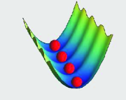
Figure 1: (Color online) A sketch of the model system.

The minimum energy configurations are obtained by numerical and analytical calculations. In the numerical simulations, we typically considered 100-200 particles, together with periodic boundary conditions in the unconfined direction in order to mimic an infinite system. We do not consider friction in the present paper. In spite of the primary importance of friction to the motion of the particles in real systems, the ground state configurations are not affected by it.

Notice that the substrate is defined in terms of the parameter $L$. Comparing $L$ and $a_{0}$, we define here an initially commensurate (IC) when ($L/a_{0}=p/q$, with $p$ and $q$ integers) and initially non-commensurate (INC) regime of the ordered structures when the ratio $L/a_{0}$ is a irrational number. It should be emphasized that in these cases the inter-particle distance $a_{0}$ is defined in the absence of a substrate ($V_{0}=0$). In the case $V_{0}\neq 0$, it is expected that the mean distance between particles along a given chain $a$ changes as a function of $V_{0}$, driving the system to new commensurate or non-commensurate configurations.

III Ground State Configurations

In this section, we present the results obtained analytically and numerically for the ground state configurations. In the former, we calculate the energy per particle for different configurations as a function of the strength and periodicity of the substrate. We minimize such expressions with respect to the different distances between particles. The configuration with lowest energy is the ground state. In order to predict which structures should be taken into account in the analytical approach, we also use molecular dynamic simulations as a complementary tool. The numerical method can give us some hints about which structures to consider. It should be noticed that one of the draw backs of the numerical technique is that in some cases there exist a larger number of meta-stable states, mainly in the limit of high densities where the system is found in a multi-chain structure. On the other hand, the numerical approach is the only way to obtain the ground state configurations in some incommensurate regimes, which will be analyzed in the next sections.

We show here that depending on the periodicity of the substrate we can tune the ground state configuration, induce structural phase transitions and control the number of chains. This is interesting from an experimental point of view, since the number of chains can be associated with the porosity of the system, making it a controllable filter.

The main features of the present model system can be already seen in the more simple situations of the single- and two-chain regimes. For this reason, we limit ourselves to these cases, because it simplifies the physical interpretation of our results.

III.1 Single-chain regime

As an example, we study in this section systems with densities $n=0.5$ and $n=0.7$, which are found in the single-chain regime gio04 in the absence of the substrate $V_{0}=0$. For $n=0.5$ we consider the commensurate ratios $L/a_{0}=1$ and $L/a_{0}=2$, while for $n=\sqrt{2}/{2}$ we consider the non-commensurate regime with $L/a_{0}=\sqrt{2}$.

The simplest IC configuration is the trivial single-chain regime where each particle is sitted in a minimum of the periodic potential with $n=0.5$ and $L/a_{0}=1$. In this case, the configuration remains the same for any value of $V_{0}$. Notice that the cases in which $L/a_{0}=1/I$, where $I\geq 1$ is an integer, will exhibit the same behavior, since each particle is positioned exactly in a minimum of the substrate potential. On the other hand, the case $L/a_{0}=I$ is very different and the particle configuration depends strongly on $V_{0}$, as will be shown in the next paragraph.

In the IC case with $n=0.5$ and $L/a_{0}=2$, for small values of $V_{0}$ the particles are alternately located at the minimum and at the maximum of the substrate potential [see inset (a) in Fig. 2]. A sufficient increase of $V_{0}$ forces the system to a new single-chain configuration in which a pair of particles is located at each minimum of the substrate [see inset (b) in Fig. 2]. A further increase of $V_{0}$ pushes each pair of particles closer to each other, increasing the repulsive energy between them.

For a critical value of $V_{0}$ ($\approx 0.8$) a structural transition to the two-chain configuration is induced [see inset (c) of Fig. 2]. The system changes from a one to two-chains configuration. In the two-chain configuration the separation $d_{x}$ between particles in the x-direction of each minimum of the substrate is zero, which means particles are aligned along the y-direction. The separation $d_{y}$ between chains does not change as function of $V_{0}$. In this particular configuration $d_{y}$ is ruled only by the competition between the repulsive interaction between particles and the parabolic confinement, being independent of the strength of the periodic potential. The type of transition observed here is different from the one found in Ref. gio10 , where the authors demonstrated that in the absence of a periodic potential and in the presence of a parabolic confinement we have only continuous transitions from one to two chains. In our case the one- to two-chains transition is clearly a first-order phase transition as function of $V_{0}$. Notice that in the two-chain regime the system is re-organized in a final commensurate structure with a new ratio $L/a=1$. We can define here a commensurate-commensurate transition between different orders of commensurability.

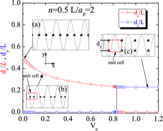
Figure 2: (Color online) Nearest neighbor separation between particles in the $x$- ($d_{x}$) and $y$-direction ($d_{y}$) as a function of $V_{0}$ for the case $n=0.5$ and $L/a_{0}=2$. Three possible configurations are shown as insets.

The expression for the energy per particle which is able to describe all phases observed in the case with $n=0.5$ and $L/a_{0}=2$ and in the case $n=1.0$ and $L/a_{0}=1$ is given by

$$\begin{split}E=&\frac{n}{2}\sum_{j}\frac{e^{-2\kappa j/n}}{j}+\frac{n}{4}\sum_{j}\frac{e^{-\frac{2\kappa}{n}\sqrt{[(j-1)+c_{x}]^{2}+c_{y}^{2}}}}{\sqrt{[(j-1)+c_{x}]^{2}+c_{y}^{2}}}\\ &+\frac{n}{4}\sum_{j}\frac{e^{-\frac{2\kappa}{n}\sqrt{(j-c_{x})^{2}+c_{y}^{2}}}}{\sqrt{(j-c_{x})^{2}+c_{y}^{2}}}+4\Big{(}\frac{c_{y}}{n}\Big{)}^{2}-\cos(\pi c_{x})\end{split}$$ (3)

where $c_{x}=d_{x}/L$ and $c_{y}=d_{y}/L$ are, respectively, the dimensionless separations between particles within a minimum of the periodic potential along the chain and perpendicular to it.

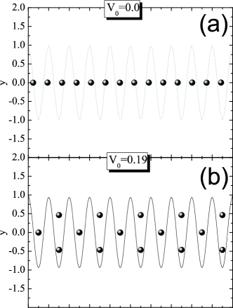
Figure 3: Ground state configurations for the case $n=\sqrt{2}$ and $L/a_{0}=\sqrt{2}$ for: (a) $V_{0}=0.17$ (b) $V_{0}=0.19.$

Now we discuss the INC regime with $n=\sqrt{2}$ and $L/a_{0}=\sqrt{2}$. The same general behavior of previous cases can be observed here, with several structural transitions ruled by the strength of the periodic substrate $V_{0}$ (Fig. 3). For a large enough $V_{0}$ the system can be found in a final commensurate regime with $L/a\approx 1/2$, but now in the three-chain configuration with particles almost uniformly distributed over chains.

III.2 Two-chain regime

In this section we consider the system with $n=1.0$, where a two-chain configuration is found as the ground state for $V_{0}=0$. Differently from what was observed in the one-chain configuration ($n=0.5$), when $L/a_{0}=1.0$, the two chain configuration remains, but the internal structure depends on $V_{0}$. This is shown in Fig. 4(a), where the relevant internal distances [Fig. 4(b)] for the arrangement are presented as function of $V_{0}$.

For $V_{0}=0.16$ the system changes from a staggered ($d_{x}\neq 0$) to an aligned ($d_{x}=0$) two-chain configuration, through a second order (continuous) structural transition, characterized by a discontinuity in the second derivative of the energy with respect to $V_{0}$. Notice that in the case $L/a_{0}=1.0$, there are always two particles per period of the substrate potential, and in such a commensurate phase the system is always found in the two-chain regime.

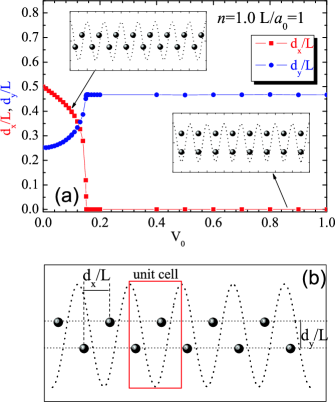
Figure 4: (Color online) (a) Inter-particle separation as function of $V_{0}$ for $n=1.0$ and $L/a_{0}=1.0$. (b) A sketch of the two-chain configuration with the distances $d_{x}$ and $d_{y}$ indicated.

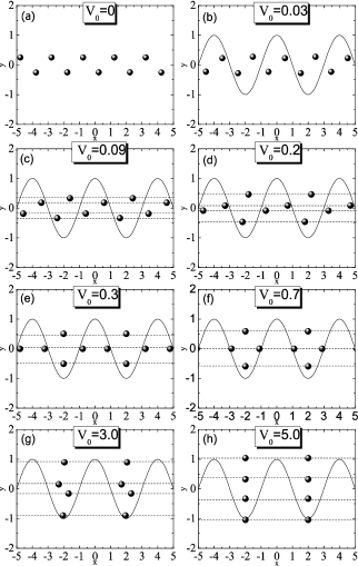
Figure 5: Ground state configurations for the case $n=1.0$ and $L/a_{0}=2$ for different values of $V_{0}$.

Next, we consider the more interesting case with $n=1.0$ and $L/a_{0}=2$. When $V_{0}$ is increased some unusual configurations appear as shown in Fig. 5. Initially the particles move in the x-direction towards the minima of the periodic potential and at the same time each chain starts to break up into two chains [Figs. 5(c)]. The transition found here is second-order.

With further increase of $V_{0}$ the two inner chains move towards each other [see Fig. 5(d)] and merge into a single chain in the center [see Figs. 5 (d,e,f)]. The particles in the outer chains move towards the minimum of the periodic potential [see Figs. 5 (d,e,f)]. With further increase of $V_{0}$ the pair of particles in the middle chain are pushed closer to each other and finally form a row of four particles directed along the y-direction and positioned in the minimum of the periodic potential [see Figs. 5 (g,h)]. The configurations presented in Fig. 5 indicates a tunable porosity of the system as function of $V_{0}$. This is very convenient feature if the system is settled to be used as a filter or sieve, as pointed out in Refs. dna1 ; dna2 , where superparamagnetic colloidal particles were self-assembled in chain-like structures and used for separation of DNA molecules.

The movement of the different particles in the x- and y-direction as function of $V_{0}$ is summarized in Fig. 6, where structural transitions are indicated by vertical dashed lines. Three second order structural transitions are observed as function of $V_{0}$ and the number of chains varies from $2\rightarrow 4\rightarrow 3\rightarrow 4\rightarrow 4$.

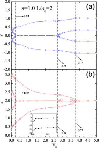
Figure 6: (Color Online) (a) The lateral $y$-position of chains for the case $n=1.0$ and $L/a_{0}=2$. The vertical dotted lines represents the values of $V_{0}$ where structural transitions occur. (b) The particle position in the $x$-direction as function of $V_{0}$.

Finally, we study the case with $n=1.5$ and $L/a_{0}=1.5$. Here the commensurate ratio changes according to $V_{0}$. Initially, for $V_{0}=0$, the system is arranged in two chains [see Fig. 7(a)], which are displaced with respect to each other over half the inter-particle distance in each chain. There are two particles per unit cell, which characterize an initially commensurate (IC) configuration.

When $V_{0}$ increases the system transits to a four-chain configuration through a second or first order structural transition, with the outer chains having twice as many particles as the inner chains [Fig. 7(b)]. Alternatively, we can also view this configuration as two chains of triangles as indicated in the shadowed region in Fig. 7(b). In this case $d_{2}>d_{3}$ and $d_{5}>d_{4}$ and the length of the unit cell is $d_{1}=d_{2}+d_{3}$. There are six particles in the unit cell, as in the case $V_{0}=0$.

With further increase of $V_{0}$, the y-distance $d_{6}$ between the internal chains goes to zero and the system changes to the three-chain configuration [Fig. 7(c)] with the same number of particles in each one, and the central chain shifted by $a/2$ along the x-direction with respect to the outer chains, which are aligned along the y-direction. Notice that in this case there are only three particles per unit cell. This is interesting since the number of normal modes is now half the one observed for the configuration presented in Fig. 7(b), where the number of particles in the unit cell is six. The reduction of the allowed excitation modes is controlled by the strength of the periodic potential, and this can be used as an important feature for possible application in phononics. For $V_{0}>0.5$, particles in different chains are all aligned along the y-direction and located in each minimum of the periodic substrate [Fig. 7(d)]. The trajectories of the different particles in the channel as function of $V_{0}$ is visualized in Fig. 8.

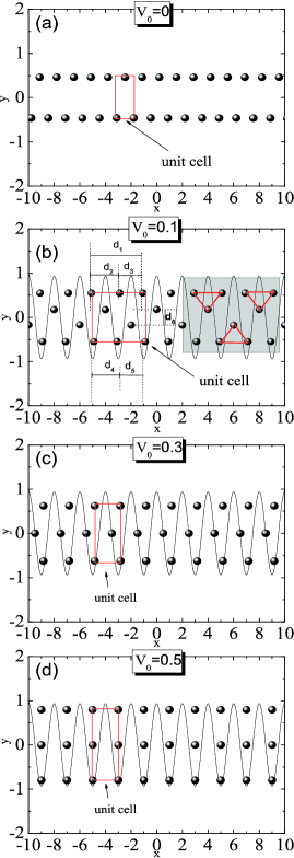
Figure 7: (Color online) Ground state configurations for different values of $V_{0}$ for $n=1.5$ and $L/a_{0}=1.5$. In (b) the relevant distances for the analytical calculation of the energy are presented.

Again, the relation between the periodicity of the substrate and the distance between particles is different from the case $V_{0}=0$, $L/a_{0}=1$. This is interesting since we can change the commensurability of the system by changing only the strength of the substrate potential.

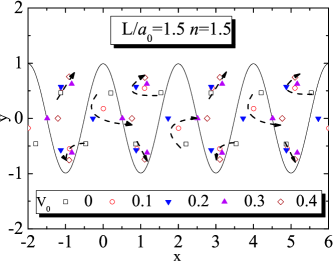
Figure 8: (Color Online) Particle trajectories for different values of $V_{0}$ near the potential minimum for the case $n=1.5$ and $L/a_{0}=1.5$.

As presented in Figs. 2(c), 4 and 5(h), for a critical value of $V_{0}$ the present model system is found in the special configuration where the particles are aligned along the confinement direction. Such a $y$-aligned configuration (YAC) occurs if the condition $L/a_{0}=p$, where $p$ is an integer ($\geq 1$), is satisfied. In this case, if N is the number of chains of the initial structure ($V_{0}=0$), then we find that the number of particles aligned along the $y$-direction in each minimum of the substrate potential is $N.p$, which is also the number of chains. The critical value of $V_{0}$ for which the YAC phase can be induced is obtained by adding the interaction between particles and confinement energies. A general expression for the YAC is given by:

$$\begin{split}V=&\frac{n}{{Np}}\sum\limits_{j}{\frac{{e^{-kNpj/n}}}{j}}\\ &+\frac{{2n}}{{N^{2}p^{2}}}\sum\limits_{q=1}^{Np-1}{\sum\limits_{l=q+1}^{Np}{\sum\limits_{j}{\frac{{e^{-kNp/n\sqrt{j^{2}+(p-q)^{2}c^{2}}}}}{{\sqrt{j^{2}+(p-q)^{2}c^{2}}}}}}}\\ &+\frac{n}{{N^{2}p^{2}}}\sum\limits_{q=1}^{Np-1}{\sum\limits_{l=q+1}^{Np}{\frac{{e^{-k(l-q)cNp/n}}}{{(l-q)c}}}}\\ &+\frac{{2c^{2}Np}}{{n^{2}}}\sum\limits_{l=1}^{Np/2}{(l-1/2)^{2},}\end{split}$$ (4)

in the case where $N.p$ is even, and

$$\begin{split}V=&\frac{n}{{Np}}\sum\limits_{j}{\frac{{e^{-kNpj/n}}}{j}}\\ &+\frac{{2n}}{{N^{2}p^{2}}}\sum\limits_{q=1}^{Np-1}{\sum\limits_{l=q+1}^{Np}{\sum\limits_{j}{\frac{{e^{-kNp/n\sqrt{j^{2}+(p-q)^{2}c^{2}}}}}{{\sqrt{j^{2}+(p-q)^{2}c^{2}}}}}}}\\ &+\frac{n}{{N^{2}p^{2}}}\sum\limits_{q=1}^{Np-1}{\sum\limits_{l=q+1}^{Np}{\frac{{e^{-k(l-q)cNp/n}}}{{(l-q)c}}}}\\ &+\frac{{2c^{2}Np}}{{n^{2}}}\sum\limits_{l=1}^{Np/2}{l^{2},}\end{split}$$ (5)

if $N.p$ is an odd number.

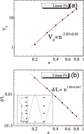
Figure 9: (Color online) (a) Critical value of $V_{0}$ as function of density for the YAC phase. (b) The distance between the particles along the y-direction as function of the density in the YAC phase. The inset shows a sketch of the general groundstate configuration with all relevant parameters. The red line in both figures is the linear fit.

The critical value of $V_{0}$ and the separation $d$ between particles in each minimum are presented in Fig. 9. A sketch of the configuration in each minimum of the periodic substrate with all relevant parameters is also shown as insect in Fig.9(b). A power law dependence of $V_{0}$ and $d/L$ on the density is found.

IV Phonon Spectrum

Next, we analyze the $V_{0}$-dependence of the normal mode spectrum. We follow the standard harmonic approximation and take into account the periodicity of the system in the unconfined direction ($x$-axis).

The present model system is a strictly 2D system where the number of particle in the unit cell and the number of degrees of freedom per unit cell determines the number of branches in the phonon spectrum. If l is the number of particles per unit cell, there will be 2l branches in the phonon spectrum, from which half of those branches correspond to oscillations along the chain, i.e along the x axis we have longitudinal modes, while the others are associated with vibrations along the confinement direction (y axis transverse modes). If the particles in the unit cell oscillate in-phase, the mode is dominantly acoustical, while the opposite out-of-phase oscillation corresponds to an optical mode. In general, a normal mode can be classified in one of the following classes: longitudinal optical (LO), longitudinal acoustical (LA), transverse optical (TO), or transverse acoustical (TA).

In the harmonic approximation the normal modes are obtained by solving the system of equations

$$(\omega^{2}\delta_{\mu\nu,ij}-D_{\mu\nu,ij})Q_{\nu,j}=0,$$ (6)

where $Q_{\nu,j}$ is the displacement of particle $j$ from its equilibrium position in the $\nu$ direction, $\mu$ and $\nu$ refer to the spatial coordinates $x$ and $y$, $\delta_{\mu\nu,ij}$ is the unit matrix and $D_{\mu\nu,ij}$ is the dynamical matrix, defined by

$$D_{\mu\nu,ij}=\frac{1}{m}\sum_{u}\phi_{\mu,\nu}(u)e^{-iuqa},$$ (7)

where $u$ is an integer assigned to each unit cell. The force constants are given by

$$\phi_{\mu,\nu}(u)=\partial_{\mu}\partial_{\nu}\frac{\exp(-\kappa\sqrt{(x-x^{\prime})^{2}+(y-y^{\prime})^{2}})}{\sqrt{(x-x^{\prime})^{2}+(y-y^{\prime})^{2}}},$$ (8)

with $(x-x^{\prime})=$ distance between particles along the x-axis and $(y-y^{\prime})=$ interchain distance with $(x,y)$ and $(x^{\prime},y^{\prime})$ the equilibrium positions of the particles in the unit cell, and

$$\phi_{\mu,\nu}(u=0)=-\sum_{u\neq 0}\phi_{\mu,\nu}(u).$$ (9)

The phonon frequency is given in units of $\omega_{0}/\sqrt{2}$. As an example, the complete dynamical matrix for the one-chain and the two-chain regime are given in Appendix.

The frequencies for the one-chain configuration in the case $V_{0}=0$, are given by $\omega_{l}=\sqrt{A_{1}}$ for the acoustical branch and $\omega_{t}=\sqrt{1+A_{2}}$ for the optical branch, $A_{1}$ and $A_{2}$ are defined in Appendix.

The frequencies for the one-chain configuration when we have $V_{0}\neq 0$ and two-chain configuration can be given by:

$$\omega_{l}=\sqrt{\frac{1}{4}(B_{1}+B_{3}\pm\sqrt{B_{1}^{2}+4B_{5}B_{6}-2B_{1}B_{3}+B_{3}^{2}}+sub)}$$ (10)

for the longitudinal modes, and by

$$\omega_{t}=\frac{1}{2}\sqrt{4+B_{2}+B_{4}\pm\sqrt{B_{2}^{2}+4B_{6}B_{8}-2B_{2}B_{4}+B_{4}^{2}}}$$ (11)

for the transverse modes. The expressions for $B_{1},B_{2},...,B_{6}$ and are given in Appendix. Here $sub=8V_{0}\pi^{2}cos(\pi c_{x})$ is the term related to the periodic substrate. The wave number $k$ for the one- and the two-chains regimes is in units of $2\pi/L$, where $L$ is the length of the unit cell in the $x$-direction.

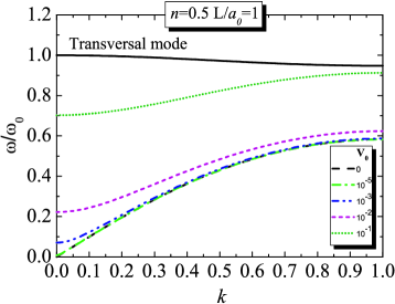
Figure 10: (Color online) The phonon spectrum for different values of $V_{0}$ in the case $n=0.5$ and $L/a_{0}=1$.

In Fig. 10(a), the phonon spectrum for the one-chain configuration is presented for different values of $V_{0}$, fixed density $n=0.5$ and $L/a_{0}=1$. In this case, there is one particle per unit cell located in each minimum of the substrate resulting only in one longitudinal mode and one transversal mode. The frequency of the longitudinal mode increases with increasing $V_{0}$, and there is a gap opening at $k=0$. The reason is that the periodic potential acts locally as a parabolic confinement potential $V(x)\simeq V_{0}\frac{2\pi^{2}}{L^{2}}x^{2}$ with frequency $\omega=\sqrt{V_{0}/m}\frac{2\pi}{L}$. The $k=0$ gap corresponds with this frequency for not too small values of $V_{0}$. The transversal mode corresponds to particle oscillations in the y-direction and is therefore practically independent of $V_{0}$.

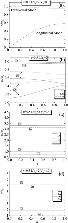
Figure 11: The phonon spectrum for different values of $V_{0}$ in the case $n=0.5$ and $L/a_{0}=2$.

In Fig. 11, the dispersion curves for $n=0.5$ and $L/a_{0}=2$ are presented for different values of $V_{0}$. As observed in Fig. 2, the presence of the substrate ($V_{0}\neq 0$) modifies the number of particles in the unit cell in order that the number of branches of the phonon spectrum is increased as compared to the case $V_{0}=0$ [Fig. 11(a)]. For $V_{0}\neq 0$ there are two particles per unit cell and consequently four branches in the phonon spectrum. As $V_{0}$ increases, the frequency of the LA mode also increases, which can be explained keeping in mind that for low values of $V_{0}$, there is a small electrostatic repulsion between neighboring particles, in order that particles oscillate horizontally without major difficulties. The opposite behavior is found for the TO mode, i.e., decreases with increasing $V_{0}$. The distance between adjacent particles in the same substrate minimum becomes smaller, and the repulsive force between them increases and acts as a retarding force.

The LO mode has a rather different behavior as compared to the TO mode, i.e., there is a hardening of its frequency when $V_{0}$ increases, which is a consequence of the larger repulsion due to the closer proximity between particles. For a sufficiently strong $V_{0}$ [ Fig. 11(c)] the normal mode spectrum becomes discrete, i.e. frequencies become independent on k, which means the group velocity is zero and the modes become localized.

As commented previously, for $V_{0}\geq 0.8$ there is a structural phase transition to the two-chain configuration with particles aligned along the y-direction (YAC phase) in each minima of the substrate [Fig. 2]. Again, due to the strong confinement the modes are localized, and a discrete spectrum is found [Fig. 11(c)] with large frequencies for the longitudinal modes. The transversal modes also present an increase in the frequency due the large confinement in the y-direction.

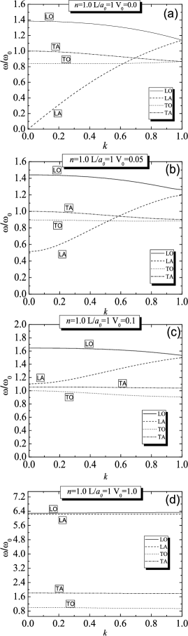
Figure 12: The phonon spectrum for different values of $V_{0}$ in the case $n=1$ and $L/a_{0}=1$.

Now we discuss the dispersion curves for the system with density $n=1.0$ and $L/a_{0}=1$, [Fig. 12]. As presented earlier [Fig. 4], particles remain in the two-chains configuration for all $V_{0}$ with changes only in the internal structure. Again the substrate potential induces gaps in the normal mode frequencies as presented in Fig. 12. The TA, TO, LA and LO modes increase with increasing $V_{0}$.

In the case of the LA mode, for low values of $V_{0}$ particles are not aligned, having more freedom to oscillate in the horizontal direction. When $V_{0}$ increases, the electrostatic force becomes larger (particles are now aligned) making oscillations along the channel harder.

The LO mode also increases with increasing $V_{0}$. This is a consequence of the strength of the substrate potential, which trap particles in their equilibrium positions, reducing the out phase oscillations of the particles. The TO frequency increases slightly, since the out-of-phase motion is more difficult to occur. The TA frequency branch is almost independent of $V_{0}$ because it corresponds to oscillations in the $y$-direction and is therefore determined by the harmonic confinement potential with frequency $\omega_{0}$.

For the YAC phase, $V_{0}>0.16$, the normal mode spectrum becomes discrete [Fig. 12(d)], as in the case $n=0.5$, $L/a=2.0$. The modes are almost constant due to the strong confinement potential imposed by the substrate and the harmonic trap.

V Conclusions

We investigated the structural and dynamical properties of a two-dimensional system of repulsive particles confined by a parabolic channel and submitted to a one-dimensional periodic potential (substrate). The ground state configurations were obtained analytically and numerically, where for the latter we used molecular dynamics simulations. The phonon spectrum were also calculated analytically for the one- and two-chain configurations through the harmonic approximation.

The main features of the structure and normal mode spectrum were studied (for different densities) as a function of the periodicity ($L$) and strength ($V_{0}$) of the substrate, which are experimentally tunable parameters in systems like e.g. colloids in the presence of a periodic light field composed of two interfering laser beams. An interesting set of ground state configurations with controllable porosity is observed mainly as a function of $V_{0}$, through several first or second order structural transitions. The structures are mainly ruled by the fact that particles tend to go to the minima of the periodic substrate, modifying the symmetry of the ordered structures. However, for small $V_{0}$ the inter particle repulsive interaction dominates and the particles are found over all possible positions in the periodic potential, including regions near to the maxima. For large $V_{0}$, particles are more and more attracted to the wells of the periodic potential.

For some specific cases we found structural transitions where the number of particles in the unit cell of the periodic system is changed, implying e.g. a different number of branches in the phonon spectrum, which is an interesting aspect of the dynamical behavior of the system, specially for applications in phononics.

The normal mode frequencies depend on the linear density of the system, periodicity and strength of the periodic substrate. We observed gaps in the phonon spectrum, which indicate that there are frequencies blocked by the crystal. For $V_{0}$ beyond a critical value and for specific values of the ratio $L/a_{0}$ the system is found in a special configuration were particles are aligned in each minimum of the periodic substrate and perpendicular to the $x$-direction. For such a configuration the normal mode frequencies become independent of the wave vector and the modes localize into a small frequency of interval.

*

Appendix A

The matrix $\omega^{2}\textbf{I}-\textbf{D}$ (where I is the unit matrix and D is the dynamical matrix) is used in the calculation of the normal modes for the one- and two-chains configurations. The dynamical matrix for one chain configuration when $V_{0}=0$ is:

$$\left[\begin{array}[]{rrrr}\omega^{2}-A_{1}&0\\ 0&(\omega^{2}-\omega_{0}^{2})-A_{2}\\ \end{array}\right],$$

where the quantities $A_{1}$ and $A_{2}$ are given by:

$$\begin{split}A_{1}&=\sum_{j=1}^{\infty}n^{3}\frac{e^{-\kappa j/n}}{j^{3}}\Big{[}2+\frac{2\kappa j}{n}+\frac{\kappa^{2}{j}^{2}}{n^{2}}\Big{]}[1-cos(k\pi{j})]\\ &+{V_{0}}{\pi n}^{2}cos(\pi j)\end{split}$$ (12)

$$A_{2}=\sum_{j=1}^{\infty}n^{3}\frac{e^{-\kappa j/n}}{j^{3}}\Big{[}1+\frac{\kappa{j}}{n}\Big{]}[1-cos(k\pi{j})]$$ (13)

The dimensionless wave number $k$ is in units of $2\pi/L$. The dynamical matrix to one-chain $V_{0}\neq 0$ and two-chains configuration is:

$$\left[\begin{array}[]{rrrr}\omega^{2}-B_{1}-sub&0&-B_{5}&0\\ 0&\Delta\omega^{2}-B_{2}&0&-B_{6}\\ -B_{7}&0&\omega^{2}-B_{3}-sub&0\\ 0&-B_{8}&0&\Delta\omega^{2}-B_{4}\\ \end{array}\right],$$

where $\Delta\omega^{2}=\omega^{2}-\omega_{0}^{2}$. The quantities $B_{1}$, $B_{2}$, $B_{3}$, $B_{4}$, $B_{5}$ and $B_{6}$ are given by:

$$\begin{split}B_{1}&=\sum_{j=1}^{\infty}n^{3}\frac{e^{-2\kappa r/n}}{(2r)^{3}}\Big{[}(j-c_{x})^{2}\Big{(}\frac{3}{r^{2}}+\frac{6\kappa}{nr}+\frac{4\kappa^{2}}{n^{2}}\Big{)}\\ &-(1+\frac{2\kappa r}{n})\Big{]}+\sum_{j=1}^{\infty}n^{3}\frac{e^{-2\kappa j/n}}{(2j)^{3}}\Big{[}2+\frac{4\kappa j}{n}+\frac{(2\kappa j)^{2}}{n^{2}}\Big{]}\\ &\times[1-exp(ikjL)]\\ \end{split}$$ (14)

$$\begin{split}B_{2}&=\sum_{j=1}^{\infty}n^{3}\frac{e^{-2\kappa r/n}}{(2r)^{3}}\Big{[}\frac{3c_{y}^{2}}{r^{2}}+\frac{4\kappa^{2}c_{y}^{2}}{n^{2}}+\frac{6\kappa c_{y}^{2}}{nr}-(1+\frac{\kappa r}{n})\Big{]}\\ &-\sum_{j=1}^{\infty}n^{3}\frac{e^{-2\kappa j/n}}{(2j)^{3}}\Big{[}1+\frac{2\kappa j}{n}\Big{]}[1-exp(ikjL)],\end{split}$$ (15)

$$\begin{split}B_{3}&=\sum_{j=1}^{\infty}n^{3}\frac{e^{-2\kappa r_{1}/n}}{(2r)^{3}}\Big{[}(j-1+c_{x})^{2}\Big{(}\frac{3}{r^{2}}+\frac{6\kappa}{nr}+\frac{4\kappa^{2}}{n^{2}}\Big{)}\\ &-(1+\frac{2\kappa r_{1}}{n})\Big{]}+\sum_{j=1}^{\infty}n^{3}\frac{e^{-2\kappa j/n}}{(2j)^{3}}\Big{[}2+\frac{4\kappa j}{n}+\frac{(2\kappa j)^{2}}{n^{2}}\Big{]}\\ &\times[1-exp(ikjL)]\\ \end{split}$$ (16)

$$\begin{split}B_{4}&=\sum_{j=1}^{\infty}n^{3}\frac{e^{-2\kappa r_{1}/n}}{(2r_{1})^{3}}\Big{[}\frac{3c_{y}^{2}}{r_{1}^{2}}+\frac{4\kappa^{2}c_{y}^{2}}{n^{2}}+\frac{6\kappa c_{y}^{2}}{nr_{1}}-(1+\frac{\kappa r_{1}}{n})\Big{]}\\ &-\sum_{j=1}^{\infty}n^{3}\frac{e^{-2\kappa j/n}}{(2j)^{3}}\Big{[}1+\frac{2\kappa j}{n}\Big{]}[1-exp(ikjL)]\end{split}$$ (17)

$$\begin{split}B_{5}&=\sum_{j=1}^{\infty}n^{3}\frac{e^{-2\kappa r/n}}{(2r)^{3}}\Big{[}(j-c_{x})^{2}\Big{(}\frac{3}{r^{2}}+\frac{6\kappa}{nr}+\frac{4\kappa^{2}}{n^{2}}\Big{)}\\ &-(1+\frac{2\kappa r}{n})\Big{]}[exp(ikL(j-c_{x}))]\\ \end{split}$$ (18)

$$\begin{split}B_{6}&=\sum_{j=1}^{\infty}n^{3}\frac{e^{-2\kappa r/n}}{(2r)^{3}}\Big{[}\frac{3c_{y}^{2}}{r^{2}}+\frac{4\kappa^{2}c_{y}^{2}}{n^{2}}+\frac{6\kappa c_{y}^{2}}{nr}-(1+\frac{\kappa r}{n})\Big{]}\\ &\times[exp(ikL(j-c_{x}))],\end{split}$$ (19)

$$\begin{split}B_{7}&=\sum_{j=1}^{\infty}n^{3}\frac{e^{-2\kappa r_{1}/n}}{(2r)^{3}}\Big{[}(j-1+c_{x})^{2}\Big{(}\frac{3}{r^{2}}+\frac{6\kappa}{nr}+\frac{4\kappa^{2}}{n^{2}}\Big{)}\\ &-(1+\frac{2\kappa r_{1}}{n})\Big{]}[exp(ikL(j+c_{x}))]\\ \end{split}$$ (20)

$$\begin{split}B_{8}&=\sum_{j=1}^{\infty}n^{3}\frac{e^{-2\kappa r_{1}/n}}{(2r_{1})^{3}}\Big{[}\frac{3c_{y}^{2}}{r_{1}^{2}}+\frac{4\kappa^{2}c_{y}^{2}}{n^{2}}+\frac{6\kappa c_{y}^{2}}{nr_{1}}-(1+\frac{\kappa r_{1}}{n})\Big{]}\\ &\times[exp(ikL(j+c_{x}))],\end{split}$$ (21)

where $r=\sqrt{(i-c_{x})^{2}+c_{y}^{2}}$, $r_{1}=\sqrt{(i-1+c_{x})^{2}+c_{y}^{2}}$, the dimensionless wave number $k$ is in units of $2\pi/L$, $i=\sqrt{-1}$ and $sub=8V_{0}\pi^{2}cos(\pi c_{x})$.

References

- (1) H. H. vonGrünberg and J. Baumgartl, Phys. Rev. E 75, 051406 (2007).
- (2) A. Chowdhury, B. J. Ackerson, and N. A. Clark, Phys. Rev. Lett. 55, 833 (1985).
- (3) C. Bechinger, M. Brunner, and P. Leiderer, Phys. Rev. Lett. 86, 930 (2001).
- (4) Reichhardt, C. J. O. and C. Reichhardt (2003). J. Phys. A: Math. Gen. 36, 5841 (2003).
- (5) C. Reichhardt and C. J. Olson, Phys. Rev. Lett. 88, 248301 (2002).
- (6) M. Mikulis, C.J. Olson Reichhardt, C. Reichhardt, R.T. Scalettar, and G.T. Zim anyi, J. Phys: Condens. Matter 16, 7909 (2004).
- (7) M. Brunner and C. Bechinger, Phys. Rev. Lett. 88, 248302 (2002).
- (8) A. M. Alsayed, M. F. Islam, J. Zhang, P. J. Collings, and A. G. Yodh, Science, 309, 1207 (2005).
- (9) S. Herrera-Velarde and R. Castaneda-Priego, J. Phys.: Condens. Matter 19, 226215 (2007).
- (10) S. Herrera-Velarde and R. Castaneda-Priego, Phys. Rev. E 77, 041407 (2008).
- (11) V. M. Bedanov and F. M. Peeters, Phys. Rev. B 49, 2667 (1994).
- (12) J. H. Chu and Lin I, Phys. Rev. Lett. 72, 4009 (1994).
- (13) Bin Liu, K. Avinash, and J. Goree, Phys. Rev. Lett. 91, 255003 (2003).
- (14) Bin Liu and J. Goree, Phys. Rev. E 71, 046410 (2005).
- (15) K. Zahn, R. Lenke, and G. Maret, Phys. Rev. Lett. 82, 2721 (1999).
- (16) M. Golosovsky, Y. Saado, and D. Davidov, Phys. Rev. E 65, 061405 (2002).
- (17) P. Glasson, V. Dotsenko, P. Fozooni, M. J. Lea, W. Bailey, G. Papageorgiou, S.E. Andresen, and A. Kristensen, Phys. Rev. Lett. 87, 176802 (2001).
- (18) David Rees and Kimitoshi Kono, J. Low Temp. Phys. 158, (2010).
- (19) A. Homann, A. Melzer, S. Peters, and A. Piel, Phys. Rev. E 56, 7138 (1997)
- (20) T. Misawa, N. Ohno, K. Asano, M. Sawai, S. Takamura, and P. K. Kaw, Phys. Rev. Lett. 86, 1219 (2001).
- (21) B. Liu and J. Goree, Phys. Rev. E 71, 046410 (2005).
- (22) A. Melzer, Phys. Rev. E 73, 056404 (2006).
- (23) T. E. Sheridan and K. D. Wells , Phys. Rev. E 81, 016404 (2010).
- (24) M. Köppl, P. Henseler, A. Erbe, P. Nielaba, and P. Leiderer, Phys. Rev. Lett. 97, 208302 (2006).
- (25) K. Mangold, J. Birk, P. Leiderer, and C. Bechinger, Phys. Chem. Chem. Phys., 6, 20041623
- (26) G. Piacente, I. V. Schweigert, J. J. Betouras, and F. M. Peeters, Phys. Rev. B 69, 045324 (2004).
- (27) G. Piacente, G. Q. Hai, and F. M. Peeters, Phys. Rev. B 81, 024108 (2010).
- (28) W. P. Ferreira, J. C. N. Carvalho, P. W. S. Oliveira, G. A. Farias, and F. M. Peeters, Phys. Rev. B 77, 014112 (2008).
- (29) W. P. Ferreira, G. A. Farias, and F. M. Peeters, to appear in J. Phys.: Condens. Matter
- (30) L. Candido, J.P. Rino, N. Studarta, and F.M. Peeters, J. Phys.: Condens. Matter 10, 11627 (1998).
- (31) P. M. Chaikin, and T. C. Lubensky, Cambridge University Press; 1st edition, ISBN 0521794501, Principles of Condensed Matter Physics (2000).
- (32) Jia Ou, Samuel J. Carpenter, and Kevin D. Dorfman, Biomicrofluidics 4, 013203 (2010).
- (33) P. S. Doyle, J. Bibette, A. Bancaud, and J.-L. Viovy, Science 295, 2237 (2002).
- (34) H. Löwen, J. Phys.: Condens. Matter 13, R415 (2001).
- (35) A. Yethiraj and A. Van Blaaderen, Nature (London) 421, 513 (2003).