Enhanced Compressive Wideband Frequency Spectrum Sensing for Dynamic Spectrum Access

Abstract

Wideband spectrum sensing detects the unused spectrum holes for dynamic spectrum access (DSA). Too high sampling rate is the main problem. Compressive sensing (CS) can reconstruct sparse signal with much fewer randomized samples than Nyquist sampling with high probability. Since survey shows that the monitored signal is sparse in frequency domain, CS can deal with the sampling burden. Random samples can be obtained by the analog-to-information converter. Signal recovery can be formulated as an L0 norm minimization and a linear measurement fitting constraint. In DSA, the static spectrum allocation of primary radios means the bounds between different types of primary radios are known in advance. To incorporate this a priori information, we divide the whole spectrum into subsections according to the spectrum allocation policy. In the new optimization model, the minimization of the L2 norm of each subsection is used to encourage the cluster distribution locally, while the L0 norm of the L2 norms is minimized to give sparse distribution globally. Because the L0/L2 optimization is not convex, an iteratively re-weighted L1/L2 optimization is proposed to approximate it. Simulations demonstrate the proposed method outperforms others in accuracy, denoising ability, etc.

I Introduction

Cognitive radio (CR) is a very promising technology for wireless communication. Radio spectrum is a precious natural resource. The fixed spectrum allocation is the major way for the spectrum allocation now. In order to avoid interference, different wireless services are allocated with different licensed bands. Currently most of the available spectrum has been allocated. But the increasing wireless services, especially the wideband ones, call for much more spectrum access opportunities. The allocated spectrum becomes very crowded and spectrum scarcity comes. To deal with the spectrum scarcity problem, there are several ways, such as multiple-input and multiple-output (MIMO) communication [1], ultra-wideband (UWB) communication [2], beamforming [3] [4], relay [5], and so on. Investigation demonstrates that most of the allocated bands are in very low utility ratios [6]. CR is proposed to exploit the under-utilization of the radio frequency (RF) spectrum. It is a paradigm in which the cognitive transmitter changes its parameters to avoid interference with the licensed users. This alteration of parameters is based on the timely monitoring of the factors in the radio environment.

Spectrum sensing is one of the main functions of CR. It detects the unused frequency bands, and then CR users can be allowed to utilize the unused primary frequency bands. Current spectrum sensing is performed in two steps [7]: the first step called coarse spectrum sensing is to efficiently detect the power spectrum density (PSD) level of primary bands; the second step, called feature detection or multi-dimensional sensing [8], is to estimate other signal space accessible for CR, such as direction of arrival (DOA) estimation, spread spectrum code identification, waveform identification, etc.

Coarse spectrum sensing requires fast and accurate power spectrum detection over a wideband and even ultra-wideband (UWB). One approach utilizes a bank of tunable narrowband bandpass filters. But it requires an enormous number of RF components and bandpass filters, which leads to high cost. Besides, the number of the bands is fixed and the filter range is always preset. Thus the filter bank way is not flexible. The other one is a wideband circuit using a single RF chain followed by high-speed digital signal processor (DSP) to flexibly search over multiple frequency bands concurrently [9]. It is flexible to dynamic power spectrum density. High sampling rate requirement and the resulting large number of data for processing are the major problems [10].

Too high sampling rate requirement brings challenge to the analog-to-digital converter (ADC). And the resulting large amount of data requires large storage space and heavy computation burden of DSP. Since survey shows sparsity exists in the frequency domain for primary signal, compressive sensing (CS) can be used to effectively decrease the sampling rate [11] [12] [13]. It assets that a signal can be recovered with a much fewer randomized samples than Nyquist sampling with high probability on condition that the signal has a sparse representation.

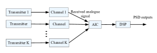
Figure 1: The proposed compressive wideband spectrum sensing structure.

In compressive wideband spectrum sensing (CWSS), analog-to-information converter (AIC) can be taken to obtain the random samples from analog signal in hardware as Fig. 1 shows [14] [15]. To get the spectrum estimation, there are mainly two groups of methods [13]. One group is convex relaxation, such as basis pursuit (BP) [16] [17], Dantzig Selector (DS) [18] , and so on; the other is greedy algorithm, such as matching pursuit (MP) [19], orthogonal matching pursuit (OMP) [20], and so on. Both of the convex programming and greedy algorithm have advantages and disadvantages when applied to different scenarios. A short assessment of their differences would be that convex programming algorithm has a higher reconstruction accuracy while greedy algorithm has less computation complexity. In contrast to BP, basis pursuit denoising (BPDN) has better denoising performance [17] [21].

In this paper, the partial Fourier random samples are obtained via AIC with the measurement matrix generated by choosing part of separate rows randomly from the Fourier sampling matrix [14]. Based on the random samples, a generalized sparse constraint in the form of mixed $\mathscr{C}_{2}$/$\mathscr{C}_{1}$ norm is proposed to enhance the recovery performance by exploiting the structure information. It encourages locally cluster distribution and globally sparse distribution. In the constraint, the estimated spectrum vector is divided into sections with different length according to the a priori information about fixed spectrum allocation. The sum of weighted $\mathscr{C}_{2}$ norms of the sections is minimized. The weighting factor is iteratively updated as the reciprocal of the energy in the corresponding subband to get more democratical penalty of nonzero coefficients. Simulation results demonstrate that the proposed generalized sparse constraint based CWSS gets better performance than the traditional methods in spectrum reconstruction accuracy.

In the rest of the paper, Section II gives the signal model; Section III states the classical CWSS methods. Section IV provides the generalized sparse constraint based CWSS methods; In section V, the performance enhancement of the proposed method is demonstrated by numerical experiments; Finally Section VI draws the conclusion.

II Signal Model

According to the FCC report [6], the allocated spectrum is in a very low utilization ratio. It means the spectrum is in sparse distribution. Recently a survey of a wide range of spectrum utilization across 6 GHz of spectrum in some palaces of New York City demonstrated that the maximum utilization of the allocated spectrum is only 13.1$\%$. It is also the reason that CR can work. Thus it is reasonable that only a small part of the constituent signals will be simultaneously active at a given location and a certain range of frequency band. The sparsity inherently exists in the wideband spectrum [10] [22] [23] [24] [25] [26] [27] [28].

An ${N\times 1}$ signal vector x can be expanded in an orthogonal complete dictionary ${\bf{\Psi}}_{N\times N}$, with the representation as

$${\bf{x}}_{N\times 1}={\bf{\Psi}}_{N\times N}{\bf{b}}_{N\times 1}$$ (1)

When most elements of the ${N\times 1}$ vector b are zeros, the signal x is sparse. When the number of nonzero elements of b is S (S $\ll$ M $<$ N), the signal is said to be S-sparse.

In traditional Nyquist sampling, the time window for sensing is $t\in[0,T_{0}]$. N samples are needed to recover the frequency spectrum r without aliasing, where $T_{0}$ is the Nyquist sampling duration. A digital receiver converts the continuous signal x(t) to a discrete complex sequence $\textbf{y}_{t}$ of length M. For illustration convenience, we formulate the sampling model in discrete setting as it does in [10] [22] [23] [24] [25] [26] [27] [28]:

$${\bf{y}}_{t}={\bf{Ax}}_{t}$$ (2)

where $\textbf{x}_{t}$ represents an $N\times 1$ vector with elements $x_{t}[n]=x(t),~{}t=nT_{0},~{}n=1,\cdots,N$, and A is an $M\times N$ projection matrix. For example, when $\textbf{A}=\textbf{F}_{N}$ with M = N, model (2) amounts to frequency domain sampling, where $\textbf{F}_{N}$ is the N-point unitary discrete Fourier transform (DFT) matrix. Given the sample set $\textbf{x}_{t}$ when $M<N$, compressive spectrum sensing can reconstruct the spectrum of r(t) with the reduced amount of sampling data.

To monitor such a broad band, high sampling rate is needed. It is often very expensive. Besides, too many sampling measurements inevitably ask more storage devices and result in high computation burden for digital signal processors (DSP), while spectrum sensing should be fast and accurate. CS provides an alternative to the well-known Nyquist-Shannon sampling theory. It is a framework performing non-adaptive measurement of the informative part of the signal directly on condition that the signal is sparse [13]. Since it is proved that $\textbf{x}_{t}$ has a sparse representation in frequency domain. We can use an $M\times N$ random projection matrix $\textbf{S}_{c}$ to sample signals, i.e. ${\bf{y}}_{t}={\bf{S}}_{c}{\bf{x}}_{t}$, where $M<N$; $\textbf{S}_{c}$ is a non-uniform subsampling or random subsampling matrix which is generated by choosing M separate rows randomly from the unit matrix $\textbf{I}_{N}$.

The AIC can be used to sample the analog baseband signal x(t). One possible architecture can be based on a wideband pseudorandom demodulator and a low rate sampler [14] [15]. First we modulate the analogue signal by a pseudo-random maximal-length PN sequence. Then a low-pass filter follows. Finally, the signal is sampled at sub-Nyquist rate using a traditional ADC. It can be conceptually modeled as an ADC operating at Nyquist rate, followed by random discrete sampling operation [14]. Then $\textbf{y}_{t}$ is obtained directly from continuous time signal x(t) by AIC. The details about AIC can be found in [14] [15]. Here we incorporate the AIC to the spectrum sensing architecture as Fig. 1 shows.

III The Classical Compressive Wideband Spectrum Sensing

CS theory asserts that, if a signal has a sparse representation in a certain space, one can use the random sampling to obtain the measurements and successfully reconstruct the signal with overwhelming probability by nonlinear algorithms, as stated in section II. The required random samples for recovery are far fewer than Nyquist sampling.

To find the unoccupied spectrum for secondary access, the signal in the monitored band is down-converted to baseband. The analog baseband signal is sampled via the AIC that produces measurements at a rate below the Nyquist rate.

Now we estimate the frequency response of x(t) from the measurement vector $\textbf{y}_{t}$ based on the transformation equality ${\bf{y}}_{t}={\bf{S}}_{c}{\bf{F}}_{N}^{-1}{\bf{r}}$, where r is the $N\times 1$ frequency response vector (FRV) of signal x(t); $\textbf{F}_{N}$ is the $N\times N$ Fourier transform matrix; $\textbf{S}_{c}$ is the $M\times N$ matrix which is obtained by randomizing the column indices and getting the first M columns.

Under the sparse spectrum assumption, the FRV can be recovered by solving the combinatorial optimization problem

$$\begin{array}[]{c}{\rm{}}{\bf{\hat{r}}}=\mathop{\arg\min}\limits_{\bf{r}}\left\|{\bf{r}}\right\|_{0}\\ {\rm{s}}{\rm{.~{}t}}{\rm{.~{}~{}}}\left({{\bf{S}}_{c}^{T}{\bf{F}}_{M}^{-1}}\right){\bf{r}}={\bf{y}}_{t}\\ \end{array}$$ (3)

Since the optimization problem (3) is nonconvex and generally impossible to solve, for its solution usually requires an intractable combinatorial search. As it does in [10], BP is used to recover the signal:

$$\begin{array}[]{l}{\rm{}}{\bf{r}}_{BP}=\mathop{\arg\min}\limits_{\bf{r}}\left\|{\bf{r}}\right\|_{1}\\ {\rm{s}}{\rm{.~{}t}}{\rm{.~{}~{}}}\left({{\bf{S}}_{c}^{T}{\bf{F}}_{M}^{-1}}\right){\bf{r}}={\bf{y}}_{t}\\ \end{array}$$ (4)

This problem is a second order cone program (SOCP) and can therefore be solved efficiently using standard software packages.

BP finds the smallest $\mathscr{C}_{1}$ norm of coefficients among all the decompositions that the signal is decomposed into a linear combination of dictionary elements (columns, atoms). It is a decomposition principle based on a true global optimization.

In practice noise exists in data. Another algorithm called BPDN has superior denoising performance than BP [21]. It is a shrinkage and selection method for linear regression. It minimizes the sum of the absolute values of the coefficients, with a bound on the sum of squared errors. To get higher accuracy, we can formulate the BPDN based compressive wideband spectrum sensing (BPDN-CWSS) optimization model as:

$$\begin{array}[]{c}{\rm{}}{\bf{r}}_{BPDN}=\mathop{\arg\min}\limits_{\bf{r}}\left\|{\bf{r}}\right\|_{1}\\ {\rm{s}}{\rm{.~{}t}}{\rm{.~{}~{}}}\left\|{\left({{\bf{S}}_{c}^{T}{\bf{F}}_{M}^{-1}}\right){\bf{r}}-{\bf{y}}_{t}}\right\|_{2}\leq\eta_{1}\\ \end{array}$$ (5)

where $\eta_{1}$ bounds the amount of noise in the data. The computation of the BPDN is a quadratic programming problem or more general convex optimization problem, and can be done by classical numerical analysis algorithms. The solution has been well investigated [21] [29] [30] [31]. A number of convex optimization software, such as cvx [32], SeDuMi [33] and Yalmip [34], can be used to solve the problem.

IV The Proposed Compressive Wideband Spectrum Sensing

Among the classical sparse signal recovery algorithms, BPDN achieves the highest recovery accuracy [13]. However, it only takes advantage of sparsity. In wideband CR application, additional a priori information about the spectrum structure can be obtained. The further exploitation of structure information would give birth to recovery accuracy enhancement [28] [35] [36] . Besides, It is well-known that the minimization of $\mathscr{C}_{0}$ norm is the best candidate for sparse constraint. But in order to reach a convex programming, the $\mathscr{C}_{0}$ norm is relaxed to $\mathscr{C}_{1}$ norm, which leads to the performance degeneration [37]. Here a weighting formulation is designed to democratically penalize the elements. It suggests that large weights could be used to discourage nonzero entries in the recovered FRV, while small weights could be used to encourage nonzero entries. To get the weighted values, a simple iterative algorithm is proposed.

IV-A Wideband spectrum sensing for fixed spectrum allocation

The classical algorithms reconstruct the commonly sparse signal. However, in the coarse wideband spectrum sensing, the boundaries between different kinds of primary users are fixed due to the static frequency allocation of primary radios. For example, the bands 1710 - 1755 MHz and 1805 - 1850 MHz are allocated to GSM1800. Previous CWSS algorithms did not take advantage of the information of fixed frequency allocation boundaries. Besides, according to the practical measurement, though the spectrum vector is sparse globally, in some certain allocated frequency sections, they are not always sparse. For example, in a certain time and area, the frequency sections 1626.5 - 1646.5 MHz and 1525.0 - 1545.0 MHz allocated to international maritime satellite are not used, but the frequency sections allocated to GSM1800 are fully occupied. The wideband FRV is not only sparse, but also in sparse cluster distribution with different length of clusters. It is the generalization of the so called block-sparsity [35] [36]. This feature is extremely vivid in the situation that most of the monitored primary signals are spread spectrum signals.

Previous classical CWSS does not assume any additional structure on the unknown sparse signal. However in the practical application, the signal may have other structures. Incorporating additional structure information would improve the recoverability potentially.

Block-sparse signal is the one whose nonzero entries are contained within several clusters. To exploit the block structure of ideally block-sparse signals, $\mathscr{C}_{2}$/$\mathscr{C}_{1}$ optimization was proposed. The standard block sparse constraint (SBSC) in the form of $\mathscr{C}_{2}$/$\mathscr{C}_{1}$ optimization can be formulated as [35] [36]:

$$\begin{array}[]{c}\mathop{\min}\limits_{\bf{r}}\left({\sum\limits_{i=1}^{K}{\left\|{{\bf{r}}_{(i-1)d_{0}:id_{0}}}\right\|_{2}}}\right)\\ {\rm{s}}{\rm{.~{}t}}{\rm{.~{}~{}}}\left({{\bf{S}}_{c}^{T}{\bf{F}}_{M}^{-1}}\right){\bf{r}}={\bf{y}}_{t}\\ \end{array}$$ (6)

where K is the number of the divided subbands; $d_{0}$ is the length of the divided blocks. Extensive performance evaluations and simulations have demonstrated that as $d_{0}$ grows the algorithm significantly outperforms standard BP algorithm [36].

However, in the standard $\mathscr{C}_{2}$/$\mathscr{C}_{1}$ optimization, the estimated sparse signal is divided with the same block length, which mismatches the practical situation that the values of the length of the spectrum subbands allocated to different radios can not be all the same. Besides, the constraint in (6) does not incorporate the denoising function.

To further enhance the performance of CWSS, the fixed spectrum allocation information can be incorporated in the CWSS algorithm. Based on the a priori information about boundaries, the estimating PSD vector is divided into sections with their edges in accordance with the boundaries of different types of primary users by fixed spectrum allocation. In the BPDN-CWSS, the minimization of the standard $\mathscr{C}_{1}$-norm constraint on the whole FRV is replaced by the minimization of the sum of the $\mathscr{C}_{2}$ norm of each divided section of the FRV to encourage the sparse distribution globally while blocked distribution locally. As it combines $\mathscr{C}_{1}$ norm and $\mathscr{C}_{2}$ norm to enforce the sparse blocks with different block lengths, the new CWSS model, in the name of variable-length-block-sparse constraint based compressive wideband spectrum sensing (VLBS-CWSS), can be formulated as:

$$\begin{array}[]{c}\mathop{\min}\limits_{\bf{r}}\left({\left\|{{\bf{r}}_{1}}\right\|_{2}+\left\|{{\bf{r}}_{2}}\right\|_{2}+\cdots\left\|{{\bf{r}}_{K}}\right\|_{2}}\right)\\ {\rm{s}}{\rm{.~{}t}}{\rm{.~{}~{}}}\left\|{{\bf{y}}_{t}-{\bf{S}}_{c}{\bf{F}}_{N}^{-1}{\bf{r}}}\right\|_{2}\leq\eta_{2}\\ \end{array}$$ (7)

where $\textbf{r}_{1}$, $\textbf{r}_{2}$, … , $\textbf{r}_{K}$ are K sub-vectors of r corresponding to $d_{1}$, $d_{1}$, … , ${d_{K-1}}$ which are the boundaries of the divided sections. $\eta_{2}$ bounds the amount of noise in the data. It can be formulated as:

$${\bf{r}}=\left({\begin{array}[]{*{20}c}{\underbrace{\begin{array}[]{*{20}c}{r_{1}}&\cdots&{r_{d_{1}}}\\ \end{array}}_{{\bf{r}}_{1}}}&\cdots&{\underbrace{\begin{array}[]{*{20}c}{r_{d_{K-1}+1}}&\cdots&{r_{N}}\\ \end{array}}_{{\bf{r}}_{K}}}\\ \end{array}}\right)^{T}$$ (8)

Since the objective function in the VLBS-CWSS (7) is convex and the other constraint is an affine, it is a convex optimization problem. It can also be solved by a host of numerical methods in polynomial time. Similar to the solution of the BPDN-CWSS (5), the optimal r of the VLBS-CWSS (7) can also be obtained efficiently using some convex programming software packages. Such as cvx [32], SeDuMi [33], and Yalmip [34], etc.

After we get r from (8), power spectrum can be obtained. Several ways can indicate the spectrum holes, such as energy detection [27], edge detection [10], and so on. For example, in energy detection we will calculate ${\left\|{{{\bf{r}}_{k}}}\right\|_{2}}$, k = 1, 2, … , K. Comparing it with an experimental threshold, the spectrum holes for dynamic access can be clearly given. The energy detection will be used in numerical simulations.

IV-B Enhanced variable-length-block-sparse spectrum sensing

In sparse constraint, $\mathscr{C}_{0}$ norm minimization is relaxed to $\mathscr{C}_{1}$ norm at the cost of bringing the dependence on the magnitude of the estimated vector. In the $\mathscr{C}_{1}$ norm minimization, larger entries are penalized more heavily than smaller ones, unlike the more democratic penalization of the $\mathscr{C}_{0}$ norm. Here in the the VLBS constraint, to encourage sparse distribution of the spectrum in the global perspective, the $\mathscr{C}_{1}$ norm of a series of the $\mathscr{C}_{2}$ norm is minimized. Similarly, the dependence on the power in each subband exits.

To deal with this imbalance, the minimization of the weighted sum of the $\mathscr{C}_{2}$ norm of each blocks is designed to more democratically penalize. The new weighted VLBS constraint based compressive wideband spectrum sensing (WVLBS-CWSS) can be formulated as:

$$\begin{array}[]{c}\mathop{\min}\limits_{\bf{r}}\left({w_{1}\left\|{{\bf{r}}_{1}}\right\|_{2}+w_{2}\left\|{{\bf{r}}_{2}}\right\|_{2}+\cdots+w_{K}\left\|{{\bf{r}}_{K}}\right\|_{2}}\right)\\ {\rm{s}}{\rm{.t}}{\rm{.}}\left\|{{\bf{y}}_{t}-{\bf{S}}_{c}{\bf{F}}_{N}^{-1}{\bf{r}}}\right\|_{2}\leq\eta_{3}\\ \end{array}$$ (9)

where $\textbf{r}_{1}$, $\textbf{r}_{2}$, … , $\textbf{r}_{K}$ are defined as (8); $\eta_{3}$ bounds the amount of noise; ${\bf{w}}=\left[{\begin{array}[]{*{20}c}{w_{1}}&{w_{2}}&\cdots&{w_{K}}\\ \end{array}}\right]^{T}$. $w_{i}$ depends on $p_{i}\geq 0,{\rm{for}}~{}i=1,\cdots,K$, where $p_{i}$ corresponds to the power of the primary user exists in the i-th subband.

Obviously, the object function of the WVLBS-CWSS (9) is convex. It is a convex optimization problem. In principle this problem is solvable in polynomial time.

To realize the WVLBS-CWSS (9), the weighting vector w should be provided. As it is defined before, the computation of the weight $w_{i}$ is in fact the computation of the $p_{i}$. Here a practical way to iteratively set the $p_{i}$ is proposed. At each iteration, the $p_{i}$ is the sum of the absolute value of frequency spectrum vector in the corresponding subband. It can be formulated as:

$$\begin{array}[]{c}p_{t,i}=\left\|{{\bf{r}}_{t-1,i}}\right\|_{1}\\ =\left|{r_{t-1,~{}d_{i-1}+1}}\right|+\cdots+\left|{r_{{t-1},~{}d_{i}}}\right|\\ \end{array}$$ (10)

where ${\bf{r}}_{t-1,~{}i}$ is the i-th sub-vector as in (8) at the (t-1)-th iteration; $r_{{t-1},~{}d_{i-1}+1},~{}\cdots~{},~{}r_{t-1,d_{i}}$ are the elements of the sub-vector ${\bf{r}}_{t-1,i}$. After getting the $p_{i}$, the weighting vector w can be formulated. Here we can get it by

$$w_{i}=\frac{1}{{p_{i}+\delta}}$$ (11)

where a small parameter $\delta>0$ in (11) is introduced to provide stability and to ensure that a zero-valued component in $p_{i}$ does not strictly prohibit a nonzero estimate at the next step.

The initial condition of the recursive relation is $w_{i}=1$, for all $i=1,...,K$. That means in the first step, all the blocks are weighted equally. Along with the increase of the iteration times, larger values of $p_{i}$ are penalized lighter in the WVLBS-CWSS (9) than smaller values of $p_{i}$. To terminate the iteration at the proper time, the stopping rule can be formulated as

$$\left\|{{\bf{r}}_{t}-{\bf{r}}_{t-1}}\right\|_{2}\leq\varepsilon$$ (12)

where ${{\bf{r}}_{t}}$ is the estimated FRV at the t-th iteration; $\varepsilon$ bounds the iteration residual.

The initial state of the iterative algorithm is the same with the VLBS-CWSS (7). To make a difference, The iterative reweighted algorithm is named as enhanced variable-length-block-sparse constraint based compressive wideband spectrum sensing (EVLBS-CWSS).

V Simulation Results

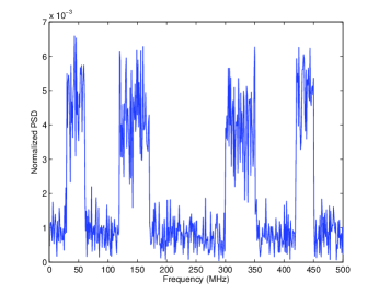
Figure 3: The normalized spectrum of noisy active primary signals in the monitoring band.

Numerical experiments are presented to illustrate performance improvement of the proposed EVLBS-CWSS for CR. Here we consider a base band signal with its frequency range from 0 Hz to 500 MHz as Fig. 2 shows. The primary signals with random phase are contaminated by a zero-mean additive white Gaussian noise (AWGN) which makes the signal to noise ratio (SNR) be 11.5 dB. Four primary signals are located at 30 MHz - 60 MHz, 120 MHz - 170 MHz, 300 MHz - 350 MHz, 420 MHz - 450 MHz. Their corresponding frequency spectrum levels fluctuate in the range of 0.0023 - 0.0066, 0.0016 - 0.0063, 0.0017 - 0.0063, and 0.0032 - 0.0064, as Fig. 3 shows. Here we take the noisy signal as the received signal x(t). As CS theory suggests, we sample x(t) randomly at the subsampling ratio 0.40 via AIC as Fig. 1. The resulted sub-sample vector is denoted as $\textbf{y}_{t}$.

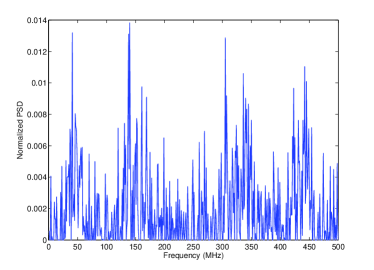
Figure 4: The compressive wideband spectrum estimation via BPDN-CWSS.

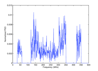
Figure 5: The compressive wideband spectrum estimation via VLBS-CWSS.

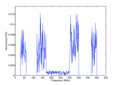
Figure 6: The compressive wideband spectrum estimation via EVLBS-CWSS.

To make contrast, with the same number of samples, The amplitude of frequency spectrum estimated by different methods are given in Fig. 4, Fig.5 and Fig. 6. Fig. 4 shows the result estimated by the standard BPDN-CWSS (5) where $\eta_{1}$ is chosen to be $0.1\left\|{{\bf{y}}_{t}}\right\|_{2}$ with 1000 tries averaged; Fig. 5 does it by the VLBS-CWSS (7) where $\eta_{2}$ is chosen to be $0.2\left\|{{\bf{y}}_{t}}\right\|_{2}$; Fig. 6 does it by the proposed EVLBS-CWSS (9) where $\eta_{3}$ is chosen to be $0.2\left\|{{\bf{y}}_{t}}\right\|_{2}$, and $\delta$ is chosen to be 0.001.

Fig. 6 shows that the proposed EVLBS-CWSS gives the best reconstruction performance. It shows that there are too many fake spectrum points in the subbands with no active primary signal in Fig 4 which is given by the standard BPDN. The noise levels of the spectrum estimated by the B-CWSS and the VLBS-CWSS are high along the whole monitored band. For the VLBS-CWSS, as in Fig. 5, it has considerable performance improvement, but the noise level in part of the inactive subbands is still high. Some of the estimated spectrum in the inactive subband is a little too high. However, in Fig. 6, the four occupied bands clearly show up; the noise levels in the inactive bands are quite low; the variation of the spectrum levels in the boundaries of estimated spectrum are quite abrupt and correctly in accordance with the generated sparse spectrum in Fig. 2, which would enhance the edge detection performance much. Therefore, the proposed EVLBS-CWSS outperforms the standard BPDN-CWSS and the VLBS-CWSS for wideband spectrum sensing.

Apart from the edge detection, energy detection is the most popular spectrum sensing approach for CR. To test the CWSS performance by energy detection, 1000 Monte Carlo simulations are done with the same parameters above to give the results of average energy in each section of the divided spectrum vector with the BPDN-CWSS (5), the VLBS-CWSS (7) and the EVLBS-CWSS (9). The parameter setting is same as before. The simulated monitored band is divided into 9 sections as Fig 2. The total energy with each CWSS method is normalized. Table Enhanced Compressive Wideband Frequency Spectrum Sensing for Dynamic Spectrum Access presents the average energy in each subband with different recovery methods, when there are 4 active bands and the sub-sampling ratio is 0.40; Table Enhanced Compressive Wideband Frequency Spectrum Sensing for Dynamic Spectrum Access does when there are 3 active bands and the sub-sampling ratio is 0.40; Table Enhanced Compressive Wideband Frequency Spectrum Sensing for Dynamic Spectrum Access does when there are 3 active bands and the sub-sampling ratio is 0.35; Table Enhanced Compressive Wideband Frequency Spectrum Sensing for Dynamic Spectrum Access when there are 2 active bands and the sub-sampling ratio is 0.30. For the EVLBS-CWSS, it is obvious that the estimated noise energy of inactive bands is much smaller that the other two. To quantify the performance gain of EVLBS-CWSS against others, after normalizing the total energy of the spectrum vectors, we define the energy detection performance enhancement ratios (EDPER) of VLBS-CWSS and EVLBS-CWSS against BPDN-CWSS for the k-th subband as:

$$R1\left(k\right)=\left\{{\begin{array}[]{*{20}c}{\frac{{\left\|{{\bf{r}}_{k}^{VLBS}}\right\|_{2}^{2}-\left\|{{\bf{r}}_{k}^{BPDN}}\right\|_{2}^{2}}}{{\left\|{{\bf{r}}_{k}^{BPDN}}\right\|_{2}^{2}}},~{}~{}{\rm{for~{}active~{}subbands}}}\\ {\frac{{\left\|{{\bf{r}}_{k}^{BPDN}}\right\|_{2}^{2}-\left\|{{\bf{r}}_{k}^{VLBS}}\right\|_{2}^{2}}}{{\left\|{{\bf{r}}_{k}^{BPDN}}\right\|_{2}^{2}}},~{}~{}{\rm{for~{}inactive~{}subbands}}}\\ \end{array}}\right.$$ (13)

$$R2\left(k\right)=\left\{{\begin{array}[]{*{20}c}{\frac{{\left\|{{\bf{r}}_{k}^{EVLBS}}\right\|_{2}^{2}-\left\|{{\bf{r}}_{k}^{BPDN}}\right\|_{2}^{2}}}{{\left\|{{\bf{r}}_{k}^{BPDN}}\right\|_{2}^{2}}},~{}{\rm{for~{}active~{}subbands}}}\\ {\frac{{\left\|{{\bf{r}}_{k}^{BPDN}}\right\|_{2}^{2}-\left\|{{\bf{r}}_{k}^{EVLBS}}\right\|_{2}^{2}}}{{\left\|{{\bf{r}}_{k}^{BPDN}}\right\|_{2}^{2}}},~{}{\rm{for~{}inactive~{}subbands}}}\\ \end{array}}\right.$$ (14)

where ${{\bf{r}}_{k}^{EVLBS}}$, ${{\bf{r}}_{k}^{VLBS}}$ and ${{\bf{r}}_{k}^{BPDN}}$ represent values of estimated frequency spectrum vectors in the k-th subband via EVLBS-CWSS, VLBS-CWSS and BPDN-CWSS, respectively. These performance functions can quantify how much energy increased to enhance the probability of correct energy detection of the active primary bands and how much denoising performance is enhanced. The values of EDPER in Table Enhanced Compressive Wideband Frequency Spectrum Sensing for Dynamic Spectrum Access, Table Enhanced Compressive Wideband Frequency Spectrum Sensing for Dynamic Spectrum Access, Table Enhanced Compressive Wideband Frequency Spectrum Sensing for Dynamic Spectrum Access and Table Enhanced Compressive Wideband Frequency Spectrum Sensing for Dynamic Spectrum Access clearly tell the improvement of the proposed EVLBS-CWSS against VLBS-CWSS and BPDN-CWSS methods.

To further evaluate the performance of EVLBS-CWSS, when the number of active bands is 4 and sub-sampling ratio is 0.40, the residuals $\left\|{{\bf{r}}_{t}-{\bf{r}}_{t-1}}\right\|_{2}$ for 1000 Monte Carlo simulations are measured. Using the unnormalized received signal, the measured average power of the random samples $\textbf{y}_{t}$ is 29533. From t = 2 to t = 8, the residuals are 361.5066, 261.6972, 55.0035, 17.9325, 15.0799, 13.4075 and 12.6189. It shows the iteration is almost convergent at t = 5. The iteration would bring the increase of computation complexity, but the performance enhancement is obvious and worthwhile.

The enhancement of spectrum estimation accuracy qualifies the proposed EVLBS-CWSS as an excellent candidate for CWSS.

VI Conclusion

In this paper, CS is used to deal with the too high sampling rate requirement problem in the wideband spectrum sensing for CR. The sub-Nyquist random samples is obtained via the AIC with the partial Fourier random measurement matrix. Based on the random samples, incorporating the a priori information of the fixed spectrum allocation, an improved sparse constraint with different block length is used to enforce locally block distribution and globally sparse distribution of the estimated spectrum. The new constraint matches the practical spectrum better. Furthermore, the iterative reweighting is used to alleviate the performance degeneration when the $\mathscr{C}_{2}$/$\mathscr{C}_{0}$ norm minimization is relaxed to the $\mathscr{C}_{2}$/$\mathscr{C}_{1}$ one. Because the a priori information about boundaries of different types of primary users is added and iteration is used to enhance the VLBS constraint performance, the proposed EVLBS-CWSS outperforms previous CWSS methods. Numerical simulations demonstrate that the EVLBS-CWSS has higher spectrum sensing accuracy, better denoising performance, etc.

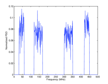
Figure 2: The normalized spectrum of noiseless active primary signals in the monitoring band.

	1	2	3	4	5	6	7	8	9
Real PSD	0	0.4747	0	0.5303	0	0.5107	0	0.4823	0
BPDN-CWSS	0.1149	0.3820	0.1752	0.4734	0.3184	0.4780	0.2333	0.4026	0.1994
VLBS-CWSS	0.0000	0.2447	0.0000	0.5101	0.4220	0.5833	0.0005	0.4020	0.0000
EVLBS-CWSS	0.0000	0.2681	0.0000	0.5396	0.1897	0.6361	0.0000	0.4431	0.0000
R1	100 $\%$	-35.94 $\%$	100 $\%$	7.75 $\%$	-32.54 $\%$	22.03 $\%$	100 $\%$	0.15 $\%$	100 $\%$
R2	100 $\%$	-29.82 $\%$	100 $\%$	13.98 $\%$	40.42 $\%$	33.08 $\%$	100 $\%$	10.06 $\%$	100 $\%$

	1	2	3	4	5	6	7	8	9
Real PSD	0.0000	0.0000	0.0000	0.5998	0.0000	0.6171	0.0000	0.5093	0.0000
BPDN-CWSS	0.2489	0.1221	0.1704	0.5080	0.2526	0.5676	0.1637	0.4867	0.1741
VLBS-CWSS	0.0000	0.0000	0.0000	0.5642	0.2544	0.6806	0.0000	0.3922	0.0000
EVLBS-CWSS	0.0000	0.0000	0.0000	0.6029	0.0027	0.5951	0.0000	0.5313	0.0000
R1	100 $\%$	100 $\%$	100 $\%$	11.06 $\%$	-0.71 $\%$	19.91 $\%$	100 $\%$	-19.42 $\%$	100 $\%$
R2	100 $\%$	100 $\%$	100 $\%$	18.68 $\%$	98.93 $\%$	4.84 $\%$	100 $\%$	9.16 $\%$	100 $\%$

	1	2	3	4	5	6	7	8	9
Real PSD	0.0000	0.0000	0.0000	0.5997	0.0000	0.6171	0.0000	0.5094	0.0000
BPDN-CWSS	0.1966	0.1766	0.2002	0.5912	0.3480	0.4420	0.2573	0.3482	0.1915
VLBS-CWSS	0.0000	0.0000	0.0000	0.8035	0.4190	0.3593	0.0000	0.2231	0.0000
EVLBS-CWSS	0.0000	0.0000	0.0000	0.7572	0.1258	0.5095	0.0000	0.3887	0.0000
R1	100 $\%$	100 $\%$	100 $\%$	35.91 $\%$	-20.40 $\%$	-18.71 $\%$	100 $\%$	-35.93 $\%$	100 $\%$
R2	100 $\%$	100 $\%$	100 $\%$	28.08 $\%$	63.85 $\%$	15.27 $\%$	100 $\%$	11.63 $\%$	100 $\%$

	1	2	3	4	5	6	7	8	9
Real PSD	0.0000	0.0000	0.0000	0.7918	0.0000	0.0000	0.0000	0.6107	0.0000
BPDN-CWSS	0.1710	0.0736	0.1733	0.5836	0.2742	0.1907	0.2341	0.6021	0.2565
VLBS-CWSS	0.0000	0.0000	0.0000	0.7768	0.2151	0.0000	0.0000	0.5907	0.0000
EVLBS-CWSS	0.0000	0.0000	0.0000	0.7697	0.0012	0.0000	0.0000	0.6387	0.0000
R1	100 $\%$	100 $\%$	100 $\%$	33.10 $\%$	21.55 $\%$	100 $\%$	100 $\%$	-1.89 $\%$	100 $\%$
R2	100 $\%$	100 $\%$	100 $\%$	19.60 $\%$	74.93 $\%$	100 $\%$	100 $\%$	6.08 $\%$	100 $\%$

References

- [1] SM Alamouti,A simple transmit diversity technique for wireless communications. IEEE Journal on Selected Areas in Communications 16, 8: 1451 - 1458 (1998)
- [2] Y Liu, Q Wan, X Chu, Power-efficient ultra-wideband waveform design considering radio channel effects. Radioengineering 20, 1: 179-183 (2011)
- [3] Y Liu, Q Wan, Robust beamformer based on total variation minimisation and sparse-constraint. Electronics letters 46, 25: 1697-1699 (2010)
- [4] C Wang, Q Yin, B Shi, H Chen, Q Zou, Distributed transmit beamforming based on frequency scanning. Paper Presented at IEEE International Conference on Communications ICC 2011, Kyoto, 5-9 June, 2011
- [5] C Wang, H Chen, Q Yin, A Feng, AF Molisch, Multi-user two-way relay networks with distributed beamforming. IEEE Transactions on Wireless Communications 10, 10: 3460-3471 (2011)
- [6] FCC, Spectrum Policy Task Force Report (2002)ET Docket No. 02-155. . accessed 02 Nov 2002
- [7] A Ghasemi, ES Sousa, Spectrum sensing in cognitive radio networks: requirements, challenges and design trade-offs. IEEE Communications Magazine 46, 4: 32-39 (2008)
- [8] T Yucek, H Arslan, A survey of spectrum sensing algorithms for cognitive radio applications. IEEE Communications Surveys and Tutorials 11, 1: 116-130 (2009)
- [9] A Sahai, D Cabric, Spectrum sensing - fundamental limits and practical challenges. A tutorial presented at IEEE DySpan Conference 2005, Baltimore, Nov 2005
- [10] Z Tian, GB Giannakis, Compressed sensing for wideband cognitive radios, Paper presented at International Conference on Acoustics, Speech, and Signal Processing 2007, Honolulu, Hawaii, USA, April 2007
- [11] D Donoho, Compressed sensing. IEEE Transactions on Information Theory 52, 4: 289-1306 (2006)
- [12] EJ Candes, J Romberg, T Tao, Robust uncertainty principles: Exact signal reconstruction from highly incomplete frequency information. IEEE Transactions on Information Theory 52, 2: 489-509 (2006)
- [13] EJ Candes, MB Wakin, An introduction to compressive sampling. IEEE Signal Processing Magazine 25, 2: 21-30 (2008)
- [14] JN Laska, S Kirolos, Y Massoud, RG Baraniuk, A Gilbert, M Iwen, M Strauss, Random sampling for analog-To-information conversion of wideband signals. Presented at fifth IEEE Dallas Circuits and Systems Workshop, The University of Texas at Dallas, October 29-30 2006
- [15] JN Laska, S Kirolos, MF Duarte, TS Ragheb, RG Baraniuk, Y Messoud, Theory and implementation of an analog-To-information converter using random demodulation. Paper Presented at 2007 IEEE International Symposium on Circuits and Systems (ISCAS 2007), New Orleans, 27-30 May 2007
- [16] SS Chen, Basis pursuit. Dissertation, Stanford University, 1995
- [17] SS Chen, DL Donoho, MA Saunders, Atomic decomposition by basis pursuit. SIAM Journal on Scientific Computing 20, 1: 33-61 (1999)
- [18] EJ Candes, T Tao, The Dantzig selector: statistical estimation when p is much larger than n. Annals of Statistics 35, 6: 2313-2351 (2007)
- [19] S Mallat, Z Zhang, Matching pursuit in a time-frequency dictionary. IEEE Transactions on Signal Processing 41, 12: 3397 C3415 (1993)
- [20] JA Tropp, AC Gilbert, Signal recovery from random measurements via orthogonal matching pursuit. IEEE Transactions on Information Theory 53, 12: 4655-4666 (2007)
- [21] R Tibshirani, Regression shrinkage and selection via the lasso. Journal of the Royal Statistical Society B 58: 267 C288 (1996)
- [22] Z Tian, Compressed wideband sensing in cooperative cognitive radio networks. Paper presented at IEEE Globecom Conference 2008, New Orleans, Dec 2008
- [23] Z Tian, E Blasch, W Li, G Chen, X Li, Performance evaluation of distributed compressed wideband sensing for cognitive radio networks. Paper presentted at the ISIFIEEE International Conference on Information Fusion (FUSION), Cologne, Germany, July, 2008
- [24] JP Elsner, M Braun, H Jakel, FK Jondral, Compressed spectrum estimation for cognitive radios. Paper presented at 19th Virginia Tech Symposium on Wireless Communications, Blacksburg, June 2009
- [25] Y Wang, A Pandharipande, Y Polo, G Leus, Distributed compressive wide-band spectrum sensing. Paper presented Information Theory and Applications Workshop, San Diego CA, Feb 2009
- [26] Y Polo, Y Wang, A Pandharipande, G Leus, Compressive wideband spectrum sensing, Paper presented at International Conference on Acoustics, Speech, and Signal Processing 2009, Taipei, Taiwan, ROC, April 19-24 2009
- [27] Y Liu, Q Wan, Anti-sampling-distortion compressive wideband spectrum sensing for cognitive radio. International Journal of Mobile Communications 9, 6: 604-618 (2011)
- [28] Y Liu, Q Wan, Compressive wideband spectrum sensing for fixed frequency spectrum allocation, (arXiv 2010), http://arxiv.org/abs/1005.1804. accessed 11 May 2010
- [29] B Efron, I Johnstone,T Hastie, R Tibshirani, Least angle regression. Annals of Statistics 32, 2: 407-499 (2004)
- [30] SJ Kim, K Koh, M Lustig, S Boyd, D Gorinevsky, An interior-point method for large-ccale l1-regularized least squares. IEEE Journal on Selected Topics in Signal Processing 1, 4: 606-617 (2007)
- [31] SJ Kim, K Koh, M Lustig, S Boyd, D Gorinevsky, An interior-point method for large-scale l1-regularized least squares. Paper presented at International Conference on Image Processing, San Antonio, Texas, USA, Sept 16-19, 2007
- [32] S Boyd, L Vandenberghe, Convex Optimization, (Cambridge University Press, New York NY, 2004)
- [33] J Sturm, Using sedumi 1.02, A matlab toolbox for optimization over symmetric cones. Optimization Methods and Software 11, 12: 625-653 (1999)
- [34] J Lofberg, Yalmip: Software for solving convex (and nonconvex) optimization problems. Paper Presented American Control Conference, Minneapolis, MN, USA, June 2006
- [35] M Stojnic. Strong thresholds for L2/L1-optimization in block-sparse compressed sensing,” Paper presented at International Conference on Acoustics, Signal and Speech Processing 2009, Taipei, Taiwan, ROC, April 2009
- [36] M Stojnic, F Parvaresh, B Hassibi, On the reconstruction of block-sparse signals with an optimal number of measurements. IEEE Transaction on Signal Processing 57, 8: 3075-3085 (2009)
- [37] EJ Candes, MB Wakin, S Boyd, Enhancing sparsity by reweighted l1 minimization. The Journal of Fourier Analysis and Applications 14, 5-6: 877-905 (2008)