Concatenation of Error Avoiding with Error Correcting Quantum Codes for Correlated Noise Models

Carlo Cafaro1 and Stefano Mancini2 1,2School of Science and Technology, Physics Division, University of Camerino, I-62032 Camerino, Italy
Abstract

We study the performance of simple error correcting and error avoiding quantum codes together with their concatenation for correlated noise models. Specifically, we consider two error models: i) a bit-flip (phase-flip) noisy Markovian memory channel (model I); ii) a memory channel defined as a memory degree dependent linear combination of memoryless channels with Kraus decompositions expressed solely in terms of tensor products of $X$-Pauli ($Z$-Pauli) operators (model II). The performance of both the three-qubit bit flip (phase flip) and the error avoiding codes suitable for the considered error models is quantified in terms of the entanglement fidelity. We explicitly show that while none of the two codes is effective in the extreme limit when the other is, the three-qubit bit flip (phase flip) code still works for high enough correlations in the errors, whereas the error avoiding code does not work for small correlations. Finally, we consider the concatenation of such codes for both error models and show that it is particularly advantageous for model II in the regime of partial correlations.

pacs:
quantum error correction (03.67.Pp); decoherence (03.65. Yz).

I Introduction

It is well known that one of the most important obstacles in quantum information processing is decoherence. It causes a quantum computer to lose its quantum properties destroying its performance advantages over a classical computer. The unavoidable interaction between the open quantum processor and its environment corrupts the information stored in the system and causes errors that may lead to wrong outputs.

There are different methods for preserving quantum coherence. One possible technique exploits the redundancy in encoding information. This scheme is known as ”quantum error correcting codes” (QECCs). For a comprehensive introduction to QECCs, we refer to perimeter . Within such scheme, information is encoded in linear subspaces (codes) of the total Hilbert space in such a way that errors induced by the interaction with the environment can be detected and corrected. The QECC approach may be interpreted as an active stabilization of a quantum state in which, by monitoring the system and conditionally carrying on suitable operations, one prevents the loss of information. Another possible approach is the so-called ”decoherence free subspaces” (DFSs) (also known as error avoiding or noiseless codes). For a comprehensive introduction to DFSs, we refer to lidar03 . It turns out that for specific open quantum systems (noise models in which all qubits can be considered symmetrically coupled with the same environment), it is possible to design states that are hardly corrupted rather than states that can be easily corrected (in this sense, DFSsΒ are complementary to QECCs). In other words, it is possible to encode information in linear subspaces such that the dynamics restricted to such subspaces is unitary. This implies that no information is loss and quantum coherence is maintained. DFS is an example of passive stabilization of quantum information.

The formal mathematical description of the qubit-environment interaction is usually given in terms of quantum channels. Quantum error correction is usually developed under the assumption of i.i.d. (identically and independently distributed) errors. These error models are characterized by memoryless communication channels $\Lambda$ such that $n$-channel uses is given by $\Lambda^{\left(n\right)}=\Lambda^{\otimes n}$. In such cases of complete independent decoherence, qubits interact with their own environments which do not interact with each other. However, in actual physical situations, qubits do interact with a common environment which unavoidably introduces correlations in the noise. For instance, there are situations where qubits in a ion trap set-up are collectively coupled to their vibrational modes garg96 . In other situations, different qubits in a quantum dot design are coupled to the same lattice, thus interacting with a common thermal bath of phonons loss98 . The exchange of bosons between qubits causes spatial and temporal correlations that violate the condition of error independence hwang01 . Memory effects introduce correlations among channel uses with the consequence that Ξ›(n)β‰ Ξ›βŠ—nsuperscriptΛ𝑛superscriptΞ›tensor-productabsent𝑛\Lambda^{\left(n\right)}\neq\Lambda^{\otimes n}. Recent studies try to characterize the effect of correlations on the performance of QECCs clemens04 ; klesse05 ; shabani08 ; d'arrigo08 ; carlo-PLA . It appears that correlations may have negative klesse05 or positive shabani08 impact on QECCs depending on the features of the error model being considered.

Devising new good quantum codes for both independent and correlated noise models is a highly non trivial problem. However, it is usually possible to manipulate existing codes to construct new ones suitable for more general error models and with higher performances gotty96 ; calder97 . Concatenation is perhaps one of the most successful quantum coding tricks employed to produce new codes from old ones. The concept of concatenated codes was first introduced in classical error correcting schemes by Forney forney66 . Roughly speaking, concatenation is a method of combining two codes (an inner and an outer code) to form a larger code. In classical error correction, Forney has carried on extensive studies of concatenated codes, how to choose the inner and outer codes, and what error probability threshold values can be achieved. The first applications of concatenated codes in quantum error correction appear in gotty97 ; knill96 . In the quantum setting, concatenated codes play a key role in fault tolerant quantum computation and in constructing good degenerate quantum error correcting codes. For instance, Shor’s degenerate code can be constructed by concatenating the three-qubit bit flip and phase flip codes.

It is known that DFSs are efficient under conditions in which each qubit couples to the same environment (collective decoherence) while ordinary QECCs are designed to be efficient when each individual qubit couples to a different environment (independent decoherence) lidar99 . While none of the two error correction schemes is effective in the extreme limit when the other is, QECCs will still work for correlated errors gotty96-1 ; knill97 , whereas DFSs will not work in the independent error case lidar98 . Therefore, it would be of interest to study the performance of concatenated codes obtained by combining DFSs and QECCs for explicit noise models in the presence of partially correlated errors. Indeed, this will be one of the main purposes in our work.

In this article, we study the performance of simple error correcting and error avoiding quantum codes together with their concatenation for correlated noise models. Specifically, we consider two error models: i) a bit-flip (phase-flip) noisy Markovian memory channel (model I); ii) a memory channel defined as a memory degree dependent linear combination of memoryless channels with Kraus decompositions expressed solely in terms of tensor products of $X$-Pauli ($Z$-Pauli) operators (model II). The performance of both the three-qubit bit flip (phase flip) and the error avoiding codes suitable for the considered error models is quantified in terms of the entanglement fidelity. We explicitly show that while none of the two codes is effective in the extreme limit when the other is, the three-qubit bit flip (phase flip) code still works for high enough correlations in the errors, whereas the error avoiding code does not work for small correlations. Finally, we consider the concatenation of such codes for both error models and show that it is particularly advantageous for model II in the regime of partial correlations.

The layout of this article is as follows. In Section II, we briefly discuss about the concatenation technique in quantum coding, the DFSs and, the entanglement fidelity as a performance measure of quantum error correction schemes. In Section III, we evaluate the performances of the three-qubit bit flip code and suitable DFSs for error models IΒ and II. The performance of the concatenated code for both models appears in Section IV. Finally, in Section V, we present our concluding remarks.

II On Concatenation, Decoherence Free Subspaces and, Entanglement Fidelity

In this Section, we briefly discuss about the concatenation technique in quantum coding, the DFSs and, the entanglement fidelity.

II.1 Quantum Concatenation Trick

For the sake of simplicity we only use two layers of concatenation and consider single qubit encoding. The generalization to arbitrary l𝑙l layers of concatenation and multi-qubit encoding is relatively straightforward gaitan . Assume the inner code (first layer) is a [n1​, ​k1​, ​d1]delimited-[]subscript𝑛1,Β subscriptπ‘˜1,Β subscript𝑑1\left[n_{1}\text{, }k_{1}\text{, }d_{1}\right] stabilizer code π’ž1subscriptπ’ž1\mathcal{C}_{1} with generators G1={gi1:i=1​,…, ​n1βˆ’k1}subscript𝐺1conditional-setsuperscriptsubscript𝑔𝑖1𝑖1,…,Β subscript𝑛1subscriptπ‘˜1G_{1}=\left\{g_{i}^{1}:i=1\text{,..., }n_{1}-k_{1}\right\}, and the outer code (second layer) is a [n2​, ​1​, ​d2]delimited-[]subscript𝑛2,Β 1,Β subscript𝑑2\left[n_{2}\text{, }1\text{, }d_{2}\right] stabilizer code π’ž2subscriptπ’ž2\mathcal{C}_{2} with generators G2={gj2:j=1​,…, ​njβˆ’1}subscript𝐺2conditional-setsuperscriptsubscript𝑔𝑗2𝑗1,…,Β subscript𝑛𝑗1G_{2}=\left\{g_{j}^{2}:j=1\text{,..., }n_{j}-1\right\}. The concatenated code π’žβ€‹=defβ€‹π’ž1βˆ˜π’ž2π’ždefsubscriptπ’ž1subscriptπ’ž2\mathcal{C}\overset{\text{def}}{=}\mathcal{C}_{1}\circ\mathcal{C}_{2} is to map k1subscriptπ‘˜1k_{1} qubits into n=n1​n2𝑛subscript𝑛1subscript𝑛2n=n_{1}n_{2} qubits, with code construction parsing the n𝑛n qubits into n1subscript𝑛1n_{1} blocks B​(b)𝐡𝑏B\left(b\right) (b=1𝑏1b=1,…, n1subscript𝑛1n_{1}) each containing n2subscript𝑛2n_{2} qubits. In other words, given a codeword |cinner⟩ketsubscript𝑐inner\left|c_{\text{inner}}\right\rangle for the inner code π’ž1subscriptπ’ž1\mathcal{C}_{1},

$$\left|c_{\text{inner}}\right\rangle=\sum_{j=0}^{k_{1}-1}\alpha_{j}\left|\phi_{j}\right\rangle\text{,}$$ (1)

where $\left\{\left|\phi_{j}\right\rangle\right\}$ are basis vectors for $\mathcal{C}_{1}$, the concatenated code $\mathcal{C}$ is constructed as follows. For any codeword $\left|c_{\text{outer}}\right\rangle$ for the outer code $\mathcal{C}_{2}$,

$$\left|c_{\text{outer}}\right\rangle=\sum_{i_{1}\text{,..., }i_{n_{2}}}\alpha_{i_{1}\text{,..., }i_{n_{2}}}\left|i_{1}\text{...}i_{n_{2}}\right\rangle\text{,}$$ (2)

with $\left|i_{1}\text{...}i_{n_{2}}\right\rangle=\left|i_{1}\right\rangle\otimes$ $\otimes\left|i_{n_{2}}\right\rangle$, replace each basis vector $\left|i_{j}\right\rangle$ with $i_{j}=0$,…, $k_{1}-1$ for $j=1$,…, $n_{2}$ by a basis vector $\left|\phi_{i_{j}}\right\rangle$ in $\mathcal{C}_{1}$, that is

$$\left|c_{\text{concatenated}}\right\rangle\overset{\text{def}}{=}\sum_{i_{1}\text{,..., }i_{n_{2}}}\alpha_{i_{1}\text{,..., }i_{n_{2}}}\left|\phi_{i_{1}}\right\rangle\otimes\text{...}\otimes\left|\phi_{i_{n_{2}}}\right\rangle\text{.}$$ (3)

Further details on the construction of the stabilizer generators of π’žπ’ž\mathcal{C} can be found in gaitan . As a final remark, we simply point out that the above mentioned construction produces a [n1​n2​, ​k1​, ​d]delimited-[]subscript𝑛1subscript𝑛2,Β subscriptπ‘˜1, 𝑑\left[n_{1}n_{2}\text{, }k_{1}\text{, }d\right] code with dβ‰₯d1​d2𝑑subscript𝑑1subscript𝑑2d\geq d_{1}d_{2}. As an illustrative example, consider a concatenated code that is based on l𝑙l layers of concatenation of the same code, for instance the seven-qubit [7​, ​1​, ​3]delimited-[]7,Β 1,Β 3\left[7\text{, }1\text{, }3\right] CSSΒ code. Here, an unencoded qubit is encoded into a block of seven qubits. Next each qubit is itself encoded into a block of seven qubits. Repeating this process l𝑙l times produces the concatenated code in which one logical qubit is recursively encoded into the state of 7lsuperscript7𝑙7^{l} physical qubits. Thus, such concatenated code is a [7l​, ​1​, ​d]delimited-[]superscript7𝑙,Β 1, 𝑑\left[7^{l}\text{, }1\text{, }d\right] code with dβ‰₯3l𝑑superscript3𝑙d\geq 3^{l}. Recall that a distance d𝑑d QECC can correct t𝑑t errors, where t=[(dβˆ’1)2]𝑑delimited-[]𝑑12t=\left[\frac{\left(d-1\right)}{2}\right] and [x]delimited-[]π‘₯\left[x\right] is the integer part of xπ‘₯x. Since dβ‰₯3l𝑑superscript3𝑙d\geq 3^{l}, we see that the number of errors that a concatenated code can correct grows exponentially with the number of layers of concatenation l𝑙l. Therefore, concatenation can be a good coding trick as long as the error model at each encoding level has the same form, that is, the same Kraus error operators with possibly different amplitude.

II.2 Decoherence Free Subspaces

Following lidar03 , we mention few relevant properties of DFSs. Consider the dynamics of a closed system composed of a quantum system $\mathcal{Q}$ coupled to a bath $\mathcal{B}$. The unitary evolution of the closed system is described by the combined system-bath Hamiltonian $H_{\text{tot}}$,

Htot=Hπ’¬βŠ—Iℬ+Hβ„¬βŠ—I𝒬+Hint​, ​Hint=βˆ‘Ξ±EΞ±βŠ—Bα​.subscript𝐻tottensor-productsubscript𝐻𝒬subscript𝐼ℬtensor-productsubscript𝐻ℬsubscript𝐼𝒬subscript𝐻int,Β subscript𝐻intsubscript𝛼tensor-productsubscript𝐸𝛼subscript𝐡𝛼.H_{\text{tot}}=H_{\mathcal{Q}}\otimes I_{\mathcal{B}}+H_{\mathcal{B}}\otimes I_{\mathcal{Q}}+H_{\text{int}}\text{, }H_{\text{int}}=\sum_{\alpha}E_{\alpha}\otimes B_{\alpha}\text{.} (4)

The operator $H_{\mathcal{Q}}$ ($H_{\mathcal{B}}$) is the system (bath) Hamiltonian, $I_{\mathcal{Q}}$ ($I_{\mathcal{B}}$) is the identity operator of the system (bath), $E_{\alpha}$ are the error generators acting solely on $\mathcal{Q}$ while $B_{\alpha}$ act on the bath. The last term in (4) is the interaction Hamiltonian.

A subspace $\mathcal{H}_{\text{DFS}}$ of the total system Hilbert space $\mathcal{H}$ is a decoherence free subspace (unitary evolution in $\mathcal{H}_{\text{DFS}}$ for all possible bath states) if and only if:

  1. 1.

    $E_{\alpha}\left|\psi\right\rangle=c_{\alpha}\left|\psi\right\rangle$ with $c_{\alpha}\in\mathbb{C}$, for all states $\left|\psi\right\rangle$ spanning $\mathcal{H}_{\text{DFS}}$, and for every error operator $E_{\alpha}$ in $H_{\text{int}}$. In other words, all basis states spanning $\mathcal{H}_{\text{DFS}}$ are degenerate eigenstates of all the error generators $E_{\alpha}$;

  2. 2.

    $\mathcal{Q}$ and $\mathcal{B}$ are initially decoupled;

  3. 3.

    $H_{\mathcal{Q}}\left|\psi\right\rangle$ has no overlap with states in the subspace orthogonal to $\mathcal{H}_{\text{DFS}}$.

To establish a direct link between QECCs and DFSs, it is more convenient to present an alternative formulation of DFSs in terms of the Kraus operator sum representation. Within such description, the evolution of the system $\mathcal{Q}$ density matrix is written as,

ρ𝒬​(t)=T​rℬ​[U​(Οπ’¬βŠ—Οβ„¬)​U†]=βˆ‘kAk​ρ𝒬​(0)​Ak†​,subscriptπœŒπ’¬π‘‘π‘‡subscriptπ‘Ÿβ„¬delimited-[]π‘ˆtensor-productsubscriptπœŒπ’¬subscriptπœŒβ„¬superscriptπ‘ˆβ€ subscriptπ‘˜subscriptπ΄π‘˜subscriptπœŒπ’¬0superscriptsubscriptπ΄π‘˜β€ ,\rho_{\mathcal{Q}}\left(t\right)=Tr_{\mathcal{B}}\left[U\left(\rho_{\mathcal{Q}}\otimes\rho_{\mathcal{B}}\right)U^{\dagger}\right]=\sum_{k}A_{k}\rho_{\mathcal{Q}}\left(0\right)A_{k}^{\dagger}\text{,} (5)

where $U=e^{-\frac{i}{\hbar}H_{\text{tot}}t}$ is the unitary evolution operator for the system-bath closed system and the Kraus operator $A_{k}$ (satisfying the normalization condition) are given by,

Ak=nβ€‹βŸ¨m|U|nβŸ©β€‹Β withΒ β€‹βˆ‘kAk†​Ak=I𝒬​,subscriptπ΄π‘˜π‘›quantum-operator-productπ‘šπ‘ˆπ‘›Β withΒ subscriptπ‘˜superscriptsubscriptπ΄π‘˜β€ subscriptπ΄π‘˜subscript𝐼𝒬,A_{k}=\sqrt{n}\left\langle m|U|n\right\rangle\text{ with }\sum_{k}A_{k}^{\dagger}A_{k}=I_{\mathcal{Q}}\text{,} (6)

where k=(n​, ​m)π‘˜π‘›,Β π‘šk=\left(n\text{, }m\right), |m⟩ketπ‘š\left|m\right\rangle and |n⟩ket𝑛\left|n\right\rangle are bath states. It turns out that a NDFSsubscript𝑁DFSN_{\text{DFS}}-dimensional subspace β„‹DFSsubscriptβ„‹DFS\mathcal{H}_{\text{DFS}} of β„‹β„‹\mathcal{H} is a DFS if and only if all Kraus operators have an identical unitary representation (in the basis where the first NDFSsubscript𝑁DFSN_{\text{DFS}} states span β„‹DFSsubscriptβ„‹DFS\mathcal{H}_{\text{DFS}}) upon restriction to it, up to a multiplicative constant,

$$A_{k}=\left(\begin{array}[]{cc}g_{k}U_{\mathcal{Q}}^{\left(\text{DFS}\right)}&0\\ 0&\bar{A}_{k}\end{array}\right)\text{,}$$ (7)

where $g_{k}=\sqrt{n}\left\langle m|U_{\text{c}}|n\right\rangle$ and $U_{\text{c}}=e^{-\frac{i}{\hbar}H_{\text{c}}t}$ with $H_{\text{c}}=H_{\mathcal{B}}+H_{\text{int}}$. Furthermore, $\bar{A}_{k}$ is an arbitrary matrix that acts on $\mathcal{H}_{\text{DFS}}^{\perp}$ (with $\mathcal{H}=\mathcal{H}_{\text{DFS}}\oplus\mathcal{H}_{\text{DFS}}^{\perp}$) and may cause decoherence there; $U_{\mathcal{Q}}^{\left(\text{DFS}\right)}$ is $U_{\mathcal{Q}}$ restricted to $\mathcal{H}_{\text{DFS}}$. Now recall that in ordinary QECCs, it is possible to correct the errors induced by a given set of Kraus operators $\left\{A_{k}\right\}$ if and only if,

Rr​Ak=(Ξ»r​k​Iπ’ž00Br​k)​,Β β€‹βˆ€Β β€‹r​ and ​k​,subscriptπ‘…π‘Ÿsubscriptπ΄π‘˜subscriptπœ†π‘Ÿπ‘˜subscriptπΌπ’ž00subscriptπ΅π‘Ÿπ‘˜,Β for-allΒ π‘ŸΒ andΒ π‘˜,R_{r}A_{k}=\left(\begin{array}[]{cc}\lambda_{rk}I_{\mathcal{C}}&0\\ 0&B_{rk}\end{array}\right)\text{, }\forall\text{ }r\text{ and }k\text{,} (8)

or, equivalently,

Ak†​Akβ€²=(Ξ³k​k′​Iπ’ž00AΒ―k†​AΒ―kβ€²)​,superscriptsubscriptπ΄π‘˜β€ subscript𝐴superscriptπ‘˜β€²subscriptπ›Ύπ‘˜superscriptπ‘˜β€²subscriptπΌπ’ž00superscriptsubscriptΒ―π΄π‘˜β€ subscript¯𝐴superscriptπ‘˜β€²,A_{k}^{\dagger}A_{k^{\prime}}=\left(\begin{array}[]{cc}\gamma_{kk^{\prime}}I_{\mathcal{C}}&0\\ 0&\bar{A}_{k}^{\dagger}\bar{A}_{k^{\prime}}\end{array}\right)\text{,} (9)

where $\left\{R_{r}\right\}$ are the recovery operators. The first block in the RHS of (8) acts on the code space $\mathcal{C}$ while the matrices $B_{rk}$ act on $\mathcal{C}^{\perp}$ where $\mathcal{H}=$ $\mathcal{C}\oplus\mathcal{C}^{\perp}$. From (7) and (8), it follows that DFS can be viewed as a special class of QECCs, where upon restriction to the code space $\mathcal{C}$, all recovery operators $R_{r}$ are proportional to the inverse of the system $\mathcal{Q}$ evolution operator,

$$R_{r}\propto\left(U_{\mathcal{Q}}^{\left(\text{DFS}\right)}\right)^{\dagger}\text{.}$$ (10)

Assuming that (10) holds, from (7) and (9) it also turns out that,

$$A_{k}\propto U_{\mathcal{Q}}^{\left(\text{DFS}\right)}\text{,}$$ (11)

upon restriction to $\mathcal{C}$. Furthermore, from (7) and (9), it follows that $\gamma_{kk^{\prime}}=g_{k}^{\ast}g_{k^{\prime}}$. However, while in the QECCs case $\gamma_{kk^{\prime}}$ is in general a full-rank matrix (non-degenerate code), in the DFSs case this matrix has rank $1$. In conclusion, a DFS can be viewed as a special type of QECC, namely a completely degenerate quantum error correcting code where upon restriction to the code subspace all recovery operators are proportional to the inverse of the system evolution operator. As a side remark, in view of this last observation we point out that it is not unreasonable to quantify the performance of both active and passive QEC schemes by means of the same performance measure.

II.3 Entanglement Fidelity

We recall the concept of entanglement fidelity as a useful performance measure of the efficiency of quantum error correcting codes. Entanglement fidelity is a quantity that keeps track of how well the state and entanglement of a subsystem of a larger system are stored, without requiring the knowledge of the complete state or dynamics of the larger system. More precisely, the entanglement fidelity is defined for a mixed state $\rho=\sum_{i}p_{i}\rho_{i}=$tr${}_{\mathcal{H}_{R}}\left|\psi\right\rangle\left\langle\psi\right|$ in terms of a purification $\left|\psi\right\rangle\in\mathcal{H}\otimes\mathcal{H}_{R}$ to a reference system $\mathcal{H}_{R}$. The purification $\left|\psi\right\rangle$ encodes all of the information in $\rho$. Entanglement fidelity is a measure of how well the channel $\Lambda$ preserves the entanglement of the state $\mathcal{H}$ with its reference system $\mathcal{H}_{R}$. The entanglement fidelity is defined as follows schumacher96 ,

ℱ​(ρ​, ​Λ)​=defβ€‹βŸ¨Οˆ|​(Ξ›βŠ—Iβ„‹R)​(|ΟˆβŸ©β€‹βŸ¨Οˆ|)​|ΟˆβŸ©β€‹,β„±πœŒ,Β Ξ›defbraπœ“tensor-productΞ›subscript𝐼subscriptℋ𝑅ketπœ“braπœ“ketπœ“,\mathcal{F}\left(\rho\text{, }\Lambda\right)\overset{\text{def}}{=}\left\langle\psi|\left(\Lambda\otimes I_{\mathcal{H}_{R}}\right)\left(\left|\psi\right\rangle\left\langle\psi\right|\right)|\psi\right\rangle\text{,} (12)

where $\left|\psi\right\rangle$ is any purification of $\rho$, $I_{\mathcal{H}_{R}}$ is the identity map on $\mathcal{M}\left(\mathcal{H}_{R}\right)$ and $\Lambda\otimes I_{\mathcal{H}_{R}}$ is the evolution operator extended to the space $\mathcal{H}\otimes\mathcal{H}_{R}$, space on which $\rho$ has been purified. If the quantum operation $\Lambda$ is written in terms of its Kraus operator elements $\left\{A_{k}\right\}$ as, Λ​(ρ)=βˆ‘kAk​ρ​Akβ€ Ξ›πœŒsubscriptπ‘˜subscriptπ΄π‘˜πœŒsuperscriptsubscriptπ΄π‘˜β€ \Lambda\left(\rho\right)=\sum_{k}A_{k}\rho A_{k}^{\dagger}, then it can be shown that nielsen96 ,

ℱ​(ρ​, ​Λ)=βˆ‘ktr​(Ak​ρ)​tr​(Ak†​ρ)=βˆ‘k|tr​(ρ​Ak)|2​.β„±πœŒ,Β Ξ›subscriptπ‘˜trsubscriptπ΄π‘˜πœŒtrsuperscriptsubscriptπ΄π‘˜β€ πœŒsubscriptπ‘˜superscripttr𝜌subscriptπ΄π‘˜2.\mathcal{F}\left(\rho\text{, }\Lambda\right)=\sum_{k}\text{tr}\left(A_{k}\rho\right)\text{tr}\left(A_{k}^{\dagger}\rho\right)=\sum_{k}\left|\text{tr}\left(\rho A_{k}\right)\right|^{2}\text{.} (13)

This expression for the entanglement fidelity is very useful for explicit calculations. Finally, assuming that

Ξ›:ℳ​(β„‹)βˆ‹ΟβŸΌΞ›β€‹(ρ)=βˆ‘kAk​ρ​Akβ€ βˆˆβ„³β€‹(β„‹)​, dimℂ​ℋ=N:Ξ›containsβ„³β„‹πœŒβŸΌΞ›πœŒsubscriptπ‘˜subscriptπ΄π‘˜πœŒsuperscriptsubscriptπ΄π‘˜β€ β„³β„‹subscript, dimℂℋ𝑁\Lambda:\mathcal{M}\left(\mathcal{H}\right)\ni\rho\longmapsto\Lambda\left(\rho\right)=\sum_{k}A_{k}\rho A_{k}^{\dagger}\in\mathcal{M}\left(\mathcal{H}\right)\text{, dim}_{\mathbb{C}}\mathcal{H=}N (14)

and choosing a purification described by a maximally entangled unit vector $\left|\psi\right\rangle\in\mathcal{H}\otimes\mathcal{H}$ for the mixed state $\rho=\frac{1}{\text{dim}_{\mathbb{C}}\mathcal{H}}I_{\mathcal{H}}$ , we obtain

ℱ​(1N​Iℋ​, ​Λ)=1N2β€‹βˆ‘k|tr​Ak|2​.β„±1𝑁subscript𝐼ℋ,Β Ξ›1superscript𝑁2subscriptπ‘˜superscripttrsubscriptπ΄π‘˜2.\mathcal{F}\left(\frac{1}{N}I_{\mathcal{H}}\text{, }\Lambda\right)=\frac{1}{N^{2}}\sum_{k}\left|\text{tr}A_{k}\right|^{2}\text{.} (15)

The expressionΒ in (15) represents the entanglement fidelity when no error correction is performed on the noisy channel $\Lambda$ in (14).

III Three-qubit bit flip code and DFS

In this Section, we consider two correlated error models. Error correction is performed by means of the three-qubit bit flip code and a suitable decoherence free subspace. The code performance measure used is the entanglement fidelity.

Model I. The first model is a bit flip noisy quantum Markovian memory channel $\Lambda^{(n)}(\rho)$ (model I). In explicit terms, we consider $n$ qubits and Markovian correlated errors in a bit flip quantum channel,

$$\Lambda^{(n)}(\rho)\overset{\text{def}}{=}\sum_{i_{1}\text{,..., }i_{n}=0}^{1}p_{i_{n}|i_{n-1}}p_{i_{n-1}|i_{n-2}}\text{...}p_{i_{2}|i_{1}}p_{i_{1}}\left(A_{i_{n}}\otimes\text{...}\otimes A_{i_{1}}\right)\rho\left(A_{i_{n}}\otimes\text{...}\otimes A_{i_{1}}\right)^{\dagger}\text{,}$$ (16)

where $A_{0}\overset{\text{def}}{=}I$, $A_{1}\overset{\text{def}}{=}X$ are Pauli operators. Furthermore the conditional probabilities $p_{i_{k}|i_{j}}$ are given by,

pik|ij=(1βˆ’ΞΌ)​pik+μ​δik​, ​ij​,pik=0=1βˆ’p​,​pik=1=p​,formulae-sequencesubscript𝑝conditionalsubscriptπ‘–π‘˜subscript𝑖𝑗1πœ‡subscript𝑝subscriptπ‘–π‘˜πœ‡subscript𝛿subscriptπ‘–π‘˜,Β subscript𝑖𝑗,subscript𝑝subscriptπ‘–π‘˜01𝑝,subscript𝑝subscriptπ‘–π‘˜1𝑝,p_{i_{k}|i_{j}}=(1-\mu)p_{i_{k}}+\mu\delta_{i_{k}\text{, }i_{j}}\text{,}\quad p_{i_{k}=0}=1-p\text{,}\;p_{i_{k}=1}=p\text{,} (17)

with,

$$\sum_{i_{1}\text{,..., }i_{n}=0}^{1}p_{i_{n}|i_{n-1}}p_{i_{n-1}|i_{n-2}}\text{...}p_{i_{2|i_{1}}}p_{i_{1}}=1\text{.}$$ (18)

To simplify our notation, we may choose to omit the symbol of tensor product β€βŠ—tensor-product\otimes” in the future, $A_{i_{n}}\otimes$ $\otimes A_{i_{1}}\equiv$ $A_{i_{n}}$ $A_{i_{1}}$. Furthermore, we may choose to omit the bar β€βˆ£βˆ£\mid” in $p_{i_{k}|i_{j}}$ and simply write the conditional probabilities as $p_{i_{k}i_{j}}$.

Model II. The second quantum communication channel $\Lambda_{\mu}^{\left(n\right)}\left(\rho\right)$ (model II) that we consider is a memory quantum channel defined in terms of a linear combination of simple memoryless channels with Kraus decompositions expressed in terms of bit-flip error operators. The coefficients of such combination are dependent on the memory parameter $\mu$. In explicit terms, we consider the following channel $\Lambda_{\mu}^{\left(n\right)}\left(\rho\right)$,

$$\Lambda_{\mu}^{\left(n\right)}\left(\rho\right)\overset{\text{def}}{=}a_{0}\left(\mu\right)\Lambda_{0}^{\left(n\right)}\left(\rho\right)+a_{1}\left(\mu\right)\Lambda_{1}^{\left(n\right)}\left(\rho\right)\text{,}$$ (19)

where $a_{0}\left(\mu\right)\overset{\text{def}}{=}1-\mu$, $a_{1}\left(\mu\right)\overset{\text{def}}{=}\mu$, $\Lambda_{0}^{\left(n\right)}\left(\rho\right)\equiv\Lambda^{\left(n\right)}\left(\rho\right)$ in (16) in the limiting case of $\mu=0$ ($n$-uses of a memoryless bit flip channel). Finally, $\Lambda_{1}^{\left(n\right)}\left(\rho\right)$ describes $n$-uses of a memoryless channel whose Kraus decomposition is characterized only by weight-00 and weight-$n$ error operators with amplitudes $\left(1-p\right)^{\frac{n}{2}}$ and $\left[1-\left(1-p\right)^{n}\right]^{\frac{1}{2}}$, respectively,

$$\Lambda_{1}^{\left(n\right)}\left(\rho\right)\overset{\text{def}}{=}\left(1-p\right)^{n}\rho+\left[1-\left(1-p\right)^{n}\right]X^{1}X^{2}\text{...}X^{n-1}X^{n}\rho X^{1}X^{2}\text{...}X^{n-1}X^{n}\text{.}$$ (20)

In this Section, QEC is performed via the three-qubit bit flip code and a suitable decoherence free subspace. Although the error models considered are not truly quantum in nature, from this preliminary work we hope to gain useful insights for extending error correction techniques to quantum error models in the presence of partial correlations. The performance of quantum error correcting codes is quantified by means of the entanglement fidelity as function of the error probability $p$ and degree of memory $\mu$.

III.1 The three-qubit bit flip code

III.1.1 Model I

Error Operators. In the simplest example, we consider the limiting case of (16) with $n=3$,

Ξ›(3)​(ρ)​=defβ€‹βˆ‘i1​, ​i2​, ​i3=01pi3|i2​pi2|i1​pi1​[Ai3​Ai2​Ai1​ρ​Ai1†​Ai2†​Ai3†]​, withβ€‹βˆ‘i1​, ​i2​, ​i3=01pi3|i2​pi2|i1​pi1=1​.superscriptΞ›3𝜌defsuperscriptsubscriptsubscript𝑖1,Β subscript𝑖2,Β subscript𝑖301subscript𝑝conditionalsubscript𝑖3subscript𝑖2subscript𝑝conditionalsubscript𝑖2subscript𝑖1subscript𝑝subscript𝑖1delimited-[]subscript𝐴subscript𝑖3subscript𝐴subscript𝑖2subscript𝐴subscript𝑖1𝜌superscriptsubscript𝐴subscript𝑖1†superscriptsubscript𝐴subscript𝑖2†superscriptsubscript𝐴subscript𝑖3†, withsuperscriptsubscriptsubscript𝑖1,Β subscript𝑖2,Β subscript𝑖301subscript𝑝conditionalsubscript𝑖3subscript𝑖2subscript𝑝conditionalsubscript𝑖2subscript𝑖1subscript𝑝subscript𝑖11.\Lambda^{(3)}(\rho)\overset{\text{def}}{=}\sum_{i_{1}\text{, }i_{2}\text{, }i_{3}=0}^{1}p_{i_{3}|i_{2}}p_{i_{2}|i_{1}}p_{i_{1}}\left[A_{i_{3}}A_{i_{2}}A_{i_{1}}\rho A_{i_{1}}^{{\dagger}}A_{i_{2}}^{{\dagger}}A_{i_{3}}^{{\dagger}}\right]\text{, with}\sum_{i_{1}\text{, }i_{2}\text{, }i_{3}=0}^{1}p_{i_{3}|i_{2}}p_{i_{2}|i_{1}}p_{i_{1}}=1\text{.} (21)

Substituting (17) in (21), it follows that the error superoperator $\mathcal{A}$ associated to channel (21) is defined in terms of the following error operators,

π’œβŸ·{A0′​,.., ​A7β€²}​ with ​Λ(3)​(ρ)​=defβ€‹βˆ‘k=07Ak′​ρ​Ak′⁣†​ and,Β β€‹βˆ‘k=07Ak′⁣†​Akβ€²=I8Γ—8​.βŸ·π’œsuperscriptsubscript𝐴0β€²,..,Β superscriptsubscript𝐴7β€²Β withΒ superscriptΞ›3𝜌defsuperscriptsubscriptπ‘˜07superscriptsubscriptπ΄π‘˜β€²πœŒsuperscriptsubscriptπ΄π‘˜β€²β€ Β and,Β superscriptsubscriptπ‘˜07superscriptsubscriptπ΄π‘˜β€²β€ superscriptsubscriptπ΄π‘˜β€²subscript𝐼88.\mathcal{A}\longleftrightarrow\left\{A_{0}^{\prime}\text{,.., }A_{7}^{\prime}\right\}\text{ with }\Lambda^{(3)}(\rho)\overset{\text{def}}{=}\sum\limits_{k=0}^{7}A_{k}^{\prime}\rho A_{k}^{\prime\dagger}\text{ and, }\sum\limits_{k=0}^{7}A_{k}^{\prime\dagger}A_{k}^{\prime}=I_{8\times 8}\text{.} (22)

In an explicit way, the error operators $\left\{A_{0}^{\prime}\text{,.., }A_{7}^{\prime}\right\}$ are given by,

A0β€²superscriptsubscript𝐴0β€²\displaystyle A_{0}^{\prime} =\displaystyle= p~0(3)​I1βŠ—I2βŠ—I3​, ​A1β€²=p~1(3)​X1βŠ—I2βŠ—I3​, ​A2β€²=p~2(3)​I1βŠ—X2βŠ—I3​,tensor-productsuperscriptsubscript~𝑝03superscript𝐼1superscript𝐼2superscript𝐼3,Β superscriptsubscript𝐴1β€²tensor-productsuperscriptsubscript~𝑝13superscript𝑋1superscript𝐼2superscript𝐼3,Β superscriptsubscript𝐴2β€²tensor-productsuperscriptsubscript~𝑝23superscript𝐼1superscript𝑋2superscript𝐼3,\displaystyle\sqrt{\tilde{p}_{0}^{\left(3\right)}}I^{1}\otimes I^{2}\otimes I^{3}\text{, }A_{1}^{\prime}=\sqrt{\tilde{p}_{1}^{\left(3\right)}}X^{1}\otimes I^{2}\otimes I^{3}\text{, }A_{2}^{\prime}=\sqrt{\tilde{p}_{2}^{\left(3\right)}}I^{1}\otimes X^{2}\otimes I^{3}\text{, }
A3β€²superscriptsubscript𝐴3β€²\displaystyle A_{3}^{\prime} =\displaystyle= p~3(3)​I1βŠ—I2βŠ—X3​, ​A4β€²=p~4(3)​X1βŠ—X2βŠ—I3​, ​A5β€²=p~5(3)​X1βŠ—I2βŠ—X3​,tensor-productsuperscriptsubscript~𝑝33superscript𝐼1superscript𝐼2superscript𝑋3,Β superscriptsubscript𝐴4β€²tensor-productsuperscriptsubscript~𝑝43superscript𝑋1superscript𝑋2superscript𝐼3,Β superscriptsubscript𝐴5β€²tensor-productsuperscriptsubscript~𝑝53superscript𝑋1superscript𝐼2superscript𝑋3,\displaystyle\sqrt{\tilde{p}_{3}^{\left(3\right)}}I^{1}\otimes I^{2}\otimes X^{3}\text{, }A_{4}^{\prime}=\sqrt{\tilde{p}_{4}^{\left(3\right)}}X^{1}\otimes X^{2}\otimes I^{3}\text{, }A_{5}^{\prime}=\sqrt{\tilde{p}_{5}^{\left(3\right)}}X^{1}\otimes I^{2}\otimes X^{3}\text{,}
​A6β€²superscriptsubscript𝐴6β€²\displaystyle\text{ }A_{6}^{\prime} =\displaystyle= p~6(3)​I1βŠ—X2βŠ—X3​, ​A7β€²=p~7(3)​X1βŠ—X2βŠ—X3​,tensor-productsuperscriptsubscript~𝑝63superscript𝐼1superscript𝑋2superscript𝑋3,Β superscriptsubscript𝐴7β€²tensor-productsuperscriptsubscript~𝑝73superscript𝑋1superscript𝑋2superscript𝑋3,\displaystyle\sqrt{\tilde{p}_{6}^{\left(3\right)}}I^{1}\otimes X^{2}\otimes X^{3}\text{, }A_{7}^{\prime}=\sqrt{\tilde{p}_{7}^{\left(3\right)}}X^{1}\otimes X^{2}\otimes X^{3}\text{,} (23)

where the coefficients $\tilde{p}_{k}^{\left(3\right)}$ for $k=1$,.., $7$ are given by,

p~0(3)superscriptsubscript~𝑝03\displaystyle\tilde{p}_{0}^{\left(3\right)} =\displaystyle= p002​p0​, ​p~1(3)=p00​p10​p0​, ​p~2(3)=p01​p10​p0​, ​p~3(3)=p00​p01​p1​,superscriptsubscript𝑝002subscript𝑝0,Β superscriptsubscript~𝑝13subscript𝑝00subscript𝑝10subscript𝑝0,Β superscriptsubscript~𝑝23subscript𝑝01subscript𝑝10subscript𝑝0,Β superscriptsubscript~𝑝33subscript𝑝00subscript𝑝01subscript𝑝1,\displaystyle p_{00}^{2}p_{0}\text{, }\tilde{p}_{1}^{\left(3\right)}=p_{00}p_{10}p_{0}\text{, }\tilde{p}_{2}^{\left(3\right)}=p_{01}p_{10}p_{0}\text{, }\tilde{p}_{3}^{\left(3\right)}=p_{00}p_{01}p_{1}\text{,}
​p~4(3)superscriptsubscript~𝑝43\displaystyle\text{ }\tilde{p}_{4}^{\left(3\right)} =\displaystyle= p10​p11​p0​, ​p~5(3)=p01​p10​p1​, ​p~6(3)=p01​p11​p1​, ​p~7(3)=p112​p1​,subscript𝑝10subscript𝑝11subscript𝑝0,Β superscriptsubscript~𝑝53subscript𝑝01subscript𝑝10subscript𝑝1,Β superscriptsubscript~𝑝63subscript𝑝01subscript𝑝11subscript𝑝1,Β superscriptsubscript~𝑝73superscriptsubscript𝑝112subscript𝑝1,\displaystyle p_{10}p_{11}p_{0}\text{, }\tilde{p}_{5}^{\left(3\right)}=p_{01}p_{10}p_{1}\text{, }\tilde{p}_{6}^{\left(3\right)}=p_{01}p_{11}p_{1}\text{, }\tilde{p}_{7}^{\left(3\right)}=p_{11}^{2}p_{1}\text{, } (24)

with,

p0subscript𝑝0\displaystyle p_{0} =\displaystyle= (1βˆ’p)​, ​p1=p​, ​p00=((1βˆ’ΞΌ)​(1βˆ’p)+ΞΌ)​,1𝑝,Β subscript𝑝1𝑝,Β subscript𝑝001πœ‡1π‘πœ‡,\displaystyle\left(1-p\right)\text{, }p_{1}=p\text{, }p_{00}=\left(\left(1-\mu\right)\left(1-p\right)+\mu\right)\text{, }
p01subscript𝑝01\displaystyle p_{01} =\displaystyle= (1βˆ’ΞΌ)​(1βˆ’p)​, ​p10=(1βˆ’ΞΌ)​p​, ​p11=((1βˆ’ΞΌ)​p+ΞΌ)​.1πœ‡1𝑝,Β subscript𝑝101πœ‡π‘,Β subscript𝑝111πœ‡π‘πœ‡.\displaystyle\left(1-\mu\right)\left(1-p\right)\text{, }p_{10}=\left(1-\mu\right)p\text{, }p_{11}=\left(\left(1-\mu\right)p+\mu\right)\text{.} (25)

Encoding Operator. Consider a three-qubit bit flip code that encodes $1$ logical qubit into $3$-physical qubits. The codewords are given by,

|0βŸ©β€‹βŸΆtensoring​|0βŸ©βŠ—|00⟩=|000βŸ©β€‹=def​|0LβŸ©β€‹, ​|1βŸ©β€‹βŸΆtensoring​|1βŸ©βŠ—|00⟩=|100βŸ©β€‹βŸΆUCNOT12βŠ—I3​|110βŸ©β€‹βŸΆUCNOT13βŠ—I2​|111βŸ©β€‹=def​|1LβŸ©β€‹.tensor-productket0tensoring⟢ket0ket00tensor-productket000defketsubscript0L,Β ket1tensoring⟢ket1ket00ket100tensor-productsuperscriptsubscriptπ‘ˆCNOT12superscript𝐼3⟢ket110tensor-productsuperscriptsubscriptπ‘ˆCNOT13superscript𝐼2⟢ket111defketsubscript1L.\left|0\right\rangle\overset{\text{tensoring}}{\longrightarrow}\left|0\right\rangle\otimes\left|00\right\rangle=\left|000\right\rangle\overset{\text{def}}{=}\left|0_{\text{L}}\right\rangle\text{, }\left|1\right\rangle\overset{\text{tensoring}}{\longrightarrow}\left|1\right\rangle\otimes\left|00\right\rangle=\left|100\right\rangle\overset{U_{\text{CNOT}}^{12}\otimes I^{3}}{\longrightarrow}\left|110\right\rangle\overset{U_{\text{CNOT}}^{13}\otimes I^{2}}{\longrightarrow}\left|111\right\rangle\overset{\text{def}}{=}\left|1_{\text{L}}\right\rangle\text{.} (26)

The operator $U_{\text{CNOT}}^{ij}$ is the CNOTΒ gate from qubit $i$ to $j$ defined as,

$$U_{\text{CNOT}}^{ij}\overset{\text{def}}{=}\frac{1}{2}\left[\left(I^{i}+Z^{i}\right)\otimes I^{j}+\left(I^{i}-Z^{i}\right)\otimes X^{j}\right]\text{.}$$ (27)

Finally, the encoding operator $U_{\text{enc}}$ such that $U_{\text{enc}}\left|000\right\rangle=\left|000\right\rangle$ and $U_{\text{enc}}\left|100\right\rangle=\left|111\right\rangle$ is defined as,

$$U_{\text{enc}}\overset{\text{def}}{=}\left(U_{\text{CNOT}}^{13}\otimes I^{2}\right)\circ\left(U_{\text{CNOT}}^{12}\otimes I^{3}\right)\text{.}$$ (28)

Correctable Errors and Recovery Operators. The set of error operators satisfying the detectability condition knill02 , Pπ’žβ€‹Ak′​Pπ’ž=Ξ»Ak′​Pπ’žsubscriptπ‘ƒπ’žsuperscriptsubscriptπ΄π‘˜β€²subscriptπ‘ƒπ’žsubscriptπœ†superscriptsubscriptπ΄π‘˜β€²subscriptπ‘ƒπ’žP_{\mathcal{C}}A_{k}^{\prime}P_{\mathcal{C}}=\lambda_{A_{k}^{\prime}}P_{\mathcal{C}}, where Pπ’ž=|0LβŸ©β€‹βŸ¨0L|+subscriptπ‘ƒπ’žlimit-fromketsubscript0𝐿brasubscript0𝐿P_{\mathcal{C}}=\left|0_{L}\right\rangle\left\langle 0_{L}\right|+ |1LβŸ©β€‹βŸ¨1L|ketsubscript1𝐿brasubscript1𝐿\left|1_{L}\right\rangle\left\langle 1_{L}\right| is the projector operator on the code subspace π’ž=S​p​a​n​{|0LβŸ©β€‹, ​|1L⟩}π’žπ‘†π‘π‘Žπ‘›ketsubscript0𝐿,Β ketsubscript1𝐿\mathcal{C}=Span\left\{\left|0_{L}\right\rangle\text{, }\left|1_{L}\right\rangle\right\} is given by,

π’œdetectable={A0′​, ​A1′​, ​A2′​, ​A3′​, ​A4′​, ​A5′​, ​A6β€²}βŠ†π’œβ€‹.subscriptπ’œdetectablesuperscriptsubscript𝐴0β€²,Β superscriptsubscript𝐴1β€²,Β superscriptsubscript𝐴2β€²,Β superscriptsubscript𝐴3β€²,Β superscriptsubscript𝐴4β€²,Β superscriptsubscript𝐴5β€²,Β superscriptsubscript𝐴6β€²π’œ.\mathcal{A}_{\text{detectable}}=\left\{A_{0}^{\prime}\text{, }A_{1}^{\prime}\text{, }A_{2}^{\prime}\text{, }A_{3}^{\prime}\text{, }A_{4}^{\prime}\text{, }A_{5}^{\prime}\text{, }A_{6}^{\prime}\right\}\subseteq\mathcal{A}\text{.} (29)

The only non-detectable error is $A_{7}^{\prime}$. Furthermore, since all the detectable errors are invertible, the set of correctable errors is such that π’œcorrectableβ€ β€‹π’œcorrectablesuperscriptsubscriptπ’œcorrectable†subscriptπ’œcorrectable\mathcal{A}_{\text{correctable}}^{\dagger}\mathcal{A}_{\text{correctable}} is detectable. It follows then that,

π’œcorrectable={A0′​, ​A1′​, ​A2′​, ​A3β€²}βŠ†π’œdetectableβŠ†π’œβ€‹.subscriptπ’œcorrectablesuperscriptsubscript𝐴0β€²,Β superscriptsubscript𝐴1β€²,Β superscriptsubscript𝐴2β€²,Β superscriptsubscript𝐴3β€²subscriptπ’œdetectableπ’œ.\mathcal{A}_{\text{correctable}}=\left\{A_{0}^{\prime}\text{, }A_{1}^{\prime}\text{, }A_{2}^{\prime}\text{, }A_{3}^{\prime}\right\}\subseteq\mathcal{A}_{\text{detectable}}\subseteq\mathcal{A}\text{.} (30)

The action of the correctable error operators $\mathcal{A}_{\text{correctable}}$ on the codewords $\left|0_{L}\right\rangle$ and $\left|1_{L}\right\rangle$ is given by,

|0L⟩ketsubscript0𝐿\displaystyle\left|0_{L}\right\rangle β†’β†’\displaystyle\rightarrow A0′​|0L⟩=p~0(3)​|000βŸ©β€‹, ​A1′​|0L⟩=p~1(3)​|100βŸ©β€‹, ​A2′​|0L⟩=p~2(3)​|010βŸ©β€‹, ​A3′​|0L⟩=p~3(3)​|001βŸ©β€‹superscriptsubscript𝐴0β€²ketsubscript0𝐿superscriptsubscript~𝑝03ket000,Β superscriptsubscript𝐴1β€²ketsubscript0𝐿superscriptsubscript~𝑝13ket100,Β superscriptsubscript𝐴2β€²ketsubscript0𝐿superscriptsubscript~𝑝23ket010,Β superscriptsubscript𝐴3β€²ketsubscript0𝐿superscriptsubscript~𝑝33ket001\displaystyle A_{0}^{\prime}\left|0_{L}\right\rangle=\sqrt{\tilde{p}_{0}^{\left(3\right)}}\left|000\right\rangle\text{, }A_{1}^{\prime}\left|0_{L}\right\rangle=\sqrt{\tilde{p}_{1}^{\left(3\right)}}\left|100\right\rangle\text{, }A_{2}^{\prime}\left|0_{L}\right\rangle=\sqrt{\tilde{p}_{2}^{\left(3\right)}}\left|010\right\rangle\text{, }A_{3}^{\prime}\left|0_{L}\right\rangle=\sqrt{\tilde{p}_{3}^{\left(3\right)}}\left|001\right\rangle\text{ }
|1L⟩ketsubscript1𝐿\displaystyle\left|1_{L}\right\rangle β†’β†’\displaystyle\rightarrow A0′​|1L⟩=p~0(3)​|111βŸ©β€‹, ​A1′​|1L⟩=p~1(3)​|011βŸ©β€‹, ​A2′​|1L⟩=p~2(3)​|101βŸ©β€‹, ​A3′​|1L⟩=p~3(3)​|110βŸ©β€‹.superscriptsubscript𝐴0β€²ketsubscript1𝐿superscriptsubscript~𝑝03ket111,Β superscriptsubscript𝐴1β€²ketsubscript1𝐿superscriptsubscript~𝑝13ket011,Β superscriptsubscript𝐴2β€²ketsubscript1𝐿superscriptsubscript~𝑝23ket101,Β superscriptsubscript𝐴3β€²ketsubscript1𝐿superscriptsubscript~𝑝33ket110.\displaystyle A_{0}^{\prime}\left|1_{L}\right\rangle=\sqrt{\tilde{p}_{0}^{\left(3\right)}}\left|111\right\rangle\text{, }A_{1}^{\prime}\left|1_{L}\right\rangle=\sqrt{\tilde{p}_{1}^{\left(3\right)}}\left|011\right\rangle\text{, }A_{2}^{\prime}\left|1_{L}\right\rangle=\sqrt{\tilde{p}_{2}^{\left(3\right)}}\left|101\right\rangle\text{, }A_{3}^{\prime}\left|1_{L}\right\rangle=\sqrt{\tilde{p}_{3}^{\left(3\right)}}\left|110\right\rangle\text{.} (31)

The two Β four-dimensional orthogonal subspaces $\mathcal{V}^{0_{L}}$ and $\mathcal{V}^{1_{L}}$ of $\mathcal{H}_{2}^{3}$ generated by the action of $\mathcal{A}_{\text{correctable}}$ on $\left|0_{L}\right\rangle$ and $\left|1_{L}\right\rangle$ are given by,

𝒱0L=S​p​a​n​{|v10L⟩=|000βŸ©β€‹,​|v20L⟩=|100βŸ©β€‹, ​|v30L⟩=|010βŸ©β€‹, ​|v40L⟩=|001βŸ©β€‹Β }​,superscript𝒱subscript0πΏπ‘†π‘π‘Žπ‘›ketsuperscriptsubscript𝑣1subscript0𝐿ket000,ketsuperscriptsubscript𝑣2subscript0𝐿ket100,Β ketsuperscriptsubscript𝑣3subscript0𝐿ket010,Β ketsuperscriptsubscript𝑣4subscript0𝐿ket001Β ,\mathcal{V}^{0_{L}}=Span\left\{\left|v_{1}^{0_{L}}\right\rangle=\left|000\right\rangle\text{,}\left|v_{2}^{0_{L}}\right\rangle=\left|100\right\rangle\text{, }\left|v_{3}^{0_{L}}\right\rangle=\left|010\right\rangle\text{, }\left|v_{4}^{0_{L}}\right\rangle=\left|001\right\rangle\text{ }\right\}\text{,} (32)

and,

𝒱1L=S​p​a​n​{|v11L⟩=|111βŸ©β€‹,​|v21L⟩=|011βŸ©β€‹, ​|v31L⟩=|101βŸ©β€‹, ​|v41L⟩=|110⟩}​,superscript𝒱subscript1πΏπ‘†π‘π‘Žπ‘›ketsuperscriptsubscript𝑣1subscript1𝐿ket111,ketsuperscriptsubscript𝑣2subscript1𝐿ket011,Β ketsuperscriptsubscript𝑣3subscript1𝐿ket101,Β ketsuperscriptsubscript𝑣4subscript1𝐿ket110,\mathcal{V}^{1_{L}}=Span\left\{\left|v_{1}^{1_{L}}\right\rangle=\left|111\right\rangle\text{,}\left|v_{2}^{1_{L}}\right\rangle=\left|011\right\rangle\text{, }\left|v_{3}^{1_{L}}\right\rangle=\left|101\right\rangle\text{, }\left|v_{4}^{1_{L}}\right\rangle=\left|110\right\rangle\right\}\text{,} (33)

respectively. Notice that $\mathcal{V}^{0_{L}}\oplus\mathcal{V}^{1_{L}}=\mathcal{H}_{2}^{3}$. The recovery superoperator $\mathcal{R}\leftrightarrow\left\{R_{l}\right\}$ with $l=1$,..,$4$ is defined as knill97 ,

$$R_{l}\overset{\text{def}}{=}V_{l}\sum_{i=0}^{1}\left|v_{l}^{i_{L}}\right\rangle\left\langle v_{l}^{i_{L}}\right|\text{,}$$ (34)

where the unitary operator Vlsubscript𝑉𝑙V_{l} is such that Vl​|vliL⟩=|iL⟩subscript𝑉𝑙ketsuperscriptsubscript𝑣𝑙subscript𝑖𝐿ketsubscript𝑖𝐿V_{l}\left|v_{l}^{i_{L}}\right\rangle=\left|i_{L}\right\rangle for i∈{0​, ​1}𝑖0,Β 1i\in\left\{0\text{, }1\right\}. Substituting (32) and (33) into (34), it follows that the four recovery operators {R1​, ​R2​, ​R3​, ​R4}subscript𝑅1,Β subscript𝑅2,Β subscript𝑅3,Β subscript𝑅4\left\{R_{1}\text{, }R_{2}\text{, }R_{3}\text{, }R_{4}\right\} are given by,

R1subscript𝑅1\displaystyle R_{1} =\displaystyle= |0LβŸ©β€‹βŸ¨0L|+|1LβŸ©β€‹βŸ¨1L|​, ​R2=|0LβŸ©β€‹βŸ¨100|+|1LβŸ©β€‹βŸ¨011|​,ketsubscript0𝐿brasubscript0𝐿ketsubscript1𝐿brasubscript1𝐿,Β subscript𝑅2ketsubscript0𝐿bra100ketsubscript1𝐿bra011,\displaystyle\left|0_{L}\right\rangle\left\langle 0_{L}\right|+\left|1_{L}\right\rangle\left\langle 1_{L}\right|\text{, }R_{2}=\left|0_{L}\right\rangle\left\langle 100\right|+\left|1_{L}\right\rangle\left\langle 011\right|\text{,}
​R3subscript𝑅3\displaystyle\text{ }R_{3} =\displaystyle= |0LβŸ©β€‹βŸ¨010|+|1LβŸ©β€‹βŸ¨101|​, ​R4=|0LβŸ©β€‹βŸ¨001|+|1LβŸ©β€‹βŸ¨110|​.ketsubscript0𝐿bra010ketsubscript1𝐿bra101,Β subscript𝑅4ketsubscript0𝐿bra001ketsubscript1𝐿bra110.\displaystyle\left|0_{L}\right\rangle\left\langle 010\right|+\left|1_{L}\right\rangle\left\langle 101\right|\text{, }R_{4}=\left|0_{L}\right\rangle\left\langle 001\right|+\left|1_{L}\right\rangle\left\langle 110\right|\text{.} (35)

Using simple algebra, it turns out that the $8\times 8$ matrix representation $\left[R_{l}\right]$ with $l=1$,..,$4$ of the recovery operators is given by,

[R1]=E11+E88​, ​[R2]=E12+E87​, ​[R3]=E13+E86​, ​[R4]=E14+E85​,Β delimited-[]subscript𝑅1subscript𝐸11subscript𝐸88,Β delimited-[]subscript𝑅2subscript𝐸12subscript𝐸87,Β delimited-[]subscript𝑅3subscript𝐸13subscript𝐸86,Β delimited-[]subscript𝑅4subscript𝐸14subscript𝐸85,Β \left[R_{1}\right]=E_{11}+E_{88}\text{, }\left[R_{2}\right]=E_{12}+E_{87}\text{, }\left[R_{3}\right]=E_{13}+E_{86}\text{, }\left[R_{4}\right]=E_{14}+E_{85}\text{, } (36)

where $E_{ij}$ is the $8\times 8$ matrix where the only non-vanishing element is the one located in the $ij$-position and it equals $1$. It follows that $\mathcal{R}\leftrightarrow\left\{R_{l}\right\}$ is indeed a trace preserving quantum operation since,

$$\sum_{l=1}^{4}R_{l}^{\dagger}R_{l}=I_{8\times 8}\text{.}$$ (37)

The action of this recovery operation $\mathcal{R}$ on the map $\Lambda^{\left(3\right)}\left(\rho\right)$ in (22) leads to,

Ξ›recover(3)​(ρ)≑(β„›βˆ˜Ξ›(3))​(ρ)​=defβ€‹βˆ‘k=07βˆ‘l=14(Rl​Akβ€²)​ρ​(Rl​Akβ€²)†​.superscriptsubscriptΞ›recover3πœŒβ„›superscriptΞ›3𝜌defsuperscriptsubscriptπ‘˜07superscriptsubscript𝑙14subscript𝑅𝑙superscriptsubscriptπ΄π‘˜β€²πœŒsuperscriptsubscript𝑅𝑙superscriptsubscriptπ΄π‘˜β€²β€ .\Lambda_{\text{recover}}^{\left(3\right)}\left(\rho\right)\equiv\left(\mathcal{R\circ}\Lambda^{(3)}\right)\left(\rho\right)\overset{\text{def}}{=}\sum_{k=0}^{7}\sum\limits_{l=1}^{4}\left(R_{l}A_{k}^{\prime}\right)\rho\left(R_{l}A_{k}^{\prime}\right)^{\dagger}\text{.} (38)

Entanglement Fidelity. We want to describe the action of $\mathcal{R\circ}\Lambda^{(3)}$ restricted to the code subspace $\mathcal{C}$. Therefore, we compute the $2\times 2$ matrix representation $\left[R_{l}A_{k}^{\prime}\right]_{|\mathcal{C}}$ of each $R_{l}A_{k}^{\prime}$ with $l=1$,.., $4$ and $k=0$,.., $7$ where,

$$\left[R_{l}A_{k}^{\prime}\right]_{|\mathcal{C}}\overset{\text{def}}{=}\left(\begin{array}[]{cc}\left\langle 0_{L}|R_{l}A_{k}^{\prime}|0_{L}\right\rangle&\left\langle 0_{L}|R_{l}A_{k}^{\prime}|1_{L}\right\rangle\\ \left\langle 1_{L}|R_{l}A_{k}^{\prime}|0_{L}\right\rangle&\left\langle 1_{L}|R_{l}A_{k}^{\prime}|1_{L}\right\rangle\end{array}\right)\text{.}$$ (39)

Substituting (31) and (35) into (39), it turns out that the only matrices $\left[R_{l}A_{k}^{\prime}\right]_{|\mathcal{C}}$ with non-vanishing trace are given by,

[R1​A0β€²]|π’ž\displaystyle\left[R_{1}A_{0}^{\prime}\right]_{|\mathcal{C}} =\displaystyle= p~0(3)​(1001)​, ​[R2​A1β€²]|π’ž=p~1(3)​(1001)​,\displaystyle\sqrt{\tilde{p}_{0}^{\left(3\right)}}\left(\begin{array}[]{cc}1&0\\ 0&1\end{array}\right)\text{, }\left[R_{2}A_{1}^{\prime}\right]_{|\mathcal{C}}=\sqrt{\tilde{p}_{1}^{\left(3\right)}}\left(\begin{array}[]{cc}1&0\\ 0&1\end{array}\right)\text{,} (44)
​[R3​A2β€²]|π’ž\displaystyle\text{ }\left[R_{3}A_{2}^{\prime}\right]_{|\mathcal{C}} =\displaystyle= p~2(3)​(1001)​, ​[R4​A3β€²]|π’ž=p~3(3)​(1001)​.\displaystyle\sqrt{\tilde{p}_{2}^{\left(3\right)}}\left(\begin{array}[]{cc}1&0\\ 0&1\end{array}\right)\text{, }\left[R_{4}A_{3}^{\prime}\right]_{|\mathcal{C}}=\sqrt{\tilde{p}_{3}^{\left(3\right)}}\left(\begin{array}[]{cc}1&0\\ 0&1\end{array}\right)\text{.} (49)

Therefore, the entanglement fidelity β„±bit(3)​(μ​, ​p)superscriptsubscriptβ„±bit3πœ‡, 𝑝\mathcal{F}_{\text{bit}}^{\left(3\right)}\left(\mu\text{, }p\right) defined as,

β„±bit(3)​(μ​, ​p)​=def​ℱ(3)​(12​I2Γ—2​,Β β€‹β„›βˆ˜Ξ›(3))=1(2)2β€‹βˆ‘k=07βˆ‘l=14|tr​([Rl​Akβ€²]|π’ž)|2​,\mathcal{F}_{\text{bit}}^{\left(3\right)}\left(\mu\text{, }p\right)\overset{\text{def}}{=}\mathcal{F}^{\left(3\right)}\left(\frac{1}{2}I_{2\times 2}\text{, }\mathcal{R\circ}\Lambda^{(3)}\right)=\frac{1}{\left(2\right)^{2}}\sum_{k=0}^{7}\sum\limits_{l=1}^{4}\left|\text{tr}\left(\left[R_{l}A_{k}^{\prime}\right]_{|\mathcal{C}}\right)\right|^{2}\text{,} (50)

results,

β„±bit(3)​(μ​, ​p)=p~0(3)+p~1(3)+p~2(3)+p~3(3)​.superscriptsubscriptβ„±bit3πœ‡, 𝑝superscriptsubscript~𝑝03superscriptsubscript~𝑝13superscriptsubscript~𝑝23superscriptsubscript~𝑝33.\mathcal{F}_{\text{bit}}^{\left(3\right)}\left(\mu\text{, }p\right)=\tilde{p}_{0}^{\left(3\right)}+\tilde{p}_{1}^{\left(3\right)}+\tilde{p}_{2}^{\left(3\right)}+\tilde{p}_{3}^{\left(3\right)}\text{.} (51)

The expression for β„±bit(3)​(μ​, ​p)superscriptsubscriptβ„±bit3πœ‡, 𝑝\mathcal{F}_{\text{bit}}^{\left(3\right)}\left(\mu\text{, }p\right) in (50) represents the entanglement fidelity quantifying the performance of the error correction scheme provided by the three-qubit bit flip code here considered. The quantum operation β„›βˆ˜Ξ›(3)β„›superscriptΞ›3\mathcal{R\circ}\Lambda^{(3)} appearing in (50) is defined in equation (38) and the recovery operators Rlsubscript𝑅𝑙R_{l} are explicitly given in (35). The action ofΒ Rl​Akβ€²subscript𝑅𝑙superscriptsubscriptπ΄π‘˜β€²R_{l}A_{k}^{\prime} in (50) is restricted to the code spaceΒ π’žπ’ž\mathcal{C} defined in (26).

Substituting (24) and (25) into (51), we finally obtain

β„±bit(3)​(μ​, ​p)=ΞΌ2​(2​p3βˆ’3​p2+p)+μ​(βˆ’4​p3+6​p2βˆ’2​p)+(2​p3βˆ’3​p2+1)​ (model I).superscriptsubscriptβ„±bit3πœ‡, 𝑝superscriptπœ‡22superscript𝑝33superscript𝑝2π‘πœ‡4superscript𝑝36superscript𝑝22𝑝2superscript𝑝33superscript𝑝21Β (model I).\mathcal{F}_{\text{bit}}^{\left(3\right)}\left(\mu\text{, }p\right)=\mu^{2}\left(2p^{3}-3p^{2}+p\right)+\mu\left(-4p^{3}+6p^{2}-2p\right)+\left(2p^{3}-3p^{2}+1\right)\text{ (model I).} (52)

Notice that for a vanishing degree of memory $\mu$, the entanglement fidelity becomes,

β„±bit(3)​(0​, ​p)=2​p3βˆ’3​p2+1​.superscriptsubscriptβ„±bit30, 𝑝2superscript𝑝33superscript𝑝21.\mathcal{F}_{\text{bit}}^{\left(3\right)}\left(0\text{, }p\right)=2p^{3}-3p^{2}+1\text{.} (53)

Remarks on the coding for phase flip memory channels. The code for the phase flip channel has the same characteristics as the code for the bit flip channel. These two channels are unitarily equivalent since there is a unitary operator, the Hadamard gate $H$, such that the action of one channel is the same as the other, provided the first channel is preceded by $H$ and followed by $H^{\dagger}$ nielsen00 ,

Ξ›phase​(ρ)​=def​(Hβˆ˜Ξ›bit∘H†)​(ρ)=(1βˆ’p)​ρ+p​Z​ρ​Z​,superscriptΞ›phase𝜌def𝐻superscriptΞ›bitsuperscriptπ»β€ πœŒ1π‘πœŒπ‘π‘πœŒπ‘,\Lambda^{\text{phase}}\left(\rho\right)\overset{\text{def}}{=}\left(H\circ\Lambda^{\text{bit}}\circ H^{\dagger}\right)\left(\rho\right)=\left(1-p\right)\rho+pZ\rho Z\text{,} (54)

where,

$$\Lambda^{\text{bit}}\left(\rho\right)\overset{\text{def}}{=}\left(1-p\right)\rho+pX\rho X\text{ and, }H\overset{\text{def}}{=}\frac{1}{\sqrt{2}}\left(\begin{array}[]{cc}1&1\\ 1&-1\end{array}\right)\text{.}$$ (55)

These operations may be trivially incorporated into the encoding and error-correction operations. The encoding for the phase flip channel is performed in two steps: i) first, we encode in three qubits exactly as for the bit flip channel; ii) second, we apply a Hadamard gate to each qubit,

|0⟩⟢tensoring|000⟩⟢Uencbit|000⟩⟢HβŠ—3|0L⟩=def|+++⟩,Β |1⟩⟢tensoring|100⟩⟢Uencbit|111⟩⟢HβŠ—3|1L⟩=def|βˆ’βˆ’βˆ’βŸ©,\left|0\right\rangle\overset{\text{tensoring}}{\longrightarrow}\left|000\right\rangle\overset{U_{\text{enc}}^{\text{bit}}}{\longrightarrow}\left|000\right\rangle\overset{H^{\otimes 3}}{\longrightarrow}\left|0_{\text{L}}\right\rangle\overset{\text{def}}{=}\left|+++\right\rangle\text{, }\left|1\right\rangle\overset{\text{tensoring}}{\longrightarrow}\left|100\right\rangle\overset{U_{\text{enc}}^{\text{bit}}}{\longrightarrow}\left|111\right\rangle\overset{H^{\otimes 3}}{\longrightarrow}\left|1_{\text{L}}\right\rangle\overset{\text{def}}{=}\left|---\right\rangle\text{,} (56)

where,

$$\left(\begin{array}[]{c}\left|+\right\rangle\\ \left|-\right\rangle\end{array}\right)=\frac{1}{\sqrt{2}}\left(\begin{array}[]{cc}1&1\\ 1&-1\end{array}\right)\left(\begin{array}[]{c}\left|0\right\rangle\\ \left|1\right\rangle\end{array}\right)\text{.}$$ (57)

The unitary encoding operator $U_{\text{enc}}^{\text{phase}}$ is given by $U_{\text{enc}}^{\text{phase}}\overset{\text{def}}{=}H^{\otimes 3}\circ U_{\text{enc}}^{\text{bit}}$,with $U_{\text{enc}}^{\text{bit}}$ defined in (28). Furthermore, in the phase flip code, the recovery operation is the Hadamard conjugated recovery operation from the bit flip code, $R_{k}^{\text{phase}}\overset{\text{def}}{=}H^{\otimes 3}R_{k}^{\text{bit}}H^{\otimes 3}$.

III.1.2 Model II

We consider $\Lambda_{\mu}^{\left(n\right)}\left(\rho\right)$ in (19) with $n=3$. Technical details will be omitted. They can be obtained by following the line of reasoning presented for the three-qubit bit flip error correction scheme applied to the model I. It turns out that,

β„±bit(3)​(μ​, ​p)=μ​(βˆ’3​p3+6​p2βˆ’3​p)+(2​p3βˆ’3​p2+1)​ (model II).superscriptsubscriptβ„±bit3πœ‡,Β π‘πœ‡3superscript𝑝36superscript𝑝23𝑝2superscript𝑝33superscript𝑝21Β (model II).\mathcal{F}_{\text{bit}}^{\left(3\right)}\left(\mu\text{, }p\right)=\mu\left(-3p^{3}+6p^{2}-3p\right)+\left(2p^{3}-3p^{2}+1\right)\text{ (model II).} (58)

III.2 DFS for bit flip noise

III.2.1 Model I

Error Operators. Consider the limiting case of (16) with $n=2$ qubits and correlated errors in a bit flip quantum channel,

Ξ›(2)​(ρ)​=defβ€‹βˆ‘i1​, ​i2=01pi2|i1​pi1​(Ai2βŠ—Ai1)​ρ​(Ai2βŠ—Ai1)†​,superscriptΞ›2𝜌defsuperscriptsubscriptsubscript𝑖1,Β subscript𝑖201subscript𝑝conditionalsubscript𝑖2subscript𝑖1subscript𝑝subscript𝑖1tensor-productsubscript𝐴subscript𝑖2subscript𝐴subscript𝑖1𝜌superscripttensor-productsubscript𝐴subscript𝑖2subscript𝐴subscript𝑖1†,\Lambda^{(2)}(\rho)\overset{\text{def}}{=}\sum_{i_{1}\text{, }i_{2}=0}^{1}p_{i_{2}|i_{1}}p_{i_{1}}\left(A_{i_{2}}\otimes A_{i_{1}}\right)\rho\left(A_{i_{2}}\otimes A_{i_{1}}\right)^{\dagger}\text{,} (59)

The error superoperator $\mathcal{A}$ associated to channel (59) is defined in terms of the following error operators,

π’œβŸ·{A0′​,.., ​A3β€²}​ with ​Λ(2)​(ρ)​=defβ€‹βˆ‘k=03Ak′​ρ​Ak′⁣†​ and,Β β€‹βˆ‘k=03Ak′⁣†​Akβ€²=I4Γ—4​.βŸ·π’œsuperscriptsubscript𝐴0β€²,..,Β superscriptsubscript𝐴3β€²Β withΒ superscriptΞ›2𝜌defsuperscriptsubscriptπ‘˜03superscriptsubscriptπ΄π‘˜β€²πœŒsuperscriptsubscriptπ΄π‘˜β€²β€ Β and,Β superscriptsubscriptπ‘˜03superscriptsubscriptπ΄π‘˜β€²β€ superscriptsubscriptπ΄π‘˜β€²subscript𝐼44.\mathcal{A}\longleftrightarrow\left\{A_{0}^{\prime}\text{,.., }A_{3}^{\prime}\right\}\text{ with }\Lambda^{(2)}(\rho)\overset{\text{def}}{=}\sum\limits_{k=0}^{3}A_{k}^{\prime}\rho A_{k}^{\prime\dagger}\text{ and, }\sum\limits_{k=0}^{3}A_{k}^{\prime\dagger}A_{k}^{\prime}=I_{4\times 4}\text{.} (60)

In an explicit way, the error operators $\left\{A_{0}^{\prime}\text{,.., }A_{3}^{\prime}\right\}$ are given by,

A0β€²=p~0(2)​I1βŠ—I2​, ​A1β€²=p~1(2)​X1βŠ—I2​, ​A2β€²=p~2(2)​I1βŠ—X2​, ​A3β€²=p~3(2)​X1βŠ—X2​,Β superscriptsubscript𝐴0β€²tensor-productsuperscriptsubscript~𝑝02superscript𝐼1superscript𝐼2,Β superscriptsubscript𝐴1β€²tensor-productsuperscriptsubscript~𝑝12superscript𝑋1superscript𝐼2,Β superscriptsubscript𝐴2β€²tensor-productsuperscriptsubscript~𝑝22superscript𝐼1superscript𝑋2,Β superscriptsubscript𝐴3β€²tensor-productsuperscriptsubscript~𝑝32superscript𝑋1superscript𝑋2,Β A_{0}^{\prime}=\sqrt{\tilde{p}_{0}^{\left(2\right)}}I^{1}\otimes I^{2}\text{, }A_{1}^{\prime}=\sqrt{\tilde{p}_{1}^{\left(2\right)}}X^{1}\otimes I^{2}\text{, }A_{2}^{\prime}=\sqrt{\tilde{p}_{2}^{\left(2\right)}}I^{1}\otimes X^{2}\text{, }A_{3}^{\prime}=\sqrt{\tilde{p}_{3}^{\left(2\right)}}X^{1}\otimes X^{2}\text{, } (61)

where the coefficients $\tilde{p}_{k}^{\left(2\right)}$ for $k=0$,.., $3$ are given by,

p~0(2)=p00​p0​, ​p~1(2)=p10​p0​, ​p~2(2)=p01​p1​, ​p~3(2)=p11​p1​.superscriptsubscript~𝑝02subscript𝑝00subscript𝑝0,Β superscriptsubscript~𝑝12subscript𝑝10subscript𝑝0,Β superscriptsubscript~𝑝22subscript𝑝01subscript𝑝1,Β superscriptsubscript~𝑝32subscript𝑝11subscript𝑝1.\tilde{p}_{0}^{\left(2\right)}=p_{00}p_{0}\text{, }\tilde{p}_{1}^{\left(2\right)}=p_{10}p_{0}\text{, }\tilde{p}_{2}^{\left(2\right)}=p_{01}p_{1}\text{, }\tilde{p}_{3}^{\left(2\right)}=p_{11}p_{1}\text{.} (62)

Encoding Operator. We encode our logical qubit with a simple decoherence free subspace of two qubits given by lidar03 ,

$$\left|0\right\rangle\longrightarrow\left|0_{L}\right\rangle=\left|+-\right\rangle\text{ and, }\left|1\right\rangle\longrightarrow\left|1_{L}\right\rangle=\left|-+\right\rangle\text{,}$$ (63)

with $\left|\pm\right\rangle$ defined in (57). As a side remark, we point out that a suitable DFS encoding for a phase flip Markovian correlated noise model is given by $\left|0\right\rangle\longrightarrow\left|0_{L}\right\rangle=\left|01\right\rangle$ and, $\left|1\right\rangle\longrightarrow\left|1_{L}\right\rangle=\left|10\right\rangle$.

Correctable Errors and Recovery Operators. The set of error operators satisfying the detectability condition knill02 , Pπ’žβ€‹Ak′​Pπ’ž=Ξ»Ak′​Pπ’žsubscriptπ‘ƒπ’žsuperscriptsubscriptπ΄π‘˜β€²subscriptπ‘ƒπ’žsubscriptπœ†superscriptsubscriptπ΄π‘˜β€²subscriptπ‘ƒπ’žP_{\mathcal{C}}A_{k}^{\prime}P_{\mathcal{C}}=\lambda_{A_{k}^{\prime}}P_{\mathcal{C}}, where Pπ’ž=|0LβŸ©β€‹βŸ¨0L|+subscriptπ‘ƒπ’žlimit-fromketsubscript0𝐿brasubscript0𝐿P_{\mathcal{C}}=\left|0_{L}\right\rangle\left\langle 0_{L}\right|+ |1LβŸ©β€‹βŸ¨1L|ketsubscript1𝐿brasubscript1𝐿\left|1_{L}\right\rangle\left\langle 1_{L}\right| is the projector operator on the code subspace π’ž=S​p​a​n​{|0LβŸ©β€‹, ​|1L⟩}π’žπ‘†π‘π‘Žπ‘›ketsubscript0𝐿,Β ketsubscript1𝐿\mathcal{C}=Span\left\{\left|0_{L}\right\rangle\text{, }\left|1_{L}\right\rangle\right\} is given by,

π’œdetectable={A0′​, ​A3β€²}βŠ†π’œβ€‹.subscriptπ’œdetectablesuperscriptsubscript𝐴0β€²,Β superscriptsubscript𝐴3β€²π’œ.\mathcal{A}_{\text{detectable}}=\left\{A_{0}^{\prime}\text{, }A_{3}^{\prime}\right\}\subseteq\mathcal{A}\text{.} (64)

Furthermore, since all the detectable errors are invertible, the set of correctable errors is such that π’œcorrectableβ€ β€‹π’œcorrectablesuperscriptsubscriptπ’œcorrectable†subscriptπ’œcorrectable\mathcal{A}_{\text{correctable}}^{\dagger}\mathcal{A}_{\text{correctable}} is detectable. It follows then that,

$$\mathcal{A}_{\text{correctable}}=\mathcal{A}_{\text{detectable}}\subseteq\mathcal{A}\text{.}$$ (65)

The action of the correctable error operators $\mathcal{A}_{\text{correctable}}$ on the codewords $\left|0_{L}\right\rangle$ and $\left|1_{L}\right\rangle$ is given by,

|0LβŸ©β†’A0β€²|0L⟩=p~0(2)|+βˆ’βŸ©,Β A3β€²|0L⟩=βˆ’p~3(2)|+βˆ’βŸ©,Β |1LβŸ©β†’A0β€²|1L⟩=p~0(2)|βˆ’+⟩,Β A3β€²|1L⟩=βˆ’p~3(2)|βˆ’+⟩.\left|0_{L}\right\rangle\rightarrow A_{0}^{\prime}\left|0_{L}\right\rangle=\sqrt{\tilde{p}_{0}^{\left(2\right)}}\left|+-\right\rangle\text{, }A_{3}^{\prime}\left|0_{L}\right\rangle=-\sqrt{\tilde{p}_{3}^{\left(2\right)}}\left|+-\right\rangle\text{, }\left|1_{L}\right\rangle\rightarrow A_{0}^{\prime}\left|1_{L}\right\rangle=\sqrt{\tilde{p}_{0}^{\left(2\right)}}\left|-+\right\rangle\text{, }A_{3}^{\prime}\left|1_{L}\right\rangle=-\sqrt{\tilde{p}_{3}^{\left(2\right)}}\left|-+\right\rangle\text{.} (66)

The two Β one-dimensional orthogonal subspaces $\mathcal{V}^{0_{L}}$ and $\mathcal{V}^{1_{L}}$ of $\mathcal{H}_{2}^{2}$ generated by the action of $\mathcal{A}_{\text{correctable}}$ on $\left|0_{L}\right\rangle$ and $\left|1_{L}\right\rangle$ are given by,

𝒱0L=Span{|v10L⟩=|+βˆ’βŸ©}Β and, 𝒱1L=Span{|v11L⟩=|βˆ’+⟩}.Β \mathcal{V}^{0_{L}}=Span\left\{\left|v_{1}^{0_{L}}\right\rangle=\left|+-\right\rangle\right\}\text{ and, }\mathcal{V}^{1_{L}}=Span\left\{\left|v_{1}^{1_{L}}\right\rangle=\left|-+\right\rangle\right\}\text{. } (67)

Notice that 𝒱0LβŠ•π’±1Lβ‰ β„‹22direct-sumsuperscript𝒱subscript0𝐿superscript𝒱subscript1𝐿superscriptsubscriptβ„‹22\mathcal{V}^{0_{L}}\oplus\mathcal{V}^{1_{L}}\neq\mathcal{H}_{2}^{2}. This means that the trace preserving recovery superoperator $\mathcal{R}$ is defined in terms of one standard recovery operator $R_{1}$ and by the projector $R_{\perp}$ onto the orthogonal complement of $\bigoplus\limits_{i=0}^{1}\ \mathcal{V}^{i_{L}}$, i. e. the part of the Hilbert space $\mathcal{H}_{2}^{2}$ which is not reached by acting on the code $\mathcal{C}$ Β with the correctable error operators. In the case under consideration,

R1=def|+βˆ’βŸ©βŸ¨+βˆ’|+|βˆ’+βŸ©βŸ¨βˆ’+|,Β RβŸ‚=βˆ‘s=12|rs⟩⟨rs|,R_{1}\overset{\text{def}}{=}\left|+-\right\rangle\left\langle+-\right|+\left|-+\right\rangle\left\langle-+\right|\text{, }R_{\perp}=\sum_{s=1}^{2}\left|r_{s}\right\rangle\left\langle r_{s}\right|\text{,} (68)

where {|rs⟩}ketsubscriptπ‘Ÿπ‘ \left\{\left|r_{s}\right\rangle\right\} is an orthonormal basis for $\left(\mathcal{V}^{0_{L}}\oplus\mathcal{V}^{1_{L}}\right)^{\perp}$. A suitable basis $\mathcal{B}_{\left(\mathcal{V}^{0_{L}}\oplus\mathcal{V}^{1_{L}}\right)^{\perp}}$ is given by,

ℬ(𝒱0LβŠ•π’±1L)βŸ‚={r1=|++⟩,Β r2=|βˆ’βˆ’βŸ©}.\mathcal{B}_{\left(\mathcal{V}^{0_{L}}\oplus\mathcal{V}^{1_{L}}\right)^{\perp}}=\left\{r_{1}=\left|++\right\rangle\text{, }r_{2}=\left|--\right\rangle\right\}\text{.} (69)

Therefore, ℛ↔{R1​, ​RβŸ‚}↔ℛsubscript𝑅1,Β subscript𝑅perpendicular-to\mathcal{R}\leftrightarrow\left\{R_{1}\text{, }R_{\perp}\right\} is indeed a trace preserving quantum operation,

R1†​R1+RβŸ‚β€ β€‹RβŸ‚=I4Γ—4​.superscriptsubscript𝑅1†subscript𝑅1superscriptsubscript𝑅perpendicular-to†subscript𝑅perpendicular-tosubscript𝐼44.R_{1}^{\dagger}R_{1}+R_{\perp}^{\dagger}R_{\perp}=I_{4\times 4}\text{.} (70)

The action of this recovery operation $\mathcal{R}$ with $R_{2}\equiv R_{\perp}$ on the map $\Lambda^{\left(2\right)}\left(\rho\right)$ in (60) yields,

Ξ›recover(2)​(ρ)≑(β„›βˆ˜Ξ›(2))​(ρ)​=defβ€‹βˆ‘k=03βˆ‘l=12(Rl​Akβ€²)​ρ​(Rl​Akβ€²)†​,superscriptsubscriptΞ›recover2πœŒβ„›superscriptΞ›2𝜌defsuperscriptsubscriptπ‘˜03superscriptsubscript𝑙12subscript𝑅𝑙superscriptsubscriptπ΄π‘˜β€²πœŒsuperscriptsubscript𝑅𝑙superscriptsubscriptπ΄π‘˜β€²β€ ,\Lambda_{\text{recover}}^{\left(2\right)}\left(\rho\right)\equiv\left(\mathcal{R\circ}\Lambda^{(2)}\right)\left(\rho\right)\overset{\text{def}}{=}\sum_{k=0}^{3}\sum\limits_{l=1}^{2}\left(R_{l}A_{k}^{\prime}\right)\rho\left(R_{l}A_{k}^{\prime}\right)^{\dagger}\text{,} (71)

Entanglement Fidelity. We want to describe the action of $\mathcal{R\circ}\Lambda^{(2)}$ restricted to the code subspace $\mathcal{C}$. Therefore, we compute the $2\times 2$ matrix representation $\left[R_{l}A_{k}^{\prime}\right]_{|\mathcal{C}}$ of each $R_{l}A_{k}^{\prime}$ with $l=1$, $2$ and $k=0$,.., $3$ where,

$$\left[R_{l}A_{k}^{\prime}\right]_{|\mathcal{C}}\overset{\text{def}}{=}\left(\begin{array}[]{cc}\left\langle 0_{L}|R_{l}A_{k}^{\prime}|0_{L}\right\rangle&\left\langle 0_{L}|R_{l}A_{k}^{\prime}|1_{L}\right\rangle\\ \left\langle 1_{L}|R_{l}A_{k}^{\prime}|0_{L}\right\rangle&\left\langle 1_{L}|R_{l}A_{k}^{\prime}|1_{L}\right\rangle\end{array}\right)\text{.}$$ (72)
Refer to caption
Figure 1: Threhold curves for model I: concatenated code (dashed line), DFS (thin solid line).

Substituting (61) and (68) into (72), it turns out that the only matrices $\left[R_{l}A_{k}^{\prime}\right]_{|\mathcal{C}}$ with non-vanishing trace are given by,

[R1​A0β€²]|π’ž=p~0(2)​(1001)​, ​[R1​A3β€²]|π’ž=βˆ’p~3(2)​(1001)\left[R_{1}A_{0}^{\prime}\right]_{|\mathcal{C}}=\sqrt{\tilde{p}_{0}^{\left(2\right)}}\left(\begin{array}[]{cc}1&0\\ 0&1\end{array}\right)\text{, }\left[R_{1}A_{3}^{\prime}\right]_{|\mathcal{C}}=-\sqrt{\tilde{p}_{3}^{\left(2\right)}}\left(\begin{array}[]{cc}1&0\\ 0&1\end{array}\right) (73)

Therefore, the entanglement fidelity β„±D​F​S(2)​(μ​, ​p)superscriptsubscriptℱ𝐷𝐹𝑆2πœ‡, 𝑝\mathcal{F}_{DFS}^{\left(2\right)}\left(\mu\text{, }p\right) defined as,

β„±D​F​S(2)​(μ​, ​p)​=def​ℱ(2)​(12​I2Γ—2​,Β β€‹β„›βˆ˜Ξ›(2))=1(2)2β€‹βˆ‘k=03βˆ‘l=12|tr​([Rl​Akβ€²]|π’ž)|2​,\mathcal{F}_{DFS}^{\left(2\right)}\left(\mu\text{, }p\right)\overset{\text{def}}{=}\mathcal{F}^{\left(2\right)}\left(\frac{1}{2}I_{2\times 2}\text{, }\mathcal{R\circ}\Lambda^{(2)}\right)=\frac{1}{\left(2\right)^{2}}\sum_{k=0}^{3}\sum\limits_{l=1}^{2}\left|\text{tr}\left(\left[R_{l}A_{k}^{\prime}\right]_{|\mathcal{C}}\right)\right|^{2}\text{,} (74)

results,

β„±D​F​S(2)​(μ​, ​p)=p~0(2)+p~3(2)​.superscriptsubscriptℱ𝐷𝐹𝑆2πœ‡, 𝑝superscriptsubscript~𝑝02superscriptsubscript~𝑝32.\mathcal{F}_{DFS}^{\left(2\right)}\left(\mu\text{, }p\right)=\tilde{p}_{0}^{\left(2\right)}+\tilde{p}_{3}^{\left(2\right)}\text{.} (75)

The expression for β„±D​F​S(2)​(μ​, ​p)superscriptsubscriptℱ𝐷𝐹𝑆2πœ‡, 𝑝\mathcal{F}_{DFS}^{\left(2\right)}\left(\mu\text{, }p\right) in (74) represents the entanglement fidelity quantifying the performance of the error correction scheme provided by the error avoiding code here considered. The quantum operation β„›βˆ˜Ξ›(2)β„›superscriptΞ›2\mathcal{R\circ}\Lambda^{(2)} appearing in (74) is defined in equation (71) and the recovery operators Rlsubscript𝑅𝑙R_{l} are explicitly given in (68). The action ofΒ Rl​Akβ€²subscript𝑅𝑙superscriptsubscriptπ΄π‘˜β€²R_{l}A_{k}^{\prime} in (74) is restricted to the code spaceΒ π’žπ’ž\mathcal{C} defined in (63).

Substituting (25) and (62) into (75), we finally obtain

β„±D​F​S(2)​(μ​, ​p)=μ​(βˆ’2​p2+2​p)+(2​p2βˆ’2​p+1)​ (model I).superscriptsubscriptℱ𝐷𝐹𝑆2πœ‡,Β π‘πœ‡2superscript𝑝22𝑝2superscript𝑝22𝑝1Β (model I).\mathcal{F}_{DFS}^{\left(2\right)}\left(\mu\text{, }p\right)=\mu\left(-2p^{2}+2p\right)+\left(2p^{2}-2p+1\right)\text{ (model I).} (76)

We point out that error correction schemes improve the transmission accuracy only if the failure probability 𝒫​(μ​, ​p)π’«πœ‡, 𝑝\mathcal{P}\left(\mu\text{, }p\right) is strictly less than the error probability p𝑝p gaitan ,

𝒫​(μ​, ​p)​=def​1βˆ’β„±β€‹(μ​, ​p)<p​.π’«πœ‡, 𝑝def1β„±πœ‡, 𝑝𝑝.\mathcal{P}\left(\mu\text{, }p\right)\overset{\text{def}}{=}1-\mathcal{F}\left(\mu\text{, }p\right)<p\text{.} (77)

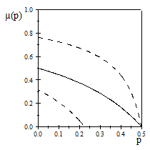
In view of (77), we can determine threshold curves $\bar{\mu}\left(p\right)$ that allow to select the two-dimensional parametric region where error correction schemes are useful. For instance, considering the model I in absence of correlations, it follows that the three-qubit code is effective only if $p<0.5$. However for such values of the error probability, the DFS considered does not work for $\mu$ approaching zero. The threshold curve for the DFS for the model I appear in Figure $1$. The DFS works only in the parametric region above the thin solid line in Figure 1, while the three-qubit bit-flip code works for all values of the memory degree $\mu$ when the error probability is less than $0.5$.

III.2.2 Model II

We consider $\Lambda_{\mu}^{\left(n\right)}\left(\rho\right)$ in (19) with $n=2$. Technical details will be omitted. They can be obtained by following the line of reasoning presented when studying the error avoiding code applied to the model I. It turns out that,

β„±D​F​S(2)​(μ​, ​p)=μ​(βˆ’2​p2+2​p)+(2​p2βˆ’2​p+1)​ (model II).superscriptsubscriptℱ𝐷𝐹𝑆2πœ‡,Β π‘πœ‡2superscript𝑝22𝑝2superscript𝑝22𝑝1Β (model II).\mathcal{F}_{DFS}^{\left(2\right)}\left(\mu\text{, }p\right)=\mu\left(-2p^{2}+2p\right)+\left(2p^{2}-2p+1\right)\text{ (model II).} (78)

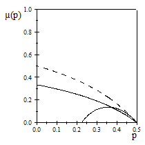
Notice that the entanglement fidelities in (76) and (78) are equal. Finally, the threshold curves for the three-qubit bit flip and DFS for the model II appear in Figure $2$. The DFS works only in the parametric region above the dashed line while the three-qubit code works only below the thin solid line.

Refer to caption
Figure 2: Threshold curves for model II: DFS (dashed line), three-qubit bit flip code (thin solid line), concatenated code (thick solid line).

IV Concatenated Codes

IV.1 Model I

Error Operators. Consider the limiting case of (16) with $n=6$ qubits and correlated errors in a bit flip quantum channel,

$$\Lambda^{(6)}(\rho)\overset{\text{def}}{=}\sum_{i_{1}\text{,..., }i_{6}=0}^{1}p_{i_{6}|i_{5}}p_{i_{5}|i_{4}}p_{i_{4}|i_{3}}p_{i_{3}|i_{2}}p_{i_{2}|i_{1}}p_{i_{1}}\left(A_{i_{6}}A_{i_{5}}A_{i_{4}}A_{i_{3}}A_{i_{2}}A_{i_{1}}\right)\rho\left(A_{i_{6}}A_{i_{5}}A_{i_{4}}A_{i_{3}}A_{i_{2}}A_{i_{1}}\right)^{\dagger}\text{,}$$ (79)

The error superoperator $\mathcal{A}$ associated to channel (79) is defined in terms of the following error operators,

π’œβŸ·{A0′​,.., ​A63β€²}​ with ​Λ(6)​(ρ)​=defβ€‹βˆ‘k=026βˆ’1Ak′​ρ​Ak′⁣†​ and,Β β€‹βˆ‘k=026βˆ’1Ak′⁣†​Akβ€²=I64Γ—64​.βŸ·π’œsuperscriptsubscript𝐴0β€²,..,Β superscriptsubscript𝐴63β€²Β withΒ superscriptΞ›6𝜌defsuperscriptsubscriptπ‘˜0superscript261superscriptsubscriptπ΄π‘˜β€²πœŒsuperscriptsubscriptπ΄π‘˜β€²β€ Β and,Β superscriptsubscriptπ‘˜0superscript261superscriptsubscriptπ΄π‘˜β€²β€ superscriptsubscriptπ΄π‘˜β€²subscript𝐼6464.\mathcal{A}\longleftrightarrow\left\{A_{0}^{\prime}\text{,.., }A_{63}^{\prime}\right\}\text{ with }\Lambda^{(6)}(\rho)\overset{\text{def}}{=}\sum\limits_{k=0}^{2^{6}-1}A_{k}^{\prime}\rho A_{k}^{\prime\dagger}\text{ and, }\sum\limits_{k=0}^{2^{6}-1}A_{k}^{\prime\dagger}A_{k}^{\prime}=I_{64\times 64}\text{.} (80)

The error operators in the Kraus decomposition (80) are $2^{6}=64$,

$$\sum_{k=0}^{6}\binom{6}{k}=2^{6}\text{,}$$ (81)

where $\binom{6}{k}$ is the cardinality of weight-$k$ error operators.

Encoding Operator. We encode our logical qubit with a concatenated subspace obtained by combining the decoherence free subspace in (63) (inner code, $\mathcal{C}_{DFS}=\mathcal{C}_{\text{inner}}$ ) with the three-qubit bit flip code in (26) (outer code, $\mathcal{C}_{\text{bit}}=\mathcal{C}_{\text{outer}}$). We obtain that the codewords of the concatenated code $\mathcal{C}=\mathcal{C}_{DFS}\circ\mathcal{C}_{\text{bit}}$ are given by,

$\displaystyle\left|0_{L}\right\rangle$ $\displaystyle=$ $\displaystyle\frac{1}{2}\left(\left|000000\right\rangle-\left|000111\right\rangle+\left|111000\right\rangle-\left|111111\right\rangle\right)\text{,}$
$\displaystyle\left|1_{L}\right\rangle$ $\displaystyle=$ $\displaystyle\frac{1}{2}\left(\left|000000\right\rangle+\left|000111\right\rangle-\left|111000\right\rangle-\left|111111\right\rangle\right)\text{.}$ (82)

As a side remark, we point out that a suitable concatenated code for the case of a phase flip Markovian correlated noise model is given by $\left|0\right\rangle\longrightarrow\left|0_{L}\right\rangle=\left|+++---\right\rangle$ and, $\left|1\right\rangle\longrightarrow\left|1_{L}\right\rangle=\left|---+++\right\rangle$.

Correctable Errors and Recovery Operators. Recall that the detectability condition is given by $P_{\mathcal{C}}A_{k}^{\prime}P_{\mathcal{C}}=\lambda_{A_{k}^{\prime}}P_{\mathcal{C}}$ where the projector operator on the code space $\mathcal{C}$ is $P_{\mathcal{C}}=\left|0_{L}\right\rangle\left\langle 0_{L}\right|+\left|1_{L}\right\rangle\left\langle 1_{L}\right|$. Observe that,

$$P_{\mathcal{C}}A_{k}^{\prime}P_{\mathcal{C}}=\left\langle 0_{L}|A_{k}^{\prime}|0_{L}\right\rangle\left|0_{L}\right\rangle\left\langle 0_{L}\right|+\left\langle 0_{L}|A_{k}^{\prime}|1_{L}\right\rangle\left|0_{L}\right\rangle\left\langle 1_{L}\right|+\left\langle 1_{L}|A_{k}^{\prime}|0_{L}\right\rangle\left|1_{L}\right\rangle\left\langle 0_{L}\right|+\left\langle 1_{L}|A_{k}^{\prime}|1_{L}\right\rangle\left|1_{L}\right\rangle\left\langle 1_{L}\right|\text{.}$$ (83)

Therefore, it turns out that for detectable error operators we must have,

$$\left\langle 0_{L}|A_{k}^{\prime}|0_{L}\right\rangle=\left\langle 1_{L}|A_{k}^{\prime}|1_{L}\right\rangle\text{ and, }\left\langle 0_{L}|A_{k}^{\prime}|1_{L}\right\rangle=\left\langle 1_{L}|A_{k}^{\prime}|0_{L}\right\rangle=0\text{.}$$ (84)

In the case under consideration, it follows that the only error operators (omitting for the sake of simplicity the proper error amplitudes) not fulfilling the above conditions are proportional to,

$$X^{1}X^{2}X^{3}\text{ and }X^{4}X^{5}X^{6}\text{.}$$ (85)

For such operators, we get

⟨0L|X1​X2​X3|0L⟩=1​,Β β€‹βŸ¨1L|X1​X2​X3|1L⟩=βˆ’1​, and,Β β€‹βŸ¨0L|X4​X5​X6|0L⟩=βˆ’1​,Β β€‹βŸ¨1L|X4​X5​X6|1L⟩=1​.quantum-operator-productsubscript0𝐿superscript𝑋1superscript𝑋2superscript𝑋3subscript0𝐿1,Β quantum-operator-productsubscript1𝐿superscript𝑋1superscript𝑋2superscript𝑋3subscript1𝐿1, and,Β quantum-operator-productsubscript0𝐿superscript𝑋4superscript𝑋5superscript𝑋6subscript0𝐿1,Β quantum-operator-productsubscript1𝐿superscript𝑋4superscript𝑋5superscript𝑋6subscript1𝐿1.\left\langle 0_{L}|X^{1}X^{2}X^{3}|0_{L}\right\rangle=1\text{, }\left\langle 1_{L}|X^{1}X^{2}X^{3}|1_{L}\right\rangle=-1\text{, and, }\left\langle 0_{L}|X^{4}X^{5}X^{6}|0_{L}\right\rangle=-1\text{, }\left\langle 1_{L}|X^{4}X^{5}X^{6}|1_{L}\right\rangle=1\text{.} (86)

Therefore $X^{1}X^{2}X^{3}$ and $X^{4}X^{5}X^{6}$ are not detectable. Thus, the cardinality of the set of detectable errors $\mathcal{A}_{\text{detectable}}$ is $62$. Furthermore, recall that the set of correctable errors $\mathcal{A}_{\text{correctable}}$ is such that π’œcorrectableβ€ β€‹π’œcorrectablesuperscriptsubscriptπ’œcorrectable†subscriptπ’œcorrectable\mathcal{A}_{\text{correctable}}^{\dagger}\mathcal{A}_{\text{correctable}} is detectable (in the hypothesis of invertible error operators). Therefore, after some reasoning, we conclude that the set of correctable errors is composed by $32$ error operators. The correctable weight-00, $1$ and $2$ correctable error operators are (omitting the proper error amplitudes),

{I}weight-​0​, ​{X1​, ​X2​, ​X3​, ​X4​, ​X5​, ​X6}weight-​1​,Β subscript𝐼weight-0,Β subscriptsuperscript𝑋1,Β superscript𝑋2,Β superscript𝑋3,Β superscript𝑋4,Β superscript𝑋5,Β superscript𝑋6weight-1,Β \left\{I\right\}_{\text{weight-}0}\text{, }\left\{X^{1}\text{, }X^{2}\text{, }X^{3}\text{, }X^{4}\text{, }X^{5}\text{, }X^{6}\right\}_{\text{weight-}1}\text{, } (87)

and,

{X1​X4​, ​X1​X5​, ​X1​X6​, ​X2​X4​, ​X2​X5​, ​X2​X6​, ​X3​X4​, ​X3​X5​, ​X3​X6}weight-​2​,subscriptsuperscript𝑋1superscript𝑋4,Β superscript𝑋1superscript𝑋5,Β superscript𝑋1superscript𝑋6,Β superscript𝑋2superscript𝑋4,Β superscript𝑋2superscript𝑋5,Β superscript𝑋2superscript𝑋6,Β superscript𝑋3superscript𝑋4,Β superscript𝑋3superscript𝑋5,Β superscript𝑋3superscript𝑋6weight-2,\left\{X^{1}X^{4}\text{, }X^{1}X^{5}\text{, }X^{1}X^{6}\text{, }X^{2}X^{4}\text{, }X^{2}X^{5}\text{, }X^{2}X^{6}\text{, }X^{3}X^{4}\text{, }X^{3}X^{5}\text{, }X^{3}X^{6}\right\}_{\text{weight-}2}\text{,} (88)

respectively. The correctable weight-$4$ errors are,

{X1​X2​X4​X5​, ​X1​X2​X4​X6​, ​X1​X2​X5​X6​, ​X1​X3​X4​X5​, ​X1​X3​X4​X6​,Β X1​X3​X5​X6​, ​X2​X3​X4​X5​, ​X2​X3​X4​X6​, ​X2​X3​X5​X6}weight-​4​.subscriptsuperscript𝑋1superscript𝑋2superscript𝑋4superscript𝑋5,Β superscript𝑋1superscript𝑋2superscript𝑋4superscript𝑋6,Β superscript𝑋1superscript𝑋2superscript𝑋5superscript𝑋6,Β superscript𝑋1superscript𝑋3superscript𝑋4superscript𝑋5,Β superscript𝑋1superscript𝑋3superscript𝑋4superscript𝑋6,Β missing-subexpressionsuperscript𝑋1superscript𝑋3superscript𝑋5superscript𝑋6,Β superscript𝑋2superscript𝑋3superscript𝑋4superscript𝑋5,Β superscript𝑋2superscript𝑋3superscript𝑋4superscript𝑋6,Β superscript𝑋2superscript𝑋3superscript𝑋5superscript𝑋6weight-4.\left\{\begin{array}[]{c}X^{1}X^{2}X^{4}X^{5}\text{, }X^{1}X^{2}X^{4}X^{6}\text{, }X^{1}X^{2}X^{5}X^{6}\text{, }X^{1}X^{3}X^{4}X^{5}\text{, }X^{1}X^{3}X^{4}X^{6}\text{, }\\ \\ X^{1}X^{3}X^{5}X^{6}\text{, }X^{2}X^{3}X^{4}X^{5}\text{, }X^{2}X^{3}X^{4}X^{6}\text{, }X^{2}X^{3}X^{5}X^{6}\end{array}\right\}_{\text{weight-}4}\text{.} (89)

Finally, weight-$5$ and weight-$6$ error operators are given by,

{X1​X2​X3​X4​X5​, ​X1​X2​X3​X4​X6​, ​X1​X2​X4​X5​X6​, ​X1​X3​X4​X5​X6​, ​X1​X2​X3​X5​X6​, ​X2​X3​X4​X5​X6​ }weight-​5​,subscriptsuperscript𝑋1superscript𝑋2superscript𝑋3superscript𝑋4superscript𝑋5,Β superscript𝑋1superscript𝑋2superscript𝑋3superscript𝑋4superscript𝑋6,Β superscript𝑋1superscript𝑋2superscript𝑋4superscript𝑋5superscript𝑋6,Β superscript𝑋1superscript𝑋3superscript𝑋4superscript𝑋5superscript𝑋6,Β superscript𝑋1superscript𝑋2superscript𝑋3superscript𝑋5superscript𝑋6,Β superscript𝑋2superscript𝑋3superscript𝑋4superscript𝑋5superscript𝑋6Β weight-5,\left\{X^{1}X^{2}X^{3}X^{4}X^{5}\text{, }X^{1}X^{2}X^{3}X^{4}X^{6}\text{, }X^{1}X^{2}X^{4}X^{5}X^{6}\text{, }X^{1}X^{3}X^{4}X^{5}X^{6}\text{, }X^{1}X^{2}X^{3}X^{5}X^{6}\text{, }X^{2}X^{3}X^{4}X^{5}X^{6}\text{ }\right\}_{\text{weight-}5}\text{,} (90)

and,

$$\left\{X^{1}X^{2}X^{3}X^{4}X^{5}X^{6}\right\}_{\text{weight-}6}\text{,}$$ (91)

respectively. The action of the correctable errors on the codewords in (82) is such that the Hilbert space $\mathcal{H}_{2}^{6}$ can be decomposed in two $32$-dimensional orthogonal subspaces $\mathcal{V}^{0_{L}}$ and $\mathcal{V}^{1_{L}}$. In other words, $\mathcal{H}_{2}^{6}=\mathcal{V}^{0_{L}}\oplus\mathcal{V}^{1_{L}}$ where

$$\mathcal{V}^{0_{L}}=Span\left\{\left|v_{k+1}^{0_{L}}\right\rangle=\frac{1}{\sqrt{\tilde{p}_{k}^{\left(6\right)}}}A_{k}^{\prime}\left|0_{L}\right\rangle\right\}\text{ and, }\mathcal{V}^{1_{L}}=Span\left\{\left|v_{k+1}^{1_{L}}\right\rangle=\frac{1}{\sqrt{\tilde{p}_{k}^{\left(6\right)}}}A_{k}^{\prime}\left|1_{L}\right\rangle\right\}\text{,}$$ (92)

with Akβ€²βˆˆπ’œcorrectablesuperscriptsubscriptπ΄π‘˜β€²subscriptπ’œcorrectableA_{k}^{\prime}\in\mathcal{A}_{\text{correctable}} βˆ€k=0for-allπ‘˜0\forall k=0,…, 313131 (numbering the correctable error operators from 00 to 313131). Notice that ⟨vkiL|vkβ€²jL⟩=Ξ΄k​k′​δi​jinner-productsuperscriptsubscriptπ‘£π‘˜subscript𝑖𝐿superscriptsubscript𝑣superscriptπ‘˜β€²subscript𝑗𝐿subscriptπ›Ώπ‘˜superscriptπ‘˜β€²subscript𝛿𝑖𝑗\left\langle v_{k}^{i_{L}}|v_{k^{\prime}}^{j_{L}}\right\rangle=\delta_{kk^{\prime}}\delta_{ij}, with kπ‘˜k, kβ€²βˆˆ{0​,…, ​31}superscriptπ‘˜β€²0,…,Β 31k^{\prime}\in\left\{0\text{,..., }31\right\} and i𝑖i, j∈{0​, ​1}𝑗0,Β 1j\in\left\{0\text{, }1\right\} since,

⟨vkiL|vkβ€²jL⟩=⟨iL|Akβˆ’1′⁣†p~k(6)​Akβ€²βˆ’1β€²p~kβ€²(6)|jL⟩=1p~k(6)​p~kβ€²(6)β€‹βŸ¨iL|Ak′⁣†​Akβ€²β€²|jL⟩=1p~k(6)​p~kβ€²(6)​αk​k′′​δi​j=Ξ΄k​k′​δi​j​,inner-productsuperscriptsubscriptπ‘£π‘˜subscript𝑖𝐿superscriptsubscript𝑣superscriptπ‘˜β€²subscript𝑗𝐿quantum-operator-productsubscript𝑖𝐿superscriptsubscriptπ΄π‘˜1′†superscriptsubscript~π‘π‘˜6superscriptsubscript𝐴superscriptπ‘˜β€²1β€²superscriptsubscript~𝑝superscriptπ‘˜β€²6subscript𝑗𝐿1superscriptsubscript~π‘π‘˜6superscriptsubscript~𝑝superscriptπ‘˜β€²6quantum-operator-productsubscript𝑖𝐿superscriptsubscriptπ΄π‘˜β€²β€ superscriptsubscript𝐴superscriptπ‘˜β€²β€²subscript𝑗𝐿1superscriptsubscript~π‘π‘˜6superscriptsubscript~𝑝superscriptπ‘˜β€²6superscriptsubscriptπ›Όπ‘˜superscriptπ‘˜β€²β€²subscript𝛿𝑖𝑗subscriptπ›Ώπ‘˜superscriptπ‘˜β€²subscript𝛿𝑖𝑗,\left\langle v_{k}^{i_{L}}|v_{k^{\prime}}^{j_{L}}\right\rangle=\left\langle i_{L}|\frac{A_{k-1}^{\prime\dagger}}{\sqrt{\tilde{p}_{k}^{\left(6\right)}}}\frac{A_{k^{\prime}-1}^{\prime}}{\sqrt{\tilde{p}_{k^{\prime}}^{\left(6\right)}}}|j_{L}\right\rangle=\frac{1}{\sqrt{\tilde{p}_{k}^{\left(6\right)}\tilde{p}_{k^{\prime}}^{\left(6\right)}}}\left\langle i_{L}|A_{k}^{\prime\dagger}A_{k^{\prime}}^{\prime}|j_{L}\right\rangle=\frac{1}{\sqrt{\tilde{p}_{k}^{\left(6\right)}\tilde{p}_{k^{\prime}}^{\left(6\right)}}}\alpha_{kk^{\prime}}^{\prime}\delta_{ij}=\delta_{kk^{\prime}}\delta_{ij}\text{,} (93)

where we have used the fact that the square (Hermitian) matrix $\alpha_{kk^{\prime}}^{\prime}$ equals $\sqrt{\tilde{p}_{k}^{\left(6\right)}\tilde{p}_{k^{\prime}}^{\left(6\right)}}$ $\delta_{kk^{\prime}}$. The recovery superoperator $\mathcal{R}\leftrightarrow\left\{R_{l}\right\}$ with $l=1$,.., $32$ is defined as knill97 ,

$$R_{l}\overset{\text{def}}{=}V_{l}\sum_{i=0}^{1}\left|v_{l}^{i_{L}}\right\rangle\left\langle v_{l}^{i_{L}}\right|\text{,}$$ (94)

where the unitary operator Vlsubscript𝑉𝑙V_{l} is such that Vl​|vliL⟩=|iL⟩subscript𝑉𝑙ketsuperscriptsubscript𝑣𝑙subscript𝑖𝐿ketsubscript𝑖𝐿V_{l}\left|v_{l}^{i_{L}}\right\rangle=\left|i_{L}\right\rangle for i∈{0​, ​1}𝑖0,Β 1i\in\left\{0\text{, }1\right\}. Notice that,

$$R_{l}\overset{\text{def}}{=}V_{l}\sum_{i=0}^{1}\left|v_{l}^{i_{L}}\right\rangle\left\langle v_{l}^{i_{L}}\right|=\left|0_{L}\right\rangle\left\langle v_{l}^{0_{L}}\right|+\left|1_{L}\right\rangle\left\langle v_{l}^{1_{L}}\right|\text{.}$$ (95)

If turns out that the $32$ recovery operators are given by,

$$R_{l+1}=R_{1}\frac{A_{l}^{\prime}}{\sqrt{\tilde{p}_{l}^{\prime}}}=\left(\left|0_{L}\right\rangle\left\langle 0_{L}\right|+\left|1_{L}\right\rangle\left\langle 1_{L}\right|\right)\frac{A_{l}^{\prime}}{\sqrt{\tilde{p}_{l}^{\prime}}}\text{,}$$ (96)

with $l\in\left\{0\text{,..., }31\right\}$. Notice that $\mathcal{R}\leftrightarrow\left\{R_{l}\right\}$ is a trace preserving quantum operation since,

βˆ‘l=132Rl†​Rl=βˆ‘l=132(βˆ‘iL|iLβŸ©β€‹βŸ¨vliL|)†​(βˆ‘jL|jLβŸ©β€‹βŸ¨vljL|)=βˆ‘l=132βˆ‘iL​, ​jL|vliLβŸ©β€‹βŸ¨iL|jLβŸ©β€‹βŸ¨vljL|=βˆ‘l=132βˆ‘iL|vliLβŸ©β€‹βŸ¨vliL|=I64Γ—64​,superscriptsubscript𝑙132superscriptsubscript𝑅𝑙†subscript𝑅𝑙superscriptsubscript𝑙132superscriptsubscriptsubscript𝑖𝐿ketsubscript𝑖𝐿brasuperscriptsubscript𝑣𝑙subscript𝑖𝐿†subscriptsubscript𝑗𝐿ketsubscript𝑗𝐿brasuperscriptsubscript𝑣𝑙subscript𝑗𝐿superscriptsubscript𝑙132subscriptsubscript𝑖𝐿,Β subscript𝑗𝐿ketsuperscriptsubscript𝑣𝑙subscript𝑖𝐿inner-productsubscript𝑖𝐿subscript𝑗𝐿brasuperscriptsubscript𝑣𝑙subscript𝑗𝐿superscriptsubscript𝑙132subscriptsubscript𝑖𝐿ketsuperscriptsubscript𝑣𝑙subscript𝑖𝐿brasuperscriptsubscript𝑣𝑙subscript𝑖𝐿subscript𝐼6464,\sum_{l=1}^{32}R_{l}^{\dagger}R_{l}=\sum_{l=1}^{32}\left(\sum_{i_{L}}\left|i_{L}\right\rangle\left\langle v_{l}^{i_{L}}\right|\right)^{\dagger}\left(\sum_{j_{L}}\left|j_{L}\right\rangle\left\langle v_{l}^{j_{L}}\right|\right)=\sum_{l=1}^{32}\sum_{i_{L\text{, }}j_{L}}\left|v_{l}^{i_{L}}\right\rangle\left\langle i_{L}|j_{L}\right\rangle\left\langle v_{l}^{j_{L}}\right|=\sum_{l=1}^{32}\sum_{i_{L}}\left|v_{l}^{i_{L}}\right\rangle\left\langle v_{l}^{i_{L}}\right|=I_{64\times 64}\text{,} (97)

since {|vliL⟩}ketsuperscriptsubscript𝑣𝑙subscript𝑖𝐿\left\{\left|v_{l}^{i_{L}}\right\rangle\right\} with l=1𝑙1l=1,…, 323232 and iL∈{0​, ​1}subscript𝑖𝐿0,Β 1i_{L}\in\left\{0\text{, }1\right\} is an orthonormal basis for β„‹26superscriptsubscriptβ„‹26\mathcal{H}_{2}^{6}. Finally, the action of this recovery operation β„›β„›\mathcal{R} on the map Ξ›(6)​(ρ)superscriptΞ›6𝜌\Lambda^{\left(6\right)}\left(\rho\right) in (80) leads to,

Ξ›recover(6)​(ρ)≑(β„›βˆ˜Ξ›(6))​(ρ)​=defβ€‹βˆ‘k=026βˆ’1βˆ‘l=132(Rl​Akβ€²)​ρ​(Rl​Akβ€²)†​.superscriptsubscriptΞ›recover6πœŒβ„›superscriptΞ›6𝜌defsuperscriptsubscriptπ‘˜0superscript261superscriptsubscript𝑙132subscript𝑅𝑙superscriptsubscriptπ΄π‘˜β€²πœŒsuperscriptsubscript𝑅𝑙superscriptsubscriptπ΄π‘˜β€²β€ .\Lambda_{\text{recover}}^{\left(6\right)}\left(\rho\right)\equiv\left(\mathcal{R\circ}\Lambda^{(6)}\right)\left(\rho\right)\overset{\text{def}}{=}\sum_{k=0}^{2^{6}-1}\sum\limits_{l=1}^{32}\left(R_{l}A_{k}^{\prime}\right)\rho\left(R_{l}A_{k}^{\prime}\right)^{\dagger}\text{.} (98)

Entanglement Fidelity. We want to describe the action of $\mathcal{R\circ}\Lambda^{(6)}$ restricted to the code subspace $\mathcal{C}$. Recalling that $A_{l}^{\prime}=A_{l}^{\prime\dagger}$, it turns out that,

$$\left\langle i_{L}|R_{l+1}A_{k}^{\prime}|j_{L}\right\rangle=\frac{1}{\sqrt{\tilde{p}_{l}^{\prime}}}\left\langle i_{L}|0_{L}\right\rangle\left\langle 0_{L}|A_{l}^{\prime\dagger}A_{k}^{\prime}|j_{L}\right\rangle+\frac{1}{\sqrt{\tilde{p}_{l}^{\prime}}}\left\langle i_{L}|1_{L}\right\rangle\left\langle 1_{L}|A_{l}^{\prime\dagger}A_{k}^{\prime}|j_{L}\right\rangle\text{.}$$ (99)

We now need to compute the $2\times 2$ matrix representation $\left[R_{l}A_{k}^{\prime}\right]_{|\mathcal{C}}$ of each $R_{l}A_{k}^{\prime}$ with $l=0$,.., $31$ and $k=0$,.., $2^{6}-1$ where,

$$\left[R_{l+1}A_{k}^{\prime}\right]_{|\mathcal{C}}\overset{\text{def}}{=}\left(\begin{array}[]{cc}\left\langle 0_{L}|R_{l+1}A_{k}^{\prime}|0_{L}\right\rangle&\left\langle 0_{L}|R_{l+1}A_{k}^{\prime}|1_{L}\right\rangle\\ \left\langle 1_{L}|R_{l+1}A_{k}^{\prime}|0_{L}\right\rangle&\left\langle 1_{L}|R_{l+1}A_{k}^{\prime}|1_{L}\right\rangle\end{array}\right)\text{.}$$ (100)

For $l$, $k=0$,.., $31$, we note that $\left[R_{l+1}A_{k}^{\prime}\right]_{|\mathcal{C}}$ becomes,

$$\left[R_{l+1}A_{k}^{\prime}\right]_{|\mathcal{C}}=\left(\begin{array}[]{cc}\left\langle 0_{L}|A_{l}^{\prime\dagger}A_{k}^{\prime}|0_{L}\right\rangle&0\\ 0&\left\langle 1_{L}|A_{l}^{\prime\dagger}A_{k}^{\prime}|1_{L}\right\rangle\end{array}\right)=\sqrt{\tilde{p}_{l}^{\prime}}\delta_{lk}\left(\begin{array}[]{cc}1&0\\ 0&1\end{array}\right)\text{,}$$ (101)

while for any pair (l​, ​k)𝑙,Β π‘˜\left(l\text{, }k\right) with l𝑙l =0absent0=0,.., 313131 and k>31π‘˜31k>31, it follows that,

$$\left\langle 0_{L}|R_{l+1}A_{k}^{\prime}|0_{L}\right\rangle+\left\langle 1_{L}|R_{l+1}A_{k}^{\prime}|1_{L}\right\rangle=0\text{.}$$ (102)

We conclude that the only matrices $\left[R_{l}A_{k}^{\prime}\right]_{|\mathcal{C}}$ with non-vanishing trace are given by $\left[R_{l+1}A_{l}^{\prime}\right]_{|\mathcal{C}}$ with $l$ $=0$,.., $31$ where,

$$\left[R_{l+1}A_{l}^{\prime}\right]_{|\mathcal{C}}=\sqrt{\tilde{p}_{l}^{\prime}}\left(\begin{array}[]{cc}1&0\\ 0&1\end{array}\right)\text{.}$$ (103)

Therefore, the entanglement fidelity β„±conc(6)​(μ​, ​p)superscriptsubscriptβ„±conc6πœ‡, 𝑝\mathcal{F}_{\text{conc}}^{\left(6\right)}\left(\mu\text{, }p\right) defined as,

β„±conc(6)​(μ​, ​p)​=def​ℱconc(6)​(12​I2Γ—2​,Β β€‹β„›βˆ˜Ξ›(6))=1(2)2β€‹βˆ‘k=026βˆ’1βˆ‘l=132|tr​([Rl​Akβ€²]|π’ž)|2​,\mathcal{F}_{\text{conc}}^{\left(6\right)}\left(\mu\text{, }p\right)\overset{\text{def}}{=}\mathcal{F}_{\text{conc}}^{\left(6\right)}\left(\frac{1}{2}I_{2\times 2}\text{, }\mathcal{R\circ}\Lambda^{(6)}\right)=\frac{1}{\left(2\right)^{2}}\sum_{k=0}^{2^{6}-1}\sum\limits_{l=1}^{32}\left|\text{tr}\left(\left[R_{l}A_{k}^{\prime}\right]_{|\mathcal{C}}\right)\right|^{2}\text{,} (104)

becomes,

Refer to caption
Figure 3: Entanglement fidelity vs. memory parameter $\mu$ with $p=10^{-1}$ for model II: concatenated code (dashed line), DFS (thin solid line) and three-qubit bit flip code (thick solid line).
β„±conc(6)​(μ​, ​p)superscriptsubscriptβ„±conc6πœ‡, 𝑝\displaystyle\mathcal{F}_{\text{conc}}^{\left(6\right)}\left(\mu\text{, }p\right) =\displaystyle= p005​p0+2​p004​p10​p0+p003​p01​p10​(4​p0+p1)+4​p002​p01​p102​p0+p002​p01​p10​p11​p0+3​p00​p012​p102​p0+superscriptsubscript𝑝005subscript𝑝02superscriptsubscript𝑝004subscript𝑝10subscript𝑝0superscriptsubscript𝑝003subscript𝑝01subscript𝑝104subscript𝑝0subscript𝑝14superscriptsubscript𝑝002subscript𝑝01superscriptsubscript𝑝102subscript𝑝0superscriptsubscript𝑝002subscript𝑝01subscript𝑝10subscript𝑝11subscript𝑝0limit-from3subscript𝑝00superscriptsubscript𝑝012superscriptsubscript𝑝102subscript𝑝0\displaystyle p_{00}^{5}p_{0}+2p_{00}^{4}p_{10}p_{0}+p_{00}^{3}p_{01}p_{10}\left(4p_{0}+p_{1}\right)+4p_{00}^{2}p_{01}p_{10}^{2}p_{0}+p_{00}^{2}p_{01}p_{10}p_{11}p_{0}+3p_{00}p_{01}^{2}p_{10}^{2}p_{0}+ (105)
$\displaystyle+4p_{01}p_{10}^{2}p_{11}^{2}p_{0}+3p_{01}^{2}p_{10}^{2}p_{11}p_{1}+p_{00}p_{01}p_{10}p_{11}^{2}p_{1}+p_{01}p_{10}p_{11}^{3}\left(p_{0}+4p_{1}\right)+2p_{10}p_{11}^{4}p_{0}+p_{11}^{5}p_{1}\text{.}$

Substituting (25) into (105), we finally get

β„±conc(6)​(μ​, ​p)superscriptsubscriptβ„±conc6πœ‡, 𝑝\displaystyle\mathcal{F}_{\text{conc}}^{\left(6\right)}\left(\mu\text{, }p\right) =\displaystyle= ΞΌ5​(βˆ’8​p6+24​p5βˆ’24​p4+8​p3)+ΞΌ4​(40​p6βˆ’120​p5+130​p4βˆ’60​p3+10​p2)+superscriptπœ‡58superscript𝑝624superscript𝑝524superscript𝑝48superscript𝑝3limit-fromsuperscriptπœ‡440superscript𝑝6120superscript𝑝5130superscript𝑝460superscript𝑝310superscript𝑝2\displaystyle\mu^{5}\left(-8p^{6}+24p^{5}-24p^{4}+\allowbreak 8p^{3}\right)+\mu^{4}\left(40p^{6}-120p^{5}+130p^{4}\allowbreak-60p^{3}+10p^{2}\right)+ (106)
$\displaystyle+\mu^{3}\left(-80p^{6}+240p^{5}-264p^{4}+128p^{3}-26p^{2}+2p\right)+$
$\displaystyle+\mu^{2}\left(80p^{6}-\allowbreak 240p^{5}+252p^{4}-104p^{3}+10p^{2}+2p\right)+$
$\displaystyle+\mu\left(-40\allowbreak p^{6}+120p^{5}-112p^{4}+24\allowbreak p^{3}+12\allowbreak p^{2}-4p\right)+\left(8p^{6}-24p^{5}+18p^{4}+4p^{3}-6p^{2}+1\right)\text{.}$

The threshold curves for the concatenated code defined in (82) for the model I appear in Figure $1$. It turns out that the concatenated code does not work in the region delimited by the two dashed lines. We emphasize that in view of equations (52), (76) and (106), it turns out that the concatenated code outperforms the bit-flip code in regions with very high memory parameter values and outperforms the DFS in regions with low memory parameter values. In particular,Β the relevance of the concatenation trick shines where the weaknesses of the inner and outer codes (yet not concatenated) are more pronounced, that is in regions with both high error probability and low memory parameter values. It is within this area that we can identify the region where the concatenated code outperforms both the inner and the outer codes. However, there is a big parametric region characterized by intermediate values of the degree of memory Β (see Figure I) where the concatenation trick does not work well for model I. On the contrary, we will show that the quantum coding trick is particularly useful for the model II in the presence of partial correlations.

IV.2 Model II

We consider $\Lambda_{\mu}^{\left(n\right)}\left(\rho\right)$ in (19) with $n=6$. Technical details will be omitted. They can be obtained by following the line of reasoning presented when studying the concatenated code applied to the model I. It turns out that,

β„±conc(6)​(μ​, ​p)=μ​(βˆ’8​p6+24​p5βˆ’18​p4βˆ’4​p3+6​p2)+(8​p6βˆ’24​p5+18​p4+4​p3βˆ’6​p2+1)​.superscriptsubscriptβ„±conc6πœ‡,Β π‘πœ‡8superscript𝑝624superscript𝑝518superscript𝑝44superscript𝑝36superscript𝑝28superscript𝑝624superscript𝑝518superscript𝑝44superscript𝑝36superscript𝑝21.\mathcal{F}_{\text{conc}}^{\left(6\right)}(\mu\text{, }p)=\mu\left(-8p^{6}+24p^{5}-18p^{4}-4p^{3}+6p^{2}\right)+\left(8p^{6}-24p^{5}+18p^{4}+4p^{3}-6p^{2}+1\right)\text{.} (107)

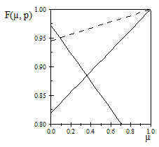
The threshold curve for the concatenated code defined in (82) for the model II appears in Figure 222. It follows that while none of the two codes is effective in the extreme limit when the other is, the three-qubit bit flip (phase flip) code still works for correlated errors, whereas the error avoiding code does not work in the absence of correlations. The concatenated code works everywhere except below the thick solid curve in Figure 222. Here there is a parametric region characterized by partial correlations and delimited by the dashed and thin solid lines where only the concatenated code is effective. Furthermore, from (58), (78) and (107), it follows that the concatenated code is especially advantageous for the model II for partially correlated error operators. For the sake of clarity, in Figure 333 we plot the entanglement fidelities (78) (thin solid line), (107) (dashed line) and (58) (tick solid line) for p=10βˆ’1𝑝superscript101p=10^{-1}. For such value of the error probability, the error avoiding code only works for μ≳0.44greater-than-or-equivalent-toπœ‡0.44\mu\gtrsim 0.44 (threshold value obtained from Figure 222), the three-qubit bit flip code only works for μ≲0.30less-than-or-similar-toπœ‡0.30\mu\lesssim 0.30 (threshold value obtained from Figure 222) while the concatenated code with entanglement fidelity given in (107) is is efficient for any value of μ∈[0​, ​1]πœ‡delimited-[]0,Β 1\mu\in\left[0\text{, }1\right].

V Final Remarks

In this article, we studied the performance of simple error correcting and error avoiding quantum codes together with their concatenation for correlated noise models. For model I, a bit-flip (phase-flip) noisy Markovian memory channel, we have applied both the three-qubit bit flip (phase flip) and a suitable error avoiding code. The performance of the codes was quantified in terms of the entanglement fidelities in (52) and (76). The performance of the concatenated code applied to model I appears in (106). In Figure $1$, we have plotted the parametric regions where error correction is effective. We have presented a similar analysis for the model II, a memory channel defined as a memory degree dependent linear combination of memoryless channels with Kraus decompositions expressed solely in terms of tensor products of $X$-Pauli ($Z$-Pauli) operators (model II). The performance of the codes was quantified in terms of the entanglement fidelities in (58) and (78). The performance of the concatenated code applied to model II appears in (107). In Figure $2$, we have plotted the parametric regions where error correction schemes are effective.

Our analysis explicitly shows that while none of the two codes is effective in the extreme limit when the other is, the three-qubit bit flip (phase flip) code still works for correlated errors, whereas the error avoiding code does not work in the absence of correlations. Finally, our final finding leads to conclude that the concatenated code in (82) is particularly advantageous for model II in the regime of partial correlations (see Figure $3$).

Acknowledgements.
C. C. thanks S. L’Innocente and C. Lupo for useful discussions. This work was supported by the European Community’s Seventh Framework Program under grant agreement 213681 (CORNER Project; FP7/2007-2013).

References

  • (1) D. Gottesman, ”An Introduction to Quantum Error Correction and Fault-Tolerant Quantum Computation”, arXiv:quant-ph/0904.2557 (2009).
  • (2) D. A. Lidar and K. B. Whaley, ”Decoherence-Free Subspaces and Subsystems”, arXiv:quant-ph/0301032 (2003).
  • (3) A. Garg, ”Decoherence in Ion Trap Quantum Computers”, Phys. Rev. Lett. 77, 964 (1996).
  • (4) D. Loss and D. P. Di Vincenzo, ”Quantum computation with quantum dots”, Phys. Rev. A57, 120 (1998).
  • (5) W. Y. Hwang et al., ”Correlated errors in quantum-error corrections”, Phys. Rev. A63, 022303 (2001).
  • (6) J. P. Clemens et al., ”Quantum error correction against correlated noise”, Phys. Rev. A69, 062313 (2004).
  • (7) R. Klesse and S. Frank, ”Quantum Error Correction in Spatially Correlated Quantum Noise”, Phys. Rev. Lett. 95, 230503 (2005).
  • (8) A. Shabani, ”Correlated errors can lead to better performance of quantum codes”, Phys. Rev. A77, 022323 (2008).
  • (9) A. D’Arrigo et al., ”Memory effects in a Markovian chain dephasing channel”, Int. J. Quantum Inf. 6, 651 (2008).
  • (10) C. Cafaro and S. Mancini, ”Repetition Versus Noiseless Quantum Codes For Correlated Errors”, Phys. Lett. A374, 2688 (2010).
  • (11) D. Gottesman, ”Pasting quantum codes”, arXiv:quant-ph/9607027 (1996).
  • (12) R. A. Calderbank et al., ”Quantum error correction via codes over $GF(4)$”, IEEE Trans. Inf. Theor. 44, 1369 (1998).
  • (13) G. D. Forley, Jr., ”Concatenated Codes”, MIT Press (1966).
  • (14) D. Gottesman, ”Stabilizer codes and quantum error correction”, PhD Thesis, Caltech (1997).
  • (15) E. Knill and R. Laflamme, ”Concatenated Quantum Codes”, arXiv:quant-ph/9608012 (1996).
  • (16) D. A. Lidar et al., ”Concatenating Decoherence-Free Subspaces with Quantum Error Correcting Codes”, Phys. Rev. Lett. 82, 4556 (1999).
  • (17) D. Gottesman, ”Class of quantum error-correcting codes saturating the quantum Hamming bound”, Phys. Rev. A54, 1862 (1996).
  • (18) E. Knill and R. Laflamme, ”Theory of quantum error-correcting codes”, Phys. Rev. A55, 900 (1997).
  • (19) D. A. Lidar et al., ”Decoherence-Free Subspaces for Quantum Computation”, Phys. Rev. Lett. 81, 2594 (1998).
  • (20) F. Gaitan, ”Quantum Error Correction and Fault Tolerant Quantum Computing”, CRC Press (2008).
  • (21) B. Schumacher, ”Sending entanglement through noisy quantum channels”, Phys. Rev. A54, 2615 (1996).
  • (22) M. A. Nielsen, ”The entanglemet fidelity and quantum error correction”, arXiv: quant-ph/9606012 (1996).
  • (23) E. Knill et al., ”Introduction to Quantum Error Correction”, arXiv:quant-ph/020717 (2002).
  • (24) M.Β A. Nielsen and I. L. Chuang, ”Quantum Computation and Information”, Cambridge University Press (2000).