Abstract

We propose a new lattice superfield formalism in momentum representation which accommodates species doublers of the lattice fermions and their bosonic counterparts as super multiplets. We explicitly show that one dimensional $N=2$ model with interactions has exact Lie algebraic supersymmetry on the lattice for all super charges.

In coordinate representation the finite difference operator is made to satisfy Leibnitz rule by introducing a non local product, the “star” product, and the exact lattice supersymmetry is realized. The standard momentum conservation is replaced on the lattice by the conservation of the sine of the momentum, which plays a crucial role in the formulation. Half lattice spacing structure is essential for the one dimensional model and the lattice supersymmetry transformation can be identified as a half lattice spacing translation combined with alternating sign structure. Invariance under finite translations and locality in the continuum limit are explicitly investigated and shown to be recovered. Supersymmetric Ward identities are shown to be satisfied at one loop level. Lie algebraic lattice supersymmetry algebra of this model suggests a close connection with Hopf algebraic exactness of the link approach formulation of lattice supersymmetry.

PACS codes: 11.15.Ha, 11.30.Pb, 11.10.Kk.

Keywords: lattice supersymmetry, lattice field theory.

1 Introduction

If we regularize massless fermions naively on a lattice, it is unavoidable that species doublers appear. Since massless particles cannot be put in the rest frame by means of a Lorentz transformation, helicity or chirality cannot be changed with a momentum change, while species doublers in different momentum region may have different helicity. Therefore species doublers have to be considered as different particles [1]. However, species doublers of chiral fermions on a lattice are usually considered as unwanted particles, the so called doubling problem, although the enlarged degree of freedom (d.o.f.) is customarily identified as a flavor (taste) d.o.f..

The equivalence of the above naive fermion formulation and the staggered fermion formulation can be shown by a spin diagonalization procedure [2] and the staggered fermion can be transformed into the Kogut-Susskind type fermion formulation [3] by considering double size lattice structure, where the flavor d.o.f. was identified [4]. This double size structure makes it possible to have a correspondence with differential forms and then the equivalence of the staggered fermion and Dirac-Kähler fermion on the lattice can be proved by introducing a noncommutativity between differential forms and fields [5]. Therefore all these lattice fermion formulations are exactly equivalent.

In the link approach of lattice supersymmetry [6], the super charges are expanded on the basis of Dirac matrices by the Dirac-Kähler twisting procedure [7]. The corresponding d.o.f. of the super charges are then exactly the same as those of fermionic species doublers and the geometric correspondence between the particles as species doublers and super multiplets is expected from the equivalence of the naive fermion and Dirac-Kähler fermion formulations on the lattice. In other words the species doublers are necessary fields to construct the super multiplets of extended supersymmetry: $N=2$ in two dimensions and N=4 in four dimensions. The flavor (taste) d.o.f. of chiral fermions are thus expected to be identified as extended supersymmetry d.o.f.. In this paper we explicitly show how the species doublers for both fermions and bosons can be identified as super multiplets of extended supersymmetry for the simplest model of $N=2$ in one dimension. We propose to introduce lattice counter parts of bosonic and fermionic “superfields” where species doublers are accommodated.

The one dimensional $N=2$ model was proposed as a supersymmetric quantum mechanics by Witten [8] and the lattice version has been investigated by several authors [9, 10] as the simplest model to clarify the fundamental problems of lattice supersymmetry. It was shown that a species doubler of the Wilson fermion term, having a mass proportional to the inverse lattice constant, breaks supersymmetry and a bosonic counter term is needed to remove the unwanted contribution [10]. Numerical evaluation of boson and fermion masses show that they approach the same value in the continuum limit, suggesting the recovery of supersymmetry, only when the counter term is introduced [9, 11]. In this model the species doubler interferes with supersymmetry and its influence has to be removed by the bosonic counter term. It has also been recognized that only one exact supersymmetry of the type $Q^{2}=0$, which can be identified as the scalar part of a twisted supersymmetry for this supersymmetric quantum mechanics, is realized when interaction terms are included [11]. This system also provides a nice arena for a numerical method for detecting spontaneous supersymmetry breaking [12].

One dimensional $N=2$ lattice supersymmetric model of this paper is constructed in parallel to the continuum superspace formulation [13, 14, 15] and is slightly different from the supersymmetric quantum mechanics model. The lattice model we propose in this paper is exactly supersymmetric for two supersymmetry charges even with interaction terms and the counter term is not necessary to fulfill Ward-Takahshi identity since the bosonic and fermionic species doublers are identified as physical particles in supermultiplets. In the momentum representation this model has, however, a lattice counter part of trigonometric momentum conservation, which was first proposed by Dondi and Nicolai [16] in the very first paper of lattice supersymmetry. In the coordinate space we introduce a new star product which makes the lattice difference operator satisfy Leibniz rule and then the exact lattice supersymmetry is realized. The model has mildly nonlocal interactions which approach local interactions in the continuum limit.

There is a long history of attempts to realize exact sypersymmetry on a lattice. See [11, 17] for some references. However exact lattice supersymmetry with interactions for full extended supersymmetry has never been realized except for the nilpotent super charge. This difficulty is essentially related to the lattice chiral fermion problem and to the breakdown of the Leibniz rule for the lattice difference operator. Instead of formulating an exact supersymmetry for local interactions in the coordinate space, there has been several attempts that approach the problem from momentum representation point of view [18, 19, 20]. This may be related to the following claim: if one tries to include the difference operator in a supersymmetry algebra, one cannot avoid introducing nonlocal interactions [21]. The momentum representation can take care the nonlocal nature of the formulation. In this paper we first establish a formulation of exact lattice supersymmetry in the momentum representation. Then we reformulate the momentum space version into the coordinate space by introducing a new non local “star” product.

In the link approach for lattice supersymmetry [6] the claim that exact lattice supersymmetry had been realized for all super charges was questioned by several authors [14, 22]. In fact it was stressed that all the extended supersymmetry are broken when the shift parameter of the scalar super charge is non zero $a\neq 0$ [23] while it exactly coincides with the orbifold construction of lattice supersymmetry when $a=0$ [24, 25, 26]. It was however shown later on that lattice supersymmetry can be formulated consistently within the framework of a Hopf algebra, accounting for the breaking of the Leibniz rule for the difference operator, and of the mild noncommutativity between fields carrying a shift. Thus exact lattice supersymmetry holds within the Hopf algebraic symmetry [27].

One of the important aims of the present paper is to clarify the fundamental nature of the link approach within a simple one-dimensional model. Since we find a new exact lattice supersymmetry formulation, it would be interesting to compare the algebraic structure of the link approach with this new formulation. We point out the interesting possibility, supported by several arguments, that the star product formulation of current model and the link approach formulation are equivalent.

This paper is organized as follows: We explain the basic ideas of the formulation in section 2. We then briefly explain the continuum version of the model which we investigate in this paper in section 3. Then it will be explained in section 4 how the species doublers can be naturally accommodated into supersymmetry transformations together with trigonometric momentum conservation. In section 5 an exact supersymmetry invariant action with interaction terms in momentum representation on the infinite lattice will be proposed. In section 6 the recovery of the translational invariance of this model in the continuum limit is investigated. It will be confirmed that supersymmetric Ward-Takahashi identities are satisfied. In section 7 we propose a new star product which makes lattice difference operator satisfy Leibniz rule and exact lattice supersymmetry be realized in the coordinate space. A close connection with the link approach will be discussed. We then summarize the result of this paper and discuss remaining problems in the final section. In the appendix 1-loop radiative corrections of propagators in Ward-Takahashi identity are summarized.

2 Basic ideas

One of the most distinctive features of the so called link approach to lattice supersymmetry is the introduction in place of the usual hyper cubic lattice of extended lattices that account for the underlying supersymmetry algebra. The idea is the following: on the lattice infinitesimal translations are replaced by finite displacements, or shifts, represented typically for an hyper cubic lattice by orthogonal vectors $\vec{n}_{\mu}$ of length equal to the lattice spacing $a$. The vectors $\vec{n}_{\mu}$ generate the whole lattice and each point of the lattice can be reached from a given point by means of a finite number of such displacements. It follows that a translationally invariant field configuration, or vacuum, is a constant field configuration on the lattice. In the link approach a shift $\vec{a}_{A}$ is associated also to each supersymmetry charge $Q_{A}$, in the same way as $\vec{n}_{\mu}$ is associated to the generator $P_{\mu}$ of translations . The shifts $\vec{a}_{A}$ are not arbitrary, but they are constrained by the supersymmetry algebra: consistency with the algebra requires that the constraint $\vec{a}_{A}+\vec{a}_{B}=\pm\vec{n}_{\mu}$ must be satisfied for each non-vanishing anticommutator $\{Q_{A},Q_{B}\}=P_{\mu}$ of the superalgebra. Only a limited number of supersymmetry algebras, in particular the $N=2$ SUSY algebra in $2$ dimensions and the $N=4$ SUSY algebra in $4$ dimensions, are compatible with these constraints. The extended lattices introduced in the link approach are generated by the displacements $\vec{a}_{A}$ and $\vec{n}_{\mu}$ and hence contain, with respect to the standard hyper cubic lattices, new links of the type $(\vec{x},\vec{x}+\vec{a}_{A})$ which we will call “fermionic” and new points. The key remark now is that not all points of the extended lattices can be reached from a given one simply by translations. An extended lattice will consist in general of more copies of the hyper cubic lattice connected by “fermionic” links, and translations will only make us move within each copy. So for a field configuration to be invariant under translations it is not necessary to be constant over the whole extended lattice but only separately over each copy of the hyper cubic lattice. In other words the number of field configurations which are invariant under translations in an extended lattice is equal to the number of hyper cubic sublattices contained in it. Consider as an example the $N=2$ superalgebra in $2$ dimensions. This superalgebra contains four supersymmetry charges $Q_{A}$ besides the generators of translations in two dimensions. In its discrete lattice version, described in detail in ref  [28], four shifts $\vec{a}_{A}$ are associated to the four supesymmetry charges, constrained by the non-vanishing anticommutators of the superalgebra, as discussed above. The constraints do not determine $\vec{a}_{A}$ completely: one of them is arbitrary. However if we further require the resulting extended lattice to be invariant under $\frac{\pi}{2}$ rotations, then the solution is unique and given by

$$\vec{a}_{A}=(\pm\frac{a}{2},\pm\frac{a}{2}),$$ (2.1)

where $a$ denotes the lattice spacing. The vectors (2.1), together with the shifts associated to translations, namely $\vec{n}_{1}=(a,0)$ and $\vec{n}_{2}=(0,a)$, generate the extended lattice of the $N=2$, $D=2$ SUSY algebra. This is shown in fig. (1). The points $\vec{x}$ of the lattice have coordinates:

$$\vec{x}=(\frac{na}{2},\frac{ma}{2}),$$ (2.2)

where $n+m$ is even ( $n$ and $m$ both even or both odd).

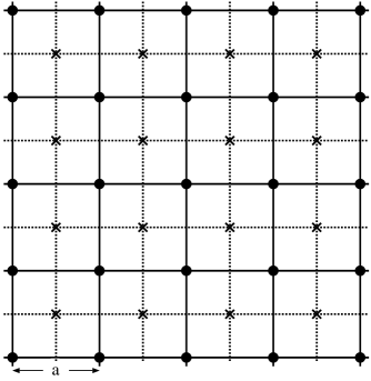
Figure 1: $\Phi_{1}(\vec{x})$ takes the same value $c_{1}$ in both $\bullet$ and $\times$ points, while $\Phi_{2}(\vec{x})$ takes the value $+c_{2}$ in the $\bullet$ points and $-c_{2}$ in the $\times$ points. Adjoining $\bullet$ and $\times$ points are joined by the fermionic links which are not shown in the figure.

The extended lattice is then made by two copies of the cubic lattice, in fact by the original lattice ( $n$ and $m$ even) and its dual ($n$ and $m$ odd) connected by the “fermionic” links $(\vec{x},\vec{x}+\vec{a}_{A})$. It is clear that there are two independent field configurations on the extended lattice that are invariant under translation, namely:

$$\Phi_{1}(\vec{x})=c_{1}~{}~{}~{}~{}~{}~{}~{}~{}~{}~{}~{},~{}~{}~{}~{}~{}~{}~{}~{}~{}~{}\Phi_{2}(\vec{x})=(-1)^{n}c_{2},$$ (2.3)

with $c_{1}$ and $c_{2}$ constant.

It is interesting to note that this phase remind us of the phase of staggered fermion [2] This is relevant because we expect the degrees of freedom of the theory in the continuum limit to be associated to small fluctuations around translationally invariant vacua, so that fluctuations around the two configurations of eq. (2.3) will correspond to two distinct degrees of freedom in the continuum limit. Hence one degree of freedom on the extended lattice will absorb two degrees of freedom of the continuum theory. This fact, namely that the extended lattice implies a correspondingly reduced number of independent fields, was not fully appreciated in the original formulation of the link approach and is one of the key points of the present paper. It is clear that since the different copies of the hyper cubic lattice in an extended lattice are generated by the extra links associated to supersymmetry charges it is natural to expect the different continuum degrees of freedom associated to a single lattice degree of freedom to be part of a supersymmetric multiplet. It is instructive to look at the previous example from the point of view of the momentum space representation, which will play a crucial role in what follows. The first Brillouin zone associated to the lattice (2.2) is the square defined by $-\frac{2\pi}{a}\leq p_{1}+p_{2}\leq\frac{2\pi}{a}$ and $-\frac{2\pi}{a}\leq p_{1}-p_{2}\leq\frac{2\pi}{a}$. That means that in the momentum space fields will be periodic with period $\frac{4\pi}{a}$ in the variables $p_{1}+p_{2}$ and $p_{1}-p_{2}$. The translationally invariant field configurations (2.7) correspond respectively to the center of the square, namely $\vec{p}=0$, and to the four vertices (which are all equivalent due to the periodicity), namely $\vec{p}=(\pm\frac{2\pi}{a},0)$ or $\vec{p}=(0,\pm\frac{2\pi}{a})$. The latter is exaclty the species doubler. A solution of the fermion doubling problem becomes now possible. Fermion doubling originates from the fact that the fermionic kinetic term has a simple zero at $\vec{p}=0$ and hence has to vanish somewhere else in the Brillouin zone due to the lattice periodicity. Within the extended lattice scheme if the second zero occurs in correspondence of the other translationally invariant vacuum the would be doubler can be interpreted as a physical field, in fact as a supersymmetric partner of the original one at $\vec{p}=0$.

We have used the example of the extended lattice of the $N=2$, $D=2$ supersymmetry to illustrate the ideas that we are going to develop in this paper. However the explicit example that we are going to study is a simpler one, $N=2$ supersymmetric model in one dimension ($D=1$). Before going into that we are going to consider an even simpler example, that has been considered in the present context in ref.  [29]. This is a one dimensional model with an $N=1$ supersymmetry. It is described in terms of a superfield:

$$\Phi(x,\theta)=\varphi(x)+i\theta\psi(x),$$ (2.4)

with a supersymmetry charge given by:

$$Q=\frac{\partial}{\partial\theta}+i\theta\frac{\partial}{\partial x},$$ (2.5)

and

$$Q^{2}=i\frac{\partial}{\partial x}.$$ (2.6)

On the lattice derivatives are replaced by finite shifts of length $a$, hence consistency with the algebra (2.6) requires that the supercharge $Q$ is associated to a shift $\frac{a}{2}$ . The extended lattice is then a one dimensional lattice with spacing $\frac{a}{2}$, which can be thought of as the superposition of two lattices with spacing $a$ each invariant under translations and separated by a an $\frac{a}{2}$ shift associated to the SUSY charge. Again there are two field configurations invariant under translations, namely:

$$\Phi_{1}(x)=c_{1}~{}~{}~{}~{}~{}~{}~{}~{}~{}~{}~{},~{}~{}~{}~{}~{}~{}~{}~{}~{}~{}\Phi_{2}(x)=(-1)^{\frac{2x}{a}}c_{2}$$ (2.7)

with $x=\frac{na}{2}$. According to the previous discussion fluctuations around $\Phi_{1}(x)$ and $\Phi_{2}(x)$ will describe in the continuum limit two distinct degrees of freedom. However we have just two degrees of freedom in this model, one bosonic and one fermionic, so the natural thing is to associate the bosonic degree of freedom to fluctuations around $\Phi_{1}(x)$ and the fermionic one to fluctuations around $\Phi_{2}(x)$.

To understand the origin of the hyper lattice structure of half lattice step and the alternating sign states, let us look at the algebraic relation of the superfield and the supercharge from a matrix point of view [15]. We now introduce the following matrix form of the super coordinate and its derivative as:

$$\theta=\begin{pmatrix}0&1\\ 0&0\end{pmatrix},~{}~{}~{}~{}~{}~{}~{}~{}~{}~{}~{}~{}~{}~{}~{}~{}~{}\frac{\partial}{\partial\theta}=\begin{pmatrix}0&0\\ 1&0\end{pmatrix},$$ (2.8)

which satisfy the following anticommutation relation:

$$\{\frac{\partial}{\partial\theta}~{},~{}\theta\}~{}=~{}1.$$ (2.9)

We may consider this matrix structure as an internal structure of the space time coordinate. With respect to this internal structure the boson $\varphi$ is considered as a field which commutes with $\theta$ and $\frac{\partial}{\partial\theta}$ and the fermion $\psi$ as a field which anticommutes with them. The component fields of boson and fermion with respect to this internal structure has then the following form:

$$\varphi(x)=\begin{pmatrix}\varphi(x)&0\\ 0&\varphi(x)\end{pmatrix},$$ (2.10)

$$\psi(x)=\begin{pmatrix}\psi(x)&0\\ 0&-\psi(x)\end{pmatrix}.$$ (2.11)

In the matrix formulation of fields the coordinate dependence can be introduced by diagonal entries of a big matrix as direct product to the internal matrix structure [15]. From the degrees of freedom point of view for N=1 model in one dimension two fields of boson and fermion on the same lattice site have this internal matrix structure (2.10) and (2.11). If we consider the $N=2$ model in one dimension, which we will consider later in this paper, there are four independent fields on one site we may then consider that the four fields of internal matrix structure may be identified with the four independent d.o.f. of fields.

We now ask a question: “How do we interpret this internal space time structure on the lattice ?” A natural identification is an introduction of a half lattice step structure to make a correspondence with two translational invariant states in (2.7). We can then identify a constant field of $\varphi(x)$ in (2.10) as $\Phi_{1}(x)$ in (2.7) and a constant field of $\psi(x)$ in (2.11) as $\Phi_{2}(x)$ in (2.7).

One can then write a lattice “superfield” corresponding to (2.4) as

$$\Phi(x)=\varphi(x)+\frac{1}{2}(-1)^{\frac{2x}{a}}\psi(x),$$ (2.12)

where we have introduced a factor $\frac{1}{2}$ for later convenience and taken away the factor $i$ since the second term is not a product of two Grassmann numbers to keep hermiticity. Since $\theta$ and $\frac{\partial}{\partial\theta}$ are not Hermitian by them self in this matrix representation we have to take care the hermiticity separately. It is crucial to recognize at this stage that the super coordinate structure and fermionic nature of $\psi$ can be accommodated by the alternating sign factor of half lattice spacing if this simple lattice representation works as a superfield. We now introduce a matrix form of a fermionic super parameter by

$$\alpha=\begin{pmatrix}\alpha&0\\ 0&-\alpha\end{pmatrix},$$ (2.13)

where $\alpha$ is a Grassmann odd parameter. This parameter can then be expressed as $\alpha(-1)^{\frac{2x}{a}}$ in accordance with the representation of the lattice superfield in (2.12).

We now propose lattice supersymmetry transformations as a finite difference over a half lattice spacing $\frac{a}{2}$:

$$\delta\Phi(x)=a^{-\frac{1}{2}}\alpha(-1)^{\frac{2x}{a}}\left(\Phi(x+\frac{a}{2})-\Phi(x)\right).$$ (2.14)

In terms of the component fields the supersymmetry transformations (2.14) are:

$$\delta\varphi(x)=-\frac{\alpha}{2}\bigg{[}\psi(x+\frac{a}{2})+\psi(x)\bigg{]}\xrightarrow[a\to 0]{}-\alpha\psi(x)\,,$$ (2.15)

$$\delta\psi(x)=2a^{-1}\alpha\bigg{[}\varphi(x+\frac{a}{2})-\varphi(x)\bigg{]}\xrightarrow[a\to 0]{}\alpha\frac{\partial\varphi(x)}{\partial x}\,.$$ (2.16)

It is surprising that the half lattice translation together with alternating sign structure (staggered phase) for the lattice superfields generates a correct lattice supersymmetry transformation. We consider that this observation is a key of our formulation.

Although supersymmetry transformations (2.15) and (2.16) have the correct structure, they violate hermiticity: a factor $i$ is missing at the l.h.s. of (2.15). In order to restore the hermiticity of the supersymmetry transformations symmetric finite differences must be used, introducing a shift of $\frac{a}{4}$ of the fermionic fields sites with respect to the bosonic ones. Hence, instead of writing the superfield on the lattice as in (2.12) we shall introduce $\Phi(x)$, with $x=n\frac{a}{4}$, defined by:

$$\Phi(x)=\left\{\begin{array}[]{lc}&\varphi(x)~{}~{}~{}~{}~{}~{}~{}~{}\textrm{for}~{}~{}~{}x=na/2,\\ &\frac{1}{2}a^{1/2}e^{\frac{2i\pi x}{a}}\psi(x)~{}~{}~{}\textrm{for}~{}~{}~{}x=(2n+1)a/4.\end{array}\right.$$ (2.17)

Again the supersymmetry transformations can be written in terms of $\Phi(x)$:

$$\delta\Phi(x)=\alpha a^{-1/2}e^{\frac{2i\pi x}{a}}\left[\Phi(x+a/4)-\Phi(x-a/4)\right].$$ (2.18)

By separating $\Phi(x)$ into its component fields according to (2.17) we find:

$$\delta\varphi(x)=\frac{i\alpha}{2}\bigg{[}\psi(x+\frac{a}{4})+\psi(x-\frac{a}{4})\bigg{]}\xrightarrow[a\to 0]{}i\alpha\psi(x)\,,$$ (2.19)

$$\delta\psi(x)=2a^{-1}\alpha\bigg{[}\varphi(x+\frac{a}{4})-\varphi(x-\frac{a}{4})\bigg{]}\xrightarrow[a\to 0]{}\alpha\frac{\partial\varphi(x)}{\partial x}\,,$$ (2.20)

where $x$ is an even multiple of $a/4$ in (2.19) and an odd one in (2.20). As in the continuum case the commutator of two SUSY transformation is a translation, namely, on the lattice, a finite difference of spacing $a$. For instance we have for $\varphi(x)$ (the same applies to $\psi(x)$):

$$\delta_{\beta}\delta_{\alpha}\varphi(x)-\delta_{\alpha}\delta_{\beta}\varphi(x)=\frac{2i\alpha\beta}{a}\left[\varphi(x+a/2)-\varphi(x-a/2)\right].$$ (2.21)

It is instructive to look at the supersymmetry transformations given above from the point of view of of the momentum space representation. Let us consider first the Fourier transform of the component fields $\psi(x)$ and $\varphi(x)$, and denote them by $\tilde{\psi}(p)$ and $\tilde{\varphi}(p)$ respectively. The lattice spacing being $a/2$, the Brillouin zone extends over a $\frac{4\pi}{a}$ interval with the two vacua $\Phi_{1}(x)$ and $\Phi_{2}(x)$ corresponding respectively to $p=0$ and $p=\frac{2\pi}{a}$. The periodicity conditions are:

$$\tilde{\varphi}(p+\frac{4\pi}{a})=\tilde{\varphi}(p),\,\,\,\,\,\,\,\tilde{\psi}(p+\frac{4\pi}{a})=-\tilde{\psi}(p),$$ (2.22)

where the minus sign in the case of $\tilde{\psi}$ is due to the $a/4$ shift in coordinate space of the fermionic field. The supersymmetry transformations (2.19) and (2.20) are then given by:

$$\delta\tilde{\varphi}(p)=i\cos\frac{ap}{4}\,\alpha\tilde{\psi}(p),$$ (2.23)

$$\delta\tilde{\psi}(p)=-i\frac{4}{a}\sin\frac{ap}{4}\,\alpha\tilde{\varphi}(p).$$ (2.24)

Eqs. (2.23) and (2.24) are consistent with both the periodicity conditions (2.22) and with the reality conditions expressed in momentum space by: $\tilde{\varphi}(p)^{\dagger}=\tilde{\varphi}(-p)$ and $\tilde{\psi}(p)^{\dagger}=\tilde{\psi}(-p)$. A more extensive analysis of the $D=1$, $N=1$ model, including the lattice action, can be found in  [29]. The point we want to emphasize here is the following: in order to derive the supersymmetry transformations (2.19) and (2.20), or equivalently their momentum space representation (2.23) and (2.24), we started from a bosonic field $\varphi(x)$ and a fermionic one $\psi(x)$ interpreted respectively as fluctuations around $\Phi_{1}(x)$ (i.e. $p=0$) and $\Phi_{2}(x)$ (i.e $p=\frac{2\pi}{a}$). Either these two fields represent on the lattice a single degree of freedom whose statistic changes from bosonic to fermionic as the momentum moves from zero to $\frac{2\pi}{a}$ ( and we don’t know how to implement that consistently) or each field has a doubler with the same statistic in correspondence of the other vacuum. In this case the system will contain two bosonic and two fermionic degrees of freedom in the continuum, for which there is no room in the $D=1$, $N=1$ supersymmetry. Furthermore the action of this model is fermionic and thus the vacuum is not well defined. We will show in the following section that it actually provides a consistent formulation of the $D=1$, $N=2$ supersymmetry , whose algebra contains a bosonic field $\varphi$ and a bosonic auxiliary field $D$, described by the lattice bosonic field at $p=0$ and $p=\frac{2\pi}{a}$ respectively and, in the fermionic sector, two fields $\psi_{1}$ and $\psi_{2}$ described on the lattice by the fluctuations of a single field around the two vacua. We will show in the following sections that the $N=2$ supersymmetry can be explicitly formulated on the lattice (one of the transformations is essentially already given in (2.23) and (2.24) ), an invariant action can be constructed (including the mass and interaction term) and the continuum limit taken keeping exact supersymmetry at all stages. The doubling problem does not arise since the would be doublers are physical degrees of freedom in the same supermultiplet as the original field.

3 The model

We briefly summarize the continuum version of one dimensional $N=2$ supersymmetric model with two supersymmetry charges $Q_{1}$ and $Q_{2}$ [13], whose matrix version on the lattice was discussed in  [15]. Its supersymmetry algebra is given by:

$$Q_{1}^{2}=Q_{2}^{2}=P_{t},~{}~{}~{} ~{}~{}~{}\{Q_{1},Q_{2}\}=0,$$ (3.1)

$$[P_{t},Q_{1}]= [P_{t},Q_{2}]=0,$$ (3.2)

where $P_{t}$ is the generator of translations in the one-dimensional space-time coordinate $t$:

$$P_{t}=-i\frac{\partial}{\partial t}.$$ (3.3)

A superspace representation of the algebra may be given in terms of two Grassmann odd, real coordinates $\theta_{1}$ and $\theta_{2}$, namely:

$$Q_{1}=\frac{\partial}{\partial\theta_{1}}-i\theta_{1}\frac{\partial}{\partial t},~{}~{}~{}~{}~{}~{}~{}~{}~{}~{}Q_{2}=\frac{\partial}{\partial\theta_{2}}-i\theta_{2}\frac{\partial}{\partial t}.$$ (3.4)

The field content of the theory is described by a hermitian superfield $\Phi(t,\theta_{1},\theta_{2})$:

$$\Phi(t,\theta_{1},\theta_{2})=\varphi(t)+i\theta_{1}\psi_{1}(t)+i\theta_{2}\psi_{2}(t)+i\theta_{2}\theta_{1}D(t),$$ (3.5)

where $\psi_{1}$ and $\psi_{2}$ are Majorana fermions. The supersymmetry transformations of the superfield $\Phi$ are given by:

$$\delta_{j}\Phi=[\eta_{j}Q_{j},\Phi]~{}~{}~{}~{}~{}~{}~{}~{}~{}~{}j=1,2,$$ (3.6)

where $\eta_{i}$ are the Grassmann odd parameters of the transformation. In terms of the component fields eq. (3.6) reads:

$$\delta_{j}\varphi =i\eta_{j}\psi_{j},$$ (3.7)

$$\delta_{j}\psi_{k} =\delta_{j,k}\eta_{j}\partial_{t}\varphi+\epsilon_{jk}\eta_{j}D,$$ (3.8)

$$\delta_{j}D =i\epsilon_{jk}\eta_{j}\partial_{t}\psi_{k}.$$ (3.9)

It is important to note that since the supersymmetry transformations are defined in (3.6) as commutators, supersymmetry transformations of superfields products obey Leibniz rule:

$$\delta_{i}(\Phi_{1}\Phi_{2})=(\delta_{i}\Phi_{1})\Phi_{2}+\Phi_{1}(\delta_{i}\Phi_{2}).$$ (3.10)

In order to write a supersymmetric action we need to introduce the super derivatives, defined as

$$D_{j}=\frac{\partial}{\partial\theta_{j}}+i\theta_{j}\frac{\partial}{\partial t},$$ (3.11)

which anticommute with the supersymmetry charges $Q_{j}$ and satisfy the algebra:

$$D_{j}^{2}=i\frac{\partial}{\partial t},~{}~{}~{}~{}~{}~{}~{}~{}~{}~{}\{D_{1},D_{2}\}=0.$$ (3.12)

The supersymmetric action can then be defined in terms of the superfield $\Phi$ as:

$$\int dtd\theta_{1}d\theta_{2}\left[\frac{1}{2}D_{2}\Phi D_{1}\Phi+iV(\Phi)\right],$$ (3.13)

where $V(\Phi)$ is a superpotential which may includes any powers of superfields together with coupling constants. By integrating over $\theta_{1}$ and $\theta_{2}$ in (3.13) one can obtain the action written in terms of the component fields. If we take the super potential in the following form:

$$V(\Phi)=\frac{1}{2}m\Phi^{2}+\frac{1}{4}g\Phi^{4},$$ (3.14)

we obtain the following action:

$$S= \int dt\{\frac{1}{2}\left[-(\partial_{t}\varphi)^{2}-D^{2}+i\psi_{1}\partial_{t}\psi_{1}+i\psi_{2}\partial_{t}\psi_{2}\right]$$

$$- m(i\psi_{1}\psi_{2}+D\varphi)-g(3i\varphi^{2}\psi_{1}\psi_{2}+D\varphi^{3})\}.$$ (3.15)

As we can see, the general interaction terms in $\Phi^{n}$ are of the forms of $\varphi^{n-2}\psi_{1}\psi_{2}$ and $D\varphi^{n-1}$.

It is convenient for later use to write the SUSY transformations in the Lorentzian metric and in the momentum representation. They are given by:

$$\delta_{1}\varphi(p) =i\eta_{1}\psi_{1}(p), \delta_{2}\varphi(p) =i\eta_{2}\psi_{2}(p),$$

$$\delta_{1}\psi_{1}(p) =-i\eta_{1}p\varphi(p), \delta_{2}\psi_{1}(p) =-\eta_{2}D(p),$$

$$\delta_{1}\psi_{2}(p) =\eta_{1}D(p), \delta_{2}\psi_{2}(p) =-i\eta_{2}p\varphi(p),$$

$$\delta_{1}D(p) =\eta_{1}p\psi_{2}(p), \delta_{2}D(p) =-\eta_{2}p\psi_{1}(p).$$ (3.16)

Notice that $\delta_{2}$ is obtained from $\delta_{1}$ with the discrete symmetry: $\psi_{1}\rightarrow\psi_{2}$ an $\psi_{2}\rightarrow-\psi_{1}$. Finally we write the action in the momentum representation:

$$S= \int dp\Bigl{\{}\frac{1}{2}\left[-p^{2}\varphi(-p)\varphi(p)-D(-p)D(p)+i\psi_{1}(-p)p\psi_{1}(p)+i\psi_{2}(-p)p\psi_{2}(p)\right]$$

$$- m(i\psi_{1}(-)\psi_{2}(p)+D(-p)\varphi(p))\Bigr{\}}$$

$$- g\int dp_{1}dp_{2}dp_{3}dp_{4}(3i\varphi(p_{1})\varphi(p_{2})\psi_{1}(p_{3})\psi_{2}(p_{4})+D(p_{1})\varphi(p_{2})\varphi(p_{3})\varphi(p_{4}))\delta(p_{1}+p_{2}+p_{3}+p_{4}).$$ (3.17)

4 Supersymmetry transformations on the lattice

According to the discussion of section 2 the formulation of the $D=1$, $N=2$ supersymmetric model on a lattice with spacing $\frac{a}{2}$ should involve on the lattice two fields, one bosonic and one fermionic. In fact the lattice consists of two sub lattices with lattice spacing $a$ invariant under translations and hence each degree of freedom on the lattice corresponds to two degrees of freedom in the continuum limit. Let us denote the bosonic “superfield” by $\Phi(x)$ with $x=\frac{na}{2}$, and the fermionic “superfield” by $\Psi(x)$ with $x=\frac{na}{2}+\frac{a}{4}$. The shift of $\frac{a}{4}$ in the fermionic superfield with respect to the bosonic one has been introduced to have symmetric finite differences in the supersymmetry transformations and implement hermiticity in a natural way as discussed in section 2. A picture of the lattice is given in fig. 2.

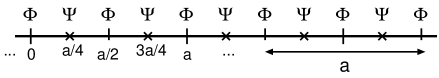
Figure 2: One dimensional lattice with the bosonic field $\Phi$ located on the points multiple of $\frac{a}{2}$, and the fermionic field $\Psi$ on points shifted by $\frac{a}{4}$.

Let us proceed now to define the supersymmetry transformations on the lattice. There are two supercharges in the $N=2$ model, whose algebra was given in (3.1). One of the supersymmetry transformation, which we shall denote by $\delta_{1}$, was already formulated on the lattice in the context of the $N=1$ model and can be written as:

$$\delta_{1}\Phi(x)=\frac{i\alpha}{2}\bigg{[}\Psi(x+\frac{a}{4})+\Psi(x-\frac{a}{4})\bigg{]}~{}~{}~{}~{}~{}~{}~{}~{}x=\frac{na}{2}\,,$$ (4.1)

$$\delta_{1}\Psi(x)=2\alpha\bigg{[}\Phi(x+\frac{a}{4})-\Phi(x-\frac{a}{4})\bigg{]}~{}~{}~{}~{}~{}~{}~{}~{}~{}x=\frac{na}{2}+\frac{a}{4}\,.$$ (4.2)

We assume here that $\Phi(x)$ and $\Psi(x)$ are dimensionless, so that no dependence on the lattice spacing $a$ appears at the r.h.s. of (4.1) and (4.2). Of course a rescaling of the fields with powers of $a$ will be needed to make contact with the fields of the continuum theory. Let us introduce now the superfields in the momentum space defined as the Fourier transform of $\Phi(x)$ and $\Psi(x)$:

$$\Phi(p)=\frac{1}{2}\sum_{x=\frac{na}{2}}e^{ipx}\Phi(x),\,~{}~{}~{}~{}~{}~{}~{}~{}~{}~{}~{}~{}~{}~{}~{}~{}~{}~{}\,\Psi(p)=\frac{1}{2}\sum_{x=\frac{na}{2}+\frac{a}{4}}e^{ipx}\Psi(x).\,$$ (4.3)

The corresponding inverse transformations are:

$$\Phi(x)=a\int_{0}^{\frac{4\pi}{a}}\frac{dp}{2\pi}\Phi(p)e^{-ipx},\,~{}~{}~{}~{}~{}~{}~{}~{}~{}~{}~{}~{}~{}~{}~{}~{}~{}~{}\,\Psi(x)=a\int_{0}^{\frac{4\pi}{a}}\frac{dp}{2\pi}\Psi(p)e^{-ipx}.\,$$ (4.4)

From(4.3) it is clear that $\Phi(p)$ and $\Psi(p)$ satisfy the following periodicity conditions:

$$\Phi(p+\frac{4\pi}{a})=\Phi(p),\,~{}~{}~{}~{}~{}~{}~{}~{}~{}~{}~{}~{}~{}~{}~{}~{}~{}~{}\Psi(p+\frac{4\pi}{a})=-\Psi(p).$$ (4.5)

In momentum representation the supersymmetry transformations (4.1) and (4.2) read:

$$\delta_{1}\Phi(p)=i\cos\frac{ap}{4}\alpha\Psi(p)\,,$$ (4.6)

$$\delta_{1}\Psi(p)=-4i\sin\frac{ap}{4}\alpha\Phi(p)\,.$$ (4.7)

The commutator of two supersymmetry transformations $\delta_{1}$ with parameters $\alpha$ and $\beta$ defines an infinitesimal translation on the lattice. From (4.6) and (4.7) one finds:

$$\delta_{1\beta}\delta_{1\alpha}F(p)-\delta_{1\alpha}\delta_{1\beta}F(p)=4\sin\frac{ap}{2}\alpha\beta F(p),$$ (4.8)

where $F(p)$ stands for either $\Phi(p)$ or $\Psi(p)$. In coordinate space this is completely equivalent to (2.21), so that an infinitesimal translation of parameter $\lambda$ on the lattice is defined by;

$$F(x)\rightarrow F(x)+\lambda\frac{F(x+\frac{a}{2})-F(x-\frac{a}{2})}{a},$$ (4.9)

which clearly reduces to $F(x)\rightarrow F(x+\lambda)$ in the continuum limit. Translations defined in (4.9) are however conceptually different from the discrete translations on the lattice that would be defined as:

$$F(x)\rightarrow F(x+a)=F(x)+a\frac{F(x+a)-F(x)}{a}.$$ (4.10)

The difference between the two definitions is even more apparent in the momentum representation, where (4.10) is simply $F(p)\rightarrow e^{iap}F(p)$ and applied to a product of fields leads to the standard form of momentum conservation. Invariance under (4.9) instead leads to a non local conservation law where $p$ is replaced by $\sin\frac{ap}{2}$, namely , for a product of fields of momenta $p_{1}$,$p_{2}$,…,$p_{n}$:

$$\sin\frac{ap_{1}}{2}+\sin\frac{ap_{2}}{2}+\cdots+\sin\frac{ap_{n}}{2}=0.$$ (4.11)

This conservation law on the lattice was first pointed out by Dondi and Nicolai [16]. The implications of this conservation law, in particular with respect to the validity of the Leibniz rule and the relation of the present approach to the link approach will be discussed in section 7. In the continuum limit ($ap_{i}\ll 1$) (4.11) reduces to the standard momentum conservation law and locality is restored. The conservation law (4.11) is not affected if any momentum $p_{i}$ in it is replaced by $\frac{2\pi}{a}-p_{i}$ due to the invariance of the sine. In view of last section’s discussion the interpretation is clear: in the continuum limit ( $ap\ll 1$) $F(p)$ and $F(\frac{2\pi}{a}-p)$ represent fluctuations of momentum $p$ respectively around the vacuum of momentum zero and $\frac{2\pi}{a}$ on the lattice. So the symmetry $p\rightarrow\frac{2\pi}{a}-p$ amounts to exchanging the two vacua keeping the physical momentum unchanged and will play an important role in supersymmetry transformations.

We now want to match the superfields $\Phi(p)$ and $\Psi(p)$ appearing in the supersymmetry transformations (4.6) and (4.7) with the component fields of the $N=2$ $D=1$ supersymmetry described in the previous section. Working in the momentum representation we shall associate $\varphi$ and $D$ with the fluctuations of $\Phi$ respectively around $0$ and $\frac{2\pi}{a}$ and similarly $\psi_{1}$ and $\psi_{2}$ with the fluctuations of $\Psi$. More specifically we assume the following correspondence:

$$\Phi(p)=a^{-\frac{3}{2}}\varphi(p),$$ (4.12)

$$\Psi(p)=a^{-1}\psi_{1}(p),$$ (4.13)

$$\Psi(\frac{2\pi}{a}-p)=ia^{-1}\psi_{2}(p),$$ (4.14)

$$\Phi(\frac{2\pi}{a}-p)=-\frac{a^{-\frac{1}{2}}}{4}D(p),$$ (4.15)

where $p$ is restricted in (4.12-4.15) to the interval $(-\frac{\pi}{a},\frac{\pi}{a})$, which is also the range of definition of the component fields (although with a possible discontinuity at $p=\pm\frac{\pi}{a}$) which corresponds to a lattice of spacing $a$. A rescaling of the fields with powers of $a$ has been also introduced in (4.12-4.15) to account for the dimensionality of the component fields in momentum representation (remember that $\Phi$ and $\Psi$ were defined to be dimensionless). A similar rescaling will be assumed for the supersymmetry parameter $\alpha$:

$$\alpha=a^{\frac{1}{2}}\eta.$$ (4.16)

By inserting (4.12-4.15) and (4.16) into the supersymmetry transformations (4.6) and (4.7) we obtain for the component fields the following transformations:

$$\delta_{1}\varphi(p)=i\cos\frac{ap}{4}\eta\psi_{1}(p) \underset{ap\ll 1}{\longrightarrow} i\eta\psi_{1}(p),$$ (4.17)

$$\delta_{1}\psi_{1}(p)=-i\frac{4}{a}\sin\frac{ap}{4}\eta\varphi(p) \underset{ap\ll 1}{\longrightarrow} -ip\eta\varphi(p),$$ (4.18)

$$\delta_{1}\psi_{2}(p)=\cos\frac{ap}{4}\eta D(p) \underset{ap\ll 1}{\longrightarrow} \eta D(p),,$$ (4.19)

$$\delta_{1}D(p)=\frac{4}{a}\sin\frac{ap}{4}\eta\psi_{2}(p) \underset{ap\ll 1}{\longrightarrow} p\eta\psi_{2}(p).$$ (4.20)

In the continuum limit $ap\ll 1$ the above supersymmetry transformations on the lattice reproduce exactly the ones in the continuum (3.16) given in Section 3. As already mentioned after eq. (4.15), the momentum $p$ appearing as the argument of the component fields in (4.12-4.15) and in (4.17-4.20) is restricted to the interval $(-\frac{\pi}{a},\frac{\pi}{a})$. So we could introduce a lattice of spacing $a$ and coordinates $\tilde{x}=na$ and define the component fields $\varphi(\tilde{x})$, etc. on such lattice by taking the Fourier transform on the $\frac{2\pi}{a}$ interval of $\varphi(p)$, etc. and finally write the supersymmetry transformations (4.17-4.20) of the component fields in the $\tilde{x}$ coordinate representation. However the trigonometric functions at the r.h.s. of (4.17-4.20) are not periodic of period $\frac{2\pi}{a}$, and as a result the supersymmetry transformation are non-local in the $\tilde{x}$ coordinate representation, implying that the natural representation for the supersymmetry is on the lattice with $\frac{a}{2}$ spacing.

We have now to identify the second supersymmetry transformation $\delta_{2}$. In the continuum $\delta_{2}$ is obtained from $\delta_{1}$ by replacing everywhere $\psi_{1}(p)$ with $\psi_{2}(p)$, and $\psi_{2}(p)$ with $-\psi_{1}(p)$. It is easy to see from (4.12-4.15) that this corresponds on the lattice to the replacement:

$$\Psi(p)\longrightarrow-i\Psi(\frac{2\pi}{a}-p).$$ (4.21)

By performing this replacement on the supersymmetry transformations (4.6) and (4.7) one obtains the expression for $\delta_{2}$:

$$\delta_{2}\Phi(p)=\cos\frac{ap}{4}\alpha\Psi(\frac{2\pi}{a}-p)\,,$$ (4.22)

$$\delta_{2}\Psi(\frac{2\pi}{a}-p)=4\sin\frac{ap}{4}\alpha\Phi(p)\,.$$ (4.23)

The supersymmetry transformation $\delta_{2}$, defined by (4.22) and (4.23), satisfies together with $\delta_{1}$ an $N=2$ supersymmetry algebra. It is easy to check in fact that the commutator of two $\delta_{2}$ transformations gives an infinitesimal translation ( namely eq. (4.8) holds also for $\delta_{2}$) and that the commutator of a $\delta_{1}$ and $\delta_{2}$ transformation vanishes, namely:

$$\delta_{1\beta}\delta_{2\alpha}F(p)-\delta_{2\alpha}\delta_{1\beta}F(p)=0.$$ (4.24)

In terms of the component fields, and in the continuum limit, the explicit expression for the $\delta_{2}$ transformation can be obtained from (4.22) and (4.23) by using eq.s (4.12-4.15):

$$\delta_{2}\varphi(p)=i\cos\frac{ap}{4}\eta\psi_{2}(p) \underset{ap\ll 1}{\longrightarrow} i\eta\psi_{2}(p),$$ (4.25)

$$\delta_{2}\psi_{2}(p)=-i\frac{4}{a}\sin\frac{ap}{4}\eta\varphi(p) \underset{ap\ll 1}{\longrightarrow} -ip\eta\varphi(p),$$ (4.26)

$$\delta_{2}\psi_{1}(p)=-\cos\frac{ap}{4}\eta D(p) \underset{ap\ll 1}{\longrightarrow} -\eta D(p),$$ (4.27)

$$\delta_{2}D(p)=-\frac{4}{a}\sin\frac{ap}{4}\eta\psi_{1}(p) \underset{ap\ll 1}{\longrightarrow} -p\eta\psi_{1}(p).$$ (4.28)

As for $\delta_{1}$ in the limit $ap\ll 1$ the above transformation coincides, in the momentum space representation, with the one generated by $Q_{2}$ in the continuum theory.

The coordinate representation of $\delta_{2}$ can be obtained directly from (4.25-4.28) by Fourier transform, or from (4.1-4.2) by performing the following substitution:

$$\Psi(x)\longrightarrow(-1)^{n}\Psi(-x)~{}~{}~{}~{}~{}~{}~{}~{}~{}~{}~{}~{}x=\frac{na}{2}-\frac{a}{4},~{}~{}~{}~{}~{}~{}~{}~{}~{}~{}~{}~{}~{}$$ (4.29)

which is the same as (4.21) in the coordinate representation. Either way the result is:

$$\delta_{2}\Phi(x)=\frac{i\alpha}{2}(-1)^{n}\bigg{[}\Psi(-x+\frac{a}{4})-\Psi(-x-\frac{a}{4})\bigg{]}~{}~{}~{}~{}~{}~{}~{}~{}x=\frac{na}{2}\,,$$ (4.30)

$$\delta_{2}\Psi(x)=2\alpha(-1)^{n}\bigg{[}\Phi(-x+\frac{a}{4})-\Phi(-x-\frac{a}{4})\bigg{]}~{}~{}~{}~{}~{}~{}~{}~{}~{}x=\frac{na}{2}+\frac{a}{4}\,.$$ (4.31)

It is clear from (4.30) and (4.31) that the supersymmetry transformation $\delta_{2}$ is local in the coordinate representation only modulo the reflection $x\rightarrow-x$. This was already implicit in the correspondence (4.12-4.15) between the lattice fields and the ones of the continuum theory. In fact it is clear from (4.12-4.15) that while for instance $\varphi(x)$ is associated to the fluctuations of $\Phi(x)$ around the constant configuration ($p=0$), the fluctuations of $\Phi(x)$ around the constant configuration with alternating sign ($p=\frac{2\pi}{a}$) correspond in the continuum to $D(-x)$. For fermions this parity change leads to a physical meaning. Since $\psi_{2}(p)\leftrightarrow\psi_{2}(x)$ is defined as a species doubler of $\psi_{1}(p)\leftrightarrow\psi_{1}(x)$, the chirality of $\psi_{2}$ is the opposite of $\psi_{1}$. However by the change of $p\rightarrow\frac{2\pi}{a}-p$ equivalently $x\rightarrow-x$, chirality of $\psi_{1}$ and $\psi_{2}$ are adjusted to be the same. Thus this bi local nature in the coordinate space may be transfered to a local interpretation.

5 Supersymmetric invariant action

In order to construct a lattice action invariant under the two supersymmetry transformations $\delta_{1}$ and $\delta_{2}$ defined in the previous section we consider first the invariance under translations, which follows from supersymmetry, and it is expressed by the sine conservation law given in (4.11).

Any vertex of a supersymmetric invariant theory will have to include a delta function enforcing the conservation law (4.11). Unlike the standard momentum conservation this conservation law does not lead to a local action in coordinate space, and in fact it makes it impossible to write the action in coordinate space without using transcendental function (more specifically Bessel functions). For this reason we shall first formulate the action in the momentum representation. We provide a full treatment of coordinate prescription later in section 7. There is however an important exception to this, namely the case $n=2$, that is the kinetic term and the mass term. In fact for $n=2$ the conservation law (4.11) has two solutions:

$$p_{1}+p_{2}=0~{}~{}~{}~{}~{}~{}~{}~{}~{}~{}~{}~{}~{}~{}~{}~{}~{}~{}({\rm mod}~{}~{}~{}~{}\frac{4\pi}{a})$$ (5.1)

and

$$p_{1}-p_{2}=\frac{2\pi}{a}~{}~{}~{}~{}~{}~{}~{}~{}~{}~{}~{}~{}~{}~{}~{}~{}~{}~{}({\rm mod}~{}~{}~{}~{}\frac{4\pi}{a})$$ (5.2)

and the delta function of momentum conservation does not need in this case to include any sine function. The two point term in the action with the momentum conservation (5.1) describes, as we shall see, the kinetic term and is local when expressed in the coordinate representation. The mass term will be expressed instead by a term with the conservation law (5.2), involving in coordinate space a coupling between fields in $x$ and $-x$, in agreement with the discussion at the end of the previous section. Let us introduce now a supersymmetric action on the lattice. All terms of this action have the same structure, which for an $n$-point term is the following:

$$S^{(n)} =g_{0}^{(n)}a^{n}\frac{4}{n!}\int_{-\frac{\pi}{a}}^{\frac{3\pi}{a}}\frac{dp_{1}}{2\pi}\cdots\frac{dp_{n}}{2\pi}2\pi\delta\left(\sum_{i=1}^{n}\sin\frac{ap_{i}}{2}\right)$$

$$\qquad\times G(p_{1},p_{2},\cdots,p_{n})\Bigl{[}2\sin^{2}\frac{ap_{1}}{4}~{}\Phi(p_{1})\Phi(p_{2})\cdots\Phi(p_{n})+$$ (5.3)

$$+\frac{n-1}{4}~{}\sin\frac{a(p_{1}-p_{2})}{4}~{}\Psi(p_{1})\Psi(p_{2})\Phi(p_{3})\cdots\Phi(p_{n})\Bigr{]}.$$

A direct check shows that $S^{(n)}$ is invariant under the supersymmetry transformation $\delta_{1}$ defined in (4.1,4.2) as well as under the replacement (4.21), which in turn implies the invariance under $\delta_{2}$ provided the otherwise arbitrary function $G$ satisfies the following properties: i) it is symmetric under permutations of the momenta $p_{i}$, ii) it is periodic with period $\frac{4\pi}{a}$ in all the momenta and iii) it is invariant when an even number of $p_{i}$ is replaced by $\frac{2\pi}{a}-p_{i}$. An example of function satisfying the above requirements is:

$$C(p)=\prod_{i=1}^{n}~{}\cos\frac{ap_{i}}{2}.$$ (5.4)

For all interaction terms ($n>2$) we will take $G(p)=C(p)$. In fact, thanks to the cosine factors the function $C(p)$ vanishes if any of the momenta $p_{i}$ is equal to $\pm\frac{\pi}{a}$, so a factor $C(p)$ is needed to cancel the singularities arising at $p_{i}=\pm\frac{\pi}{a}$ from the integration volume as a consequence of the delta function. Later in section seven we find out another natural reason why this factor (5.4) comes out. All terms in (5.3) are periodic with period $\frac{4\pi}{a}$ in the momenta, and the momentum integration is over a whole period: the specific choice here (from $\frac{-\pi}{a}$ to $\frac{3\pi}{a}$) is for future convenience. The integrand can be made explicitly symmetric with respect to permutations of the momenta, so the factor $2\sin^{2}\frac{ap_{1}}{4}$ in front of the bosonic part can be replaced by

$$2\sin^{2}\frac{ap_{1}}{4}\rightarrow 1-\frac{1}{n}\sum_{1}^{n}\cos\frac{ap_{i}}{2}.$$ (5.5)

It should be noticed also that, although we kept the dependence on the lattice spacing $a$ explicit, this could be completely absorbed in the definition of the momenta, by introducing a-dimensional momenta $\tilde{p}_{i}=ap_{i}$.

5.1 Kinetic term and Mass term

The case $n=2$ is special because only in that case the sine conservation law splits into the two separate conservation laws (5.1) and (5.2) which are linear in the momenta. The delta function in (5.3) can then be replaced by the sum, with arbitrary coefficients, of the delta functions enforcing (5.1) and (5.2). This amounts ( for $n=2$ only) to perform in (5.3) the following replacement:

$$\frac{a}{2}g_{0}^{(2)}G(p_{1},p_{2})\delta(\sin\frac{ap_{1}}{2}+\sin\frac{ap_{2}}{2})\longrightarrow\delta(p_{1}+p_{2})+m_{0}\delta(p_{1}-p_{2}-\frac{2\pi}{a}),$$ (5.6)

where $m_{0}$ is a free parameter. The delta functions at the r.h.s. of (5.6) do not give rise to any singularity at $p_{i}=\pm\frac{\pi}{a}$ so no factor $C(p)$ is required in this case We are going to show here that the first delta in (5.6) generates the supersymmetric kinetic term, the second delta the supersymmetric mass term. By inserting the r.h.s. of (5.6) into (5.3) and performing one momentum integration we obtain:

$$S^{(2)}=S_{kin}+S_{mass},$$ (5.7)

with

$$S_{kin}=4a\int_{-\frac{\pi}{a}}^{\frac{3\pi}{a}}\frac{dp}{2\pi}\left[2\sin^{2}\frac{ap}{4}\Phi(-p)\Phi(p)-\frac{1}{4}\sin\frac{ap}{2}\Psi(-p)\Psi(p)\right],$$ (5.8)

and

$$S_{mass}=4am_{0}\int_{-\frac{\pi}{a}}^{\frac{3\pi}{a}}\frac{dp}{2\pi}\left[\Phi(p+\frac{2\pi}{a})\Phi(p)+\frac{1}{4}\Psi(p+\frac{2\pi}{a})\Psi(p)\right].$$ (5.9)

One could regard the kinetic term (5.8) as the kinetic term of a lattice theory with lattice spacing $a^{\prime}=\frac{a}{2}$ and just one bosonic and one fermionic degree of freedom. The invariance under the $\delta_{1}$ supersymmetry transformations (4.6,4.7) would be described as an $N=1$ supersymmetry. However, as shown by (5.8), the fermion would have a doubler at $p=\frac{\pi}{a^{\prime}}$, as expected. Our interpretation is different. Since supersymmetry transformations (4.2) are related to shifts of $\frac{a}{2}$, we consider $a$ as the fundamental lattice spacing and the $\frac{a}{2}$ spacing as the signal that we are describing with the same lattice field two distinct degrees of freedom in the continuum: hence the fermion and its doubler are interpreted as partners in an $N=2$ supersymmetry generated by $\delta_{1}$ and $\delta_{2}$, the latter given by (4.22,4.23). In order to separate the degrees of freedom let us split the integration region in (5.8) and (5.9) into $(-\frac{\pi}{a},\frac{\pi}{a})$ and $(\frac{\pi}{a},\frac{3\pi}{a})$. In the first interval we use the correspondence (4.12,4.13), in the second the correspondence (4.14,4.15) and find:

$$S_{kin}= \int_{-\frac{\pi}{a}}^{\frac{\pi}{a}}\frac{dp}{2\pi}\Bigl{[}\frac{4}{a^{2}}(1-\cos\frac{ap}{2})\varphi(-p)\varphi(p)+\frac{1}{4}(1+\cos\frac{ap}{2})D(-p)D(p)-$$ (5.10)

$$-\frac{1}{a}\sin\frac{ap}{2}\psi_{1}(-p)\psi_{1}(p)-\frac{1}{a}\sin\frac{ap}{2}\psi_{2}(-p)\psi_{2}(p)\Bigr{]}.$$

Similarly for the mass term we get:

$$S_{mass}=2m\int_{-\frac{\pi}{a}}^{\frac{\pi}{a}}\frac{dp}{2\pi}\left[-\varphi(-p)D(p)-i\psi_{1}(-p)\psi_{2}(p)\right],$$ (5.11)

where $m$ is now the physical mass: $m=\frac{m_{0}}{a}$. Thanks to the rescaling all fields in (5.10) and (5.11) have the correct canonical dimension, and the continuum limit is smooth. The component fields $\varphi(p)$,$D(p)$,$\psi_{1}(p)$ and $\psi_{2}(p)$ are defined for $p$ in the interval $(-\frac{\pi}{a},\frac{\pi}{a})$. This is the Brillouin zone corresponding to a lattice of spacing $a$, so we could define a lattice with coordinates $\tilde{x}=na$ and the component fields on it as the Fourier transforms of the momentum space components. For instance we could define:

$$\varphi(\tilde{x})=\int_{-\frac{\pi}{a}}^{\frac{\pi}{a}}\frac{dp}{2\pi}\varphi(p)e^{-ip\tilde{x}}.$$ (5.12)

However the action written in the coordinate $\tilde{x}$ space is non-local, since the finite difference operators appearing in (5.10) are periodic with period $\frac{4\pi}{a}$ and not $\frac{2\pi}{a}$ that would be needed for a local expression on a lattice with spacing $a$.

Instead it is possible, using (4.3), to write (5.8) in the coordinate space $x$ with lattice spacing $\frac{a}{2}$:

$$S_{kin}=\sum_{x=n\frac{a}{2}}\left[\Phi(x)\left(2\Phi(x)-\Phi(x+\frac{a}{2})-\Phi(x-\frac{a}{2})\right)+\frac{i}{2}\Psi(x+\frac{a}{4})\Psi(x-\frac{a}{4})\right].$$ (5.13)

In the bosonic part of the action the equivalent of a second finite difference appears. In fact if we define the finite difference on the lattice of spacing $\frac{a}{2}$ as

$$\partial_{\pm}F(x)=F(x\pm\frac{a}{2})-F(x),$$ (5.14)

the kinetic term can be rewritten as:

$$S_{kin}=\sum_{x=n\frac{a}{2}}\left[\Phi(x)~{}\partial_{-}\partial_{+}\Phi(x)+\frac{i}{2}\Psi(x+\frac{a}{4})~{}\partial_{-}\Psi(x+\frac{a}{4})\right].$$ (5.15)

The coordinate representation for the mass term (5.9) reveals some new features, namely a coupling between fields in $x$ and $-x$. In fact, by using again (4.3), one finds:

$$S_{mass}=\frac{m_{0}}{2}\sum_{x=n\frac{a}{2}}(-1)^{\frac{2x}{a}}\left[\Phi(-x)\Phi(x)+\frac{i}{4}\Psi(-x-\frac{a}{4})\Psi(x+\frac{a}{4})\right].$$ (5.16)

The bi local structure of (5.16) shows that the extended lattice with spacing $\frac{a}{2}$ has not a straightforward relation to the coordinate space in the continuum limit. This is related to the fact that while the fluctuations of $\Phi(x)$ (resp. $\Psi(x)$) around a constant field configuration are associated to the component field $\varphi(x)$ (resp. $\psi_{1}(x)$), its fluctuations around $(-1)^{\frac{2x}{a}}$ are associated to $D(-x)$ (resp. $\psi_{2}(-x)$). In other words the way the two bosonic (resp. fermionic) components of the superfield are embedded in a single bosonic (resp. fermionic) field on the extended lattice is non trivial and exhibits a bi local structure. Although the extended lattice is not a discrete representation of superspace (bosonic and fermionic fields have to be introduced separately on it) it carries some information about the superspace structure and as such it does not simply map onto the coordinate space in the continuum limit.

From (5.10) and (5.11)one can then easily derive the free propagators. For this purpose it is convenient to introduce the following notations:

$$\hat{p}=\frac{2}{a}\sin\frac{ap}{2},$$ (5.17)

and

$$c(\hat{p})=\sqrt{1-\frac{a^{2}\hat{p}^{2}}{4}}.$$ (5.18)

Moreover, for each component field $f(p)$ we define

$$f^{\prime}(\hat{p})=f(p(\hat{p})).$$ (5.19)

With these notations the two point bosonic correlation function can be written as:

$$\langle\varphi^{\prime}(\hat{p})\varphi^{\prime}(-\hat{p})\rangle =\frac{c(\hat{p})}{\hat{p}^{2}-4m^{2}}\frac{1}{2}\left(1+c(\hat{p})\right),$$ (5.20)

$$\langle D^{\prime}(\hat{p})D^{\prime}(-\hat{p})\rangle =\frac{c(\hat{p})}{\hat{p}^{2}-4m^{2}}\frac{8}{a^{2}}\left(1-c(\hat{p})\right),$$ (5.21)

$$\langle\varphi^{\prime}(\hat{p})D^{\prime}(-\hat{p})\rangle =\frac{c(\hat{p})}{\hat{p}^{2}-4m^{2}}2m,$$ (5.22)

whereas for the fermionic ones we have:

$$\langle\psi_{1}^{\prime}(\hat{p})\psi_{1}^{\prime}(-\hat{p})\rangle=\langle\psi_{2}^{\prime}(\hat{p})\psi_{2}^{\prime}(-\hat{p})\rangle =-\frac{c(\hat{p})}{\hat{p}^{2}-4m^{2}}a\hat{p},$$ (5.23)

$$\langle\psi_{1}^{\prime}(\hat{p})\psi_{2}^{\prime}(-\hat{p})\rangle=-\langle\psi_{2}^{\prime}(\hat{p})\psi_{1}^{\prime}(-\hat{p})\rangle =\frac{c(\hat{p})}{\hat{p}^{2}-4m^{2}}2im.$$ (5.24)

5.2 Interaction terms

The interaction terms are obtained from the general invariant expression (5.3) with $n>2$. We shall choose the arbitrary function $G$ to be equal to the function $C(p)$ defined in (5.4). This is needed to cancel the divergences occurring in the integration volume at $p_{i}=\pm\frac{\pi}{a}$ due to the delta function. With this choice the $n$-point interaction term reads:

$$S^{(n)} =g_{0}^{(n)}a^{n}\frac{4}{n!}\int_{-\frac{\pi}{a}}^{\frac{3\pi}{a}}\frac{dp_{1}}{2\pi}\cdots\frac{dp_{n}}{2\pi}2\pi\delta\left(\sum_{i=1}^{n}\sin\frac{ap_{i}}{2}\right)$$

$$\qquad\times\left(\prod_{i=1}^{n}\cos\frac{ap_{i}}{2}\right)\Bigl{[}2\sin^{2}\frac{ap_{1}}{4}~{}\Phi(p_{1})\Phi(p_{2})\cdots\Phi(p_{n})+$$ (5.25)

$$+\frac{n-1}{4}~{}\sin\frac{a(p_{1}-p_{2})}{4}~{}\Psi(p_{1})\Psi(p_{2})\Phi(p_{3})\cdots\Phi(p_{n})\Bigr{]}.$$

Unlike the case of $S^{(2)}$ for $n\geq 3$ the delta function of momentum conservation is not linear in $p_{i}$, hence the coordinate representation for $S^{(n)}$ cannot be given in terms of elementary functions and it is non-local.

When expressed in terms of the component fields (5.25) contains many terms, as each field in (5.25) can correspond to different components of the superfield depending on the value of its momentum. These terms however have different powers of the lattice spacing $a$ according to the rescaling properties given in (4.12–4.15). We have therefore to select the terms that are leading in the continuum limit. In the bosonic sector $D$ scales with an extra power of $a$ with respect to $\varphi$, so that the leading term seems to be obtained by replacing $\Phi(p_{i})$ with $a^{-\frac{3}{2}}\varphi(p_{i})$ and restricting $p_{i}$ between $-\frac{\pi}{a}$ and $\frac{\pi}{a}$. This term, however, is not the leading term, because of a factor with the momentum labelled $p_{1}$ in the bosonic part of the action. The $\sin^{2}$ factor multiplying $\Phi(p_{1})$ is of order $a^{2}$ at $p_{1}\simeq 0$ and of order $1$ at $p_{1}\simeq\frac{2\pi}{a}$, so that the latter vacuum becomes dominant and $\Phi(p_{1})$ should be identified with $D$. That is, the leading term in the bosonic sector is $D\varphi^{n-1}$. In the fermionic part of the action $\Psi(p)$ scales in the same way at $p=0$ and $p=\frac{2\pi}{a}$, but $p_{1}-p_{2}$ has to be $\frac{2\pi}{a}$ and not zero to avoid an extra factor $a$ coming from the $\sin$ factor. So $\Psi(p_{1})$ and $\Psi(p_{2})$ must correspond one to $\psi_{1}$ and one to $\psi_{2}$. By carefully counting the powers of $a$, one finds that in order to have a finite and non vanishing continuum limit for the leading term of (5.25) the physical coupling constant $g^{(n)}$ must be defined as:

$$g^{(n)}=a^{-\frac{n}{2}}g_{0}^{n}$$ (5.26)

With this normalization the leading term in the interaction term becomes:

$$S^{(n)} =\frac{g^{(n)}}{n!}\int_{-\frac{\pi}{a}}^{\frac{\pi}{a}}\frac{dp_{1}}{2\pi}\cdots\frac{dp_{n}}{2\pi}2\pi\delta\left(\frac{2}{a}\sum_{i=1}^{n}\sin\frac{ap_{i}}{2}\right)$$

$$\qquad\times\left(\prod_{i=1}^{n}\cos\frac{ap_{i}}{2}\right)\Bigl{[}-\cos^{2}\frac{ap_{1}}{4}~{}D(p_{1})\varphi(p_{2})\cdots\varphi(p_{n})+$$ (5.27)

$$+(n-1)~{}\cos\frac{a(p_{1}+p_{2})}{4}~{}\psi_{2}(p_{1})\psi_{1}(p_{2})\varphi(p_{3})\cdots\varphi(p_{n})\Bigr{]}+O(a),$$

where the terms of order $a$ or higher are included in $O(a)$. The leading term corresponds to the usual $\Phi^{n}$ interaction:

$$S_{i}^{(n)}=\int dxd^{2}\theta\Phi^{n}.$$ (5.28)

The $O(a)$ terms are of two types: some contain higher powers of $D(p)$, namely terms that do not appear in the continuum in any superfield action for dimensional reasons, but are needed on the lattice for exact supersymmetry. Then there are terms where all momenta are fluctuating around the $p=0$ vacuum and have the same structure as the kinetic term. They correspond in the continuum to derivative interactions given in terms of the superfield $\Phi$ by

$$S_{k}^{(n)}=\int dxd^{2}\theta~{}\Phi^{n-2}D_{1}\Phi~{}D_{2}\Phi.$$ (5.29)

These derivative interaction terms are sub leading (of order $a$) with the choice of the function $G(p)$ given above, namely $G(p)=C(p)$. However with a different choice of $G(p)$ they can be the leading terms in the continuum limit. For instance, if we choose $G(p)=\frac{1}{a}C(p)(1+C(p))$, kinetic-like terms in (5.3) with $0$, or $2$ momenta around the vacuum at $\frac{2\pi}{a}$ would be of order $1$ in the continuum limit which would contain derivative interactions of the form (5.29). It is rather surprising that the same action on the lattice, namely the one given in (5.3), can give origin to terms which are entirely different when written in the superfield formalism. This seem to indicate that some deeper understanding of supersymmetry may be achieved by the present approach.

6 Continuum limit and Ward identities

One of the key features of the present approach is that momentum conservation is replaced by the $\sin$ conservation law (4.11). This means that invariance under finite translations is violated on the lattice. It is then crucial that translational invariance is recovered in the continuum limit. This is not obvious and it requires the analysis of the UV properties of the theory when the continuum limit is taken. Recovery of translational invariance is the subject of the first part of this section. In the second part we check explicitly at one loop level that supersymmetric Ward-Takahashi identities are preserved in the continuum limit.

6.1 Continuum limit and translational invariance

As a preliminary step towards a proof that invariance under finite translations is recovered in the continuum limit, we proceed to analyze such a limit in the ultraviolet region.

The lattice theory described in the previous section in terms of the fields $\Phi$ and $\Psi$ is free of ultraviolet divergences. In fact everything in that theory can be written in terms of the dimensionless momentum variables $\tilde{p}_{i}=ap_{i}$, which are angular variables with periodicity $4\pi$. Momentum integrations reduce to integrations over trigonometric functions of $\tilde{p}_{i}$, and ultraviolet divergences never appear. All correlation functions of $\Phi$s and $\Psi$s integrations are therefore finite. This however is not enough to ensure that the continuum limit is smooth and that ultraviolet divergences do not appear in the limiting process. The continuum limit in fact involves a rescaling of fields with powers of $a$, which is singular in the $a\rightarrow 0$ limit. At the same time the continuum limit, being a limit where $a\rightarrow 0$ keeping the physical momentum fixed, corresponds to a situation where all external momenta $\tilde{p}_{i}$ are in the neighborhood of one of the vacua, namely at $\tilde{p}_{i}=0$ or $\tilde{p}_{i}=2\pi$. The limit being a singular one, the ultraviolet behavior has to be checked explicitly.

Let us consider then the action written in terms of the rescaled component fields. The structure of its interaction terms (neglecting momentum integrations and delta functions) is the following:

$$S_{\rm B}^{(n)} \sim\frac{g^{(n)}}{a}(aD)^{k}\varphi^{n-k},$$ (6.1)

$$S_{\rm F}^{(n)} \sim\frac{g^{(n)}}{a}a\psi_{i}\psi_{j}(aD)^{k}\varphi^{n-k-2}.$$ (6.2)

Therefore it is convenient to introduce for the internal lines in loop integrations the rescaled fields $D_{\rm int}=aD$ and $\psi_{i,{\rm int}}=a^{\frac{1}{2}}\psi_{i}$. In this way the effective coupling in the perturbative expansion is $g^{(n)}/a$ and each vertex contributes with a factor $\frac{1}{a}$ in the ultraviolet region. Next we consider the UV behavior (including momentum integration in the variable $\hat{p}=\frac{2}{a}\sin\frac{ap}{2}$) of the propagators:

$$\langle\varphi\varphi\rangle\sim\langle D_{\rm int}D_{\rm int}\rangle \sim\int^{2/a}d\hat{p}\frac{1}{\hat{p}^{2}-4m^{2}}\sim a,$$ (6.3)

$$\langle\varphi D_{\rm int}\rangle \sim\int^{2/a}d\hat{p}\frac{am}{\hat{p}^{2}-4m^{2}}\sim a^{2},$$ (6.4)

$$\langle\psi_{1,\rm int}\psi_{1,\rm int}\rangle\sim\langle\psi_{2,\rm int}\psi_{2,\rm int}\rangle \sim\int^{2/a}d\hat{p}\frac{a\hat{p}}{\hat{p}^{2}-4m^{2}}\sim a,$$ (6.5)

$$\langle\psi_{1,\rm int}\psi_{2,\rm int}\rangle \sim\int^{2/a}d\hat{p}\frac{am}{\hat{p}^{2}-4m^{2}}\sim a^{2}.$$ (6.6)

The diagonal propagators contribute with a factor $a$ in the UV region, off-diagonal ones with a factor $a^{2}$. Considering now an amputated diagram with $V$ vertices and $I$ internal lines of which $I_{\rm off}$ have an off-diagonal propagator, its UV contribution will be:

$$(\text{the total UV contribution}) \sim a^{I+I_{\rm off}}a^{V-1}a^{-V}\sim a^{I+I_{\rm off}-1},$$ (6.7)

where the extra factor $a^{V-1}$ comes from the delta functions which reduces the number of the momentum integrations. This calculation shows that the superficial degree of divergence is $I+I_{\rm off}-1$, which can give a logarithmic divergence only for $I=1$, $I_{\rm off}=0$. However if we consider that a factor $a^{-V}$ comes from the vertices, the contribution of the momentum integration alone is given by:

$$(\text{the integration only}) \sim a^{I+I_{\rm off}}a^{V-1},$$ (6.8)

that is momentum integrations are always convergent in the UV.

How about the IR divergences? All the propagators are convergent in the IR. All the interactions are finite as well. Note that $\phi^{n}$ term in the $n$-point interaction has a factor of $1/a$ but it is compensated by $(1-\cos\frac{ap}{2})$ in the IR. Therefore momentum intergrations are always convergent in the IR as well.

We are now in position to prove the main result, namely that translational invariance is recovered in the continuum limit. Since the conserved quantity is not the momentum itself $p$ but $\sin\frac{ap}{2}$ finite translational invariance is explicitly broken at a finite lattice spacing. Indeed, if we denote the component fields by $\phi_{A}=(\varphi,D,\psi_{1},\psi_{2})$, the sine conservation law implies that correlation functions are invariant under the transformation:

$$\phi_{A}(p) \rightarrow\exp(il\frac{2}{a}\sin\frac{ap}{2})\phi_{A}(p)\qquad l:\mbox{a finite length}$$ (6.9)

whereas invariance under finite translation would require the invariance under the transformation

$$\phi_{A}(p) \rightarrow\exp(ilp)\phi_{A}(p).$$ (6.10)

To prove that invariance under finite translations is recovered we need to prove that in the continuum limit (6.9) and (6.10) are equivalent. For an $n$-point correlation function of $\phi_{A}$, transformation (6.9) is equivalent to

$$\langle\phi_{A_{1}}(p_{1})\phi_{A_{2}}(p_{2})\dots\phi_{A_{n}}(p_{n})\rangle \rightarrow\exp\left(\sum_{i=1}^{n}\frac{2l}{a}\sin\frac{ap}{2}\right)\langle\phi_{A_{1}}(p_{1})\phi_{A_{2}}(p_{2})\dots\phi_{A_{n}}(p_{n})\rangle$$

$$\simeq\left(1-i\frac{a^{2}l}{24}\sum_{i=1}^{n}p_{i}^{3}\right)\exp\left(il\sum_{i=1}^{n}p_{i}\right)\langle\phi_{A_{1}}(p_{1})\phi_{A_{2}}(p_{2})\dots\phi_{A_{n}}(p_{n})\rangle.$$ (6.11)

where in the last step higher order terms in the expansion of $\sin\frac{ap}{2}$ have been neglected since $ap\rightarrow 0$ in the continuum limit. The leading term that breaks translational invariance is then given by the second term in the bracket at the r.h.s. of (6.11). This vanishes as $a^{2}$ in the continuum limit if we assume $lp_{i}$ to be of order $1$ so that this term can be neglected as long as no divergence ( of order at least $\frac{1}{a^{2}}$ ) arises in the correlation function $\langle\phi_{A_{1}}(p_{1})\phi_{A_{2}}(p_{2})\dots\phi_{A_{n}}(p_{n})\rangle$. As shown in the first part of this section this is not the case, so we can conclude that invariance under finite translations is recovered in the continuum limit.

6.2 Ward-Takahashi identities

Invariance under supersymmetry transformations is exact at the finite lattice spacing and it is not spoiled by radiative corrections, which are all finite in the lattice theory. Since the continuum limit is smooth, we expect that exact supersymmetry is preserved also in this limit. This can be confirmed explicitly, by checking that the corresponding Ward-Takahashi identities (WTi) are satisfied. We shall consider here the case of a four points interaction and check that the supersymmetric Ward-Takahashi identities are satisfied at 1-loop level. For the 2-point correlation function, there are 3 independent WTis:

$$\cos\frac{ap}{4}\langle\psi_{1}(p)\psi_{1}(-p)\rangle+\frac{4}{a}\sin\frac{ap}{4}\langle\varphi(-p)\varphi(p)\rangle =0,$$ (6.12)

$$\frac{4}{a}\sin\frac{ap}{4}\langle\psi_{1}(p)\psi_{1}(-p)\rangle+\cos\frac{ap}{4}\langle D(-p)D(p)\rangle =0,$$ (6.13)

$$i\langle\psi_{1}(p)\psi_{2}(-p)+\langle\varphi(p)D(-p)\rangle =0.$$ (6.14)

There are also 2 more identities obtained from the above by replacing $\psi_{1}\to\psi_{2},\ \psi_{2}\to-\psi_{1}$, but they are automatically satisfied if (6.12) and (6.13) are satisfied.

At the tree level, it is easy to see that the WTi (6.12)–(6.14) are satified using propagators (5.20)–(5.24).

The 1-loop radiative corrections to these propagators are calculated in Appendix A. The result is:

$$\langle\varphi^{\prime}(\hat{p})\varphi^{\prime}(-\hat{p})\rangle_{\text{1-loop}} =\langle\varphi^{\prime}(\hat{p})\varphi^{\prime}(-\hat{p})\rangle_{\text{tree}}F_{1}(\hat{p}),$$ (6.15)

$$\langle D^{\prime}(\hat{p})D^{\prime}(-\hat{p})\rangle_{\text{1-loop}} =\langle D^{\prime}(\hat{p})D^{\prime}(-\hat{p})\rangle_{\text{tree}}F_{1}(\hat{p}),$$ (6.16)

$$\langle D^{\prime}(\hat{p})\varphi^{\prime}(-\hat{p})\rangle_{\text{1-loop}} =\langle D^{\prime}(\hat{p})\varphi^{\prime}(-\hat{p})\rangle_{\text{tree}}F_{2}(\hat{p}),$$ (6.17)

where

$$F_{1}(\hat{p}) =-ig8a^{3}\frac{1}{D(\hat{p})}\int_{-2/a}^{2/a}\frac{dk}{2\pi}\frac{1}{D(k)}2(1+am)\left[(1+am)^{2}-c^{2}(\hat{p})\right],$$ (6.18)

$$F_{2}(\hat{p}) =-ig8a^{3}\frac{1}{D(\hat{p})}\int_{-2/a}^{2/a}\frac{dk}{2\pi}\frac{1}{D(k)}\frac{2(1+am)}{am}\left[(1+am)^{2}-(1+2am)c^{2}(\hat{p})\right]$$ (6.19)

with

$$\frac{1}{D(\hat{p})}=\frac{c(\hat{p})}{(a^{2}\hat{p}^{2}-4a^{2}m^{2})}.$$ (6.20)

So 1-loop radiative corrections to the diagonal (resp. off-diagonal) propagators are given by the function $F_{1}(\hat{p})$ (resp.$F_{2}(\hat{p})$). The same thing happen in the case of fermionic propagators:

$$\langle\psi_{1}^{\prime}(\hat{p})\psi_{1}^{\prime}(-\hat{p})\rangle_{\text{1-loop}} =\langle\psi_{1}^{\prime}(\hat{p})\psi_{1}^{\prime}(-\hat{p})\rangle_{\text{tree}}F_{1}(\hat{p}),$$ (6.21)

$$\langle\psi^{\prime}_{1}(\hat{p})\psi^{\prime}_{2}(-\hat{p})\rangle_{\text{1-loop}} =\langle\psi^{\prime}_{1}(\hat{p})\psi^{\prime}_{2}(-\hat{p})\rangle_{\text{tree}}F_{2}(\hat{p}).$$ (6.22)

It follows that since the WT identities are satisfied at the tree level they are also satisfied at 1-loop level.

7 Leibniz rule and new star product in coordinate space
and the link approach

Since we have established a new exactly supersymmetric lattice model, it is instructive to compare the algebra of this model with that of link approach. We first find out the algebraic structure of the model. The momentum representation of supersymmetry transformations (4.6,4.7) and (4.22,4.23) can be related to the supercharges $Q_{1}$ and $Q_{2}$ as

$$\delta_{1} =\alpha\sqrt{a}Q_{1},$$

$$\delta_{2} =\alpha\sqrt{a}Q_{2},$$ (7.1)

where the lattice constant dependence is introduced to recover the dimensionality of supercharges. We find the following algebraic relation:

$$Q_{1}^{2}=Q_{2}^{2}=\frac{2}{a}\sin\frac{ap}{2},~{}~{}~{}~{}~{}~{}\{Q_{1},Q_{2}\}=0.$$ (7.2)

The coordinate representation of the super charges $Q_{1}$ and $Q_{2}$ for the supersymmetry transformations (4.1 ,4.2) and (4.30 ,4.31) can be defined exactly same as (7.1), then we find the following supersymmetry algebra:

$$Q_{1}^{2}=Q_{2}^{2}=i\hat{\partial},~{}~{}~{}~{}~{}~{}\{Q_{1},Q_{2}\}=0,$$ (7.3)

where the symmetric difference operator $\hat{\partial}$ is defined as:

$$\hat{\partial}F(x)\equiv\frac{(\partial_{+}-\partial_{-})}{a}F(x)=\frac{F(x+\frac{a}{2})-F(x-\frac{a}{2})}{a},$$ (7.4)

with $\partial_{\pm}$ given in (5.14). We find the following algebraic correspondence between the momentum representation of derivative operator and the coordinate counterpart of difference operator:

$$\frac{2}{a}\sin\frac{ap}{2}\longleftrightarrow i\hat{\partial}.$$ (7.5)

This lattice version of supersymmetry algebra coincides with the continuum algebra of (3.1) in the continuum limit $ap\rightarrow 0$. As we have stressed in section 2, the lattice counter part of momentum operator generates the lattice constant $a$ step translation of fields although the basic lattice structure of this model has half lattice nature.

We have pointed out that the supersymmetry transformation is essentially the half lattice spacing translation of lattice superfields with an alternating sign factor as we can see in (2.18). The operation of the lattice half step translation needs special care since

$$\partial_{\pm}(-1)^{\frac{2x}{a}}\neq(-1)^{\frac{2x}{a}}\partial_{\pm}.$$ (7.6)

On the other hand the translation generator $\hat{\partial}$ commutes with supersymmetry generators:

$$\delta_{1}\hat{\partial}=\hat{\partial}\delta_{1},~{}~{}~{}~{}~{}~{}~{}\delta_{2}\hat{\partial}=\hat{\partial}\delta_{2},$$ (7.7)

which are equivalent to

$$[Q_{1},\hat{\partial}]=[Q_{2}\hat{\partial}]=0.$$ (7.8)

This leads to the continuum algebra (3.2) in the continuum limit. The full lattice constant spacing differential operator is the translation generator, which is consistent with (7.3). We have thus confirmed that the lattice supersymmetry algebra of this model leads to the continuum algebra in the continuum limit. We can, however, recognize that lattice supersymmetry algebra has the same form with the continuum super algebra even with a finite lattice constant.

We have shown already that the lattice version of this model have exact supersymmetry at least in the momentum representation even with the interaction terms. The coordinate formulation of the model should have exact supersymmetry as well since it should in principle be equivalent with the formulation of momentum representation. On the other hand the lattice supersymmetry algebra of this model includes symmetric difference operator as in (7.3). It is a well known fact that the symmetric difference operator (7.4) does not satisfy Leibniz rule for the product of fields:

$$\hat{\partial}(F(x)G(x)) =\frac{1}{a}\left(F(x+\frac{a}{2})G(x+\frac{a}{2})-F(x-\frac{a}{2})G(x-\frac{a}{2})\right)$$

$$=\hat{\partial}F(x)G(x+\frac{a}{2})+F(x-\frac{a}{2})\hat{\partial}G(x)$$

$$=\hat{\partial}F(x)G(x-\frac{a}{2})+F(x+\frac{a}{2})\hat{\partial}G(x).$$ (7.9)

Here comes a crucial question:
“How can the lattice supersymmetry algebra be consistent since the difference operator does not satisfy Leibniz rule while the super charges satisfy Leibniz rule ?”

In the link approach of the lattice supersymmetry formulation this problem was avoided by introducing shifting nature for the super charges:

$$Q_{1}(F(x)G(x)) =Q_{1}F(x)G(x+\frac{a}{4})+F(x-\frac{a}{4})Q_{1}G(x),$$

$$Q_{2}(F(x)G(x)) =Q_{2}F(x)G(x-\frac{a}{4})+F(x+\frac{a}{4})Q_{2}G(x),$$ (7.10)

where $F$ and $G$ are assumed to be bosonic lattice superfields. In the case of fermionic superfields it works same if the anticommuting Grassmann nature is taken into account. We can confirm that the lattice supersymmetry algebra (7.3) is consistently fulfilled. There is, however, ordering ambiguity for the product of fields:

$$Q_{1}(F(x)G(x)) =Q_{1}F(x)G(x+\frac{a}{4})+F(x-\frac{a}{4})Q_{1}G(x)$$

$$=Q_{1}(G(x)F(x)) =Q_{1}G(x)F(x+\frac{a}{4})+G(x-\frac{a}{4})Q_{1}F(x),$$ (7.11)

since $F(x)G(x)=G(x)F(x)$. We obtain a similar relation for $Q_{2}$. Since the right hand sides of (7.11) are different, this discrepancy was criticized as an inconsistency of the formulation [14, 22]. It was, however, recognized that if there is a mild noncommutativity between fields having a shifting nature:

$$Q_{1}F(x)G(x+\frac{a}{4}) =G(x-\frac{a}{4})Q_{1}F(x),$$

$$Q_{1}G(x)F(x+\frac{a}{4}) =F(x-\frac{a}{4})Q_{1}G(x),$$ (7.12)

where $F$ and $G$ are shiftless while $Q_{1}F$ and $Q_{1}G$ carry a shift of $-\frac{a}{2}$, then there is no inconsistency. This algebraic consistency was carefully investigated and it was discovered that these algebraic relations (7.9),(7.10) and (7.12) are consistently treated by Hopf algebraic symmetry [27]. Thus we may claim that the model has exact Hopf algebraic lattice supersymmetry.

The exact invariance of the momentum representation of the action (5.3) under the supersymmetry transformations (4.6, 4.7) and (4.22, 4.23) suggests that there should be coordinate counterpart which reflect this exact invariance including interactions. In the proof of the supersymmetry invariance, Leibniz rule is used for the operation of super charges $Q_{j}$. It then leads to the following relation:

$$Q^{2}_{j}(F(x)*G(x)) =(Q^{2}_{j}F(x))*G(x)+F(x)*(Q^{2}_{j}G(x)),$$ (7.13)

or equivalently

$$\hat{\partial}(F(x)*G(x)) =(\hat{\partial}F(x))*G(x)+F(x)*(\hat{\partial}G(x)),$$ (7.14)

where we have tentatively introduced a new type of $*$ product which satisfies Leibniz rule even for the difference operator $Q^{2}_{j}=\hat{\partial}$ which is Euclidean version of (7.3) and normally satisfies shifted Leibniz rule (7.9) for the normal product of fields. However in the proof of the supersymmetry invariance of the kinetic terms and the mass terms in the coordinate representation Leibniz rule has been used for the normal products and thus the relations (7.13) and (7.14) should hold for the normal products, at least for the product of two fields, which seems to be inconsistent with the shifted Leibniz rule of symmetric difference operator (7.9). This is rephrasing the puzzle of the current problem.

Assuming that the Leibniz rule for the difference operator works for the normal product, we find the following difficulty. That is, supose we had defined $\hat{\partial}$ operation on a product of fields as

$$\hat{\partial}(F(x)G(x)H(x)\cdots)\overset{?}{=}(\hat{\partial}F(x))G(x)H(x)\cdots+F(x)(\hat{\partial}G(x))H(x)\cdots+F(x)G(x)(\hat{\partial}H(x))\cdots.$$ (7.15)

This new definition does not necessarily lead to a cancellation of surface terms for the product of superfields and thus supersymmetry cannot be kept exactly. Up to the product of two superfields, the surface terms cancel using the r.h.s of (7.15)

$$\sum_{x}\hat{\partial}F(x)=0,~{}~{}~{}~{}~{}~{}\sum_{x}\hat{\partial}(F(x)G(x))=0.$$ (7.16)

However, in general the surface terms for a product of more than three superfields do not cancel:

$$\sum_{x}\hat{\partial}(F(x)G(x)H(x)\cdots)\neq 0.$$ (7.17)

We must find a formulation of a new $*$ product which satisfies the $*$ product version of (7.17) where the nonequality changes to equality:

$$\sum_{x}\hat{\partial}(F(x)*G(x)*H(x)\cdots)=0.$$ (7.18)

We have recognized in the previous sections that non locality plays an important role in the present formulation. We have also recognized that non locality stems from the sine momentum conservation (4.11) which, in turn, arises from the necessity on the lattice to have complete periodicity in the momentum and to have the species doublers on the same footing as the original fields. With ordinary momentum conservation the product of a field $F$ of momentum $p_{1}$ and a field $G$ of momentum $p_{2}$ is a composite field $\Phi=F\cdot G$ of momentum $p=p_{1}+p_{2}$, namely the momentum is the additive quantity under product:

$$\Phi(p)\equiv(F\cdot G)(p)=\frac{a}{2\pi}\int dp_{1}dp_{2}F(p_{1})G(p_{2})\delta(p-p_{1}-p_{2}).$$ (7.19)

In coordinate space this amounts to the ordinary local product:

$$\Phi(x)\equiv(F\cdot G)(x)=F(x)G(x).$$ (7.20)

On the lattice momentum conservation is replaced by the lattice (sine) momentum conservation (4.11), which means that $\hat{p}=\frac{2}{a}\sin\frac{ap}{2}$ is the additive quantity when taking the product of two fields. In other words the product of a field $F$ of momentum $p_{1}$ and a field $G$ of momentum $p_{2}$ is a composite field $\Phi=F*G$ of momentum $p$ with $\sin\frac{ap}{2}=\sin\frac{ap_{1}}{2}+\sin\frac{ap_{2}}{2}$. This amounts to changing the definition of the “dot” product to that of a “star” product defined in momentum space as :

$$\Phi(p)\equiv(F*G)(p)=\frac{a}{2\pi}\int d\hat{p}_{1}d\hat{p}_{2}F(p_{1})G(p_{2})\delta(\hat{p}-\hat{p}_{1}-\hat{p}_{2})$$ (7.21)

As we shall see this product is not anymore local in coordinate space but satisfies the Leibniz rule with respect to the symmetric difference operator $\hat{\partial}$. This is easily checked in the momentum representation. In fact, according to (7.5) acting with $\hat{\partial}$ corresponds in momentum space to multiplication by $\hat{p}=\frac{2}{a}\sin\frac{ap}{2}$, so that from (7.21) we get:

$$\hat{p}~{}\Phi(p)=\frac{a}{2\pi}\int~{}d\hat{p}_{1}~{}d\hat{p}_{2}\left[\hat{p}_{1}~{}F(p_{1})~{}G(p_{2})+F(p_{1})~{}\hat{p}_{2}~{}G(p_{2})\right]\delta(\hat{p}-\hat{p}_{1}-\hat{p}_{2}).$$ (7.22)

Explicit form of the coordinate representation of the star product is given by

$$(F*G)(x) =F(x)*G(x)=a\int\frac{d\hat{p}}{2\pi}\,e^{-ipx}~{}(F*G)(p)$$

$$=\int_{-\frac{\pi}{2}}^{\frac{3\pi}{2}}d\tilde{p}~{}\cos\tilde{p}~{}e^{-ipx}\int_{-\frac{\pi}{2}}^{\frac{3\pi}{2}}\frac{d\tilde{p}_{1}}{2\pi}\frac{d\tilde{p}_{2}}{2\pi}\cos\tilde{p}_{1}~{}\cos\tilde{p}_{2}\int_{-\infty}^{\infty}\frac{d\tau}{2\pi}e^{i{\tau}(\sin\tilde{p}-\sin\tilde{p}_{1}-\sin\tilde{p}_{2})}$$

$$~{}~{}~{}~{}~{}~{}~{}\times\sum_{y,z}e^{i(m\tilde{p}_{1}+l\tilde{p}_{2})}F(y)G(z)$$

$$=\int_{-\infty}^{\infty}d\tau J_{n\pm 1}({\tau})\sum_{m,l}J_{m\pm 1}({\tau})J_{l\pm 1}(\tau)F(y)G(z),$$ (7.23)

where $\tilde{p}=\frac{ap}{2}$, and $x=\frac{na}{2},y=\frac{ma}{2},z=\frac{la}{2}$ should be understood and where the integration variable is not $p$ but $\hat{p}$.

The lattice delta function is parametrized by $\tau$

$$\delta\left(\frac{2}{a}\sin\tilde{p}_{i}\right)=\frac{a}{4\pi}\int^{\infty}_{-\infty}d\tau e^{i{\tau}\sin\tilde{p}_{i}}.$$ (7.24)

$J_{n}(\tau)$ is a Bessel function defined as

$$J_{n}(\tau)=\frac{1}{2\pi}\int_{\alpha}^{2\pi+\alpha}e^{i(n\theta-\tau\sin\theta)}d\theta,$$ (7.25)

and we use the following notation:

$$J_{n\pm 1}(\tau)=\frac{1}{2}(J_{n+1}(\tau)+J_{n-1}(\tau)).$$ (7.26)

It is obvious that the star product is commutative:

$$F(x)*G(x)=G(x)*F(x).$$ (7.27)

We can now check how the difference operator acts on the star product of two lattice superfields and find that the difference operator action on a star product indeed satisfies Leibniz rule:

$$i\hat{\partial}(F(x)*G(x)) =a\int\frac{d\hat{p}}{2\pi}~{}i\hat{\partial}_{x}~{}e^{-ipx}~{}(F*G)(p)$$

$$=\frac{a^{2}}{4}\int d\hat{p}~{}e^{-ipx}\sum_{y,z}\int\frac{d\hat{p}_{1}}{2\pi}\frac{d\hat{p}_{2}}{2\pi}~{}e^{ip_{1}y+ip_{2}z}$$

$$~{}~{}~{}~{}~{}~{}~{}\times\left((i\hat{\partial}_{y}~{}F(y))G(z)~{}+~{}F(y)~{}(i\hat{\partial}_{z}~{}G(z))\right)~{}\delta(\hat{p}-\hat{p}_{1}-\hat{p}_{2})$$

$$=(i\hat{\partial}F(x))*G(x)+F(x)*(i\hat{\partial}G(x)).$$ (7.28)

Eq. (7.28) already answer the question posed at the beginning of this section: the Leibniz rule for the symmetric finite difference operator $\hat{\partial}$ is recovered by the redefinition of the product of fields, in agreement with the sine momentum conservation on the lattice.

Similar to the case for star product of two fields we can show that the difference operator acting on the star product of three fields satisfies the Leibniz rule and the surface terms of a star product for more than 3 lattice superfields vanishes:

$$\sum_{x}i\hat{\partial}(F(x)*G(x)*H(x)) =\sum_{x}\left((i\hat{\partial}F(x))*G(x)*H(x)+F(x)*(i\hat{\partial}G(x))*H(x)\right.$$

$$~{}~{}~{}~{}+\left.F(x)*G(x)*(i\hat{\partial}H(x))\right)$$

$$=\sum_{x}i\hat{\partial}\int d\hat{p}~{}e^{-ipx}~{}(F*G*H)(p)$$

$$=\int dp\cos\tilde{p}~{}\delta(p)~{}\sin\tilde{p}~{}(F*G*H)(p)$$

$$=0,$$ (7.29)

where we have used the following relation:

$$\sum_{x}e^{-ipx}=\frac{4\pi}{a}\delta(p).$$ (7.30)

We are considering that our lattice coordinate space has infinite extension and thus the lattice is discrete but the momentum can be continuous. The relation (7.29) works exactly similar to a star product of more than 3 fields. Thus this star product has the desired property of (7.18).

After defining the new star product we may look at the kinetic and mass terms. The $S^{(2)}$ without $g_{0}^{(2)}$ but with the regularization factor of (5.4) is given by

$$S^{(2)} =2a^{2}\int_{-\frac{\pi}{a}}^{\frac{3\pi}{a}}\frac{dp_{1}}{2\pi}\frac{dp_{2}}{2\pi}2\pi\delta\left(\sum_{i=1}^{2}\sin\frac{ap_{i}}{2}\right)\cos\frac{ap_{1}}{2}\cos\frac{ap_{2}}{2}$$

$$\times\Bigl{[}(1-\cos\frac{ap_{1}}{2})~{}\Phi(p_{1})\Phi(p_{2})+\frac{1}{2}~{}\sin\frac{a(p_{1}-p_{2})}{4}~{}\Psi(p_{1})\Psi(p_{2})\Bigr{]}$$

$$=\sum_{x}\Bigl{[}\Phi(x)*\left(2\Phi(x)-\Phi(x+\frac{a}{2})-\Phi(x-\frac{a}{2})\right)+\frac{i}{2}\Psi(x+\frac{3a}{4})*\Psi(x+\frac{a}{4})\Bigr{]}.$$ (7.31)

It is interesting to recognize that the coordinate representation of the action with star product has almost the same form of the kinetic term of the local action, $S_{kin}$ in (5.13), where the star product is just replaced by the normal product. The arguments of the fermionic lattice superfield in $S_{kin}$ is shifted with $\frac{a}{2}$ from that of (7.31). This is due to the loss of lattice translational invariance in the star product formulation while in the local expression the lattice translational invariance is recovered and thus a half lattice shift is equivalent in the action. This equivalent form correspondence between the star product action and the kinetic term of the local action leads to a recognizability that the star product action is invariant under the supersymmetry transformations by $Q_{1}$ and $Q_{2}$ acting on the star product of fields by keeping Leibniz rule since it is invariant for the local action. This correspondence in return to a result that the difference operator acting on local fields should satisfies Leibniz rule since the difference operator acting on the star product fields satisfies Leibniz rule. This solves the puzzle of the problem posed in this section.

This $S^{(2)}$ action in the star products form, however, is equivalent to a sum of both the kinetic terms and the mass terms with fixed coefficient, which include product of local fields. In deriving the local action of the $S_{kin}$ in (5.13) and $S_{mass}$ in (5.16) the regularization factor for lattice momentum conservation (5.4) has not been included. In the star product formulation of lattice field theory the regularization factor is automatically involved since the lattice momentum itself $\hat{p}=\frac{a}{2}\sin\frac{ap}{2}$ is the integration variable.

Similarly to $S^{(2)}$ we can now derive the coordinate representation of the general interaction action $S^{(n)}$. We first note the following relation:

$$2\pi\delta\left(\sum_{j=1}^{n}\sin\frac{ap_{j}}{2}\right) =\frac{a}{2}\sum_{x}\int d(\sin\tilde{p})e^{-ipx}\delta\left(\sin\tilde{p}-\sum_{j=1}^{n}\sin\tilde{p}_{j}\right).$$ (7.32)

Then the general interaction action (5.25) can be given by the following form:

$$S^{(n)} =\frac{4g_{0}^{(n)}}{n!(2\pi)^{n}}\sum_{x}\int d\tilde{p}\cos\tilde{p}e^{-ipx}\int\prod_{j=1}^{n}(d\tilde{p}_{j}\cos\tilde{p}_{j})\int d\tau e^{i\tau(\sin\tilde{p}-\sum_{j=1}^{n}\sin\tilde{p}_{j})}\!\sum_{y_{1},y_{2},\cdots y_{n}}\!e^{i(\sum_{j=1}^{n}\tilde{p}_{j}m_{j})}$$

$$\Bigl{[}\left(1-\frac{1}{2}(e^{i\tilde{p}_{1}}+e^{-i\tilde{p}_{1}})\right)\Phi(y_{1})\Phi(y_{2})\cdots\Phi(y_{n})$$

$$~{}~{}~{}~{}~{}~{}~{}~{}~{}~{}~{}~{}~{}~{}~{}~{}~{}~{}~{}~{}~{}~{}~{}~{}~{}~{}~{}~{}~{}~{}~{}-\frac{(n-1)i}{8}(e^{i\tilde{p}_{1}}-e^{i\tilde{p}_{2}})\Psi(y_{1}+\frac{a}{4})\Psi(y_{2}+\frac{a}{4})\Phi(y_{3})\cdots\Phi(y_{n})\Bigr{]}$$

$$=\frac{4}{n!}g_{0}^{(n)}\sum_{x}\Bigl{[}\left(2\Phi(x)-\Phi(x+\frac{a}{2})-\Phi(x-\frac{a}{2})\right)*\Phi(x)^{n-1}(x)$$

$$~{}~{}~{}~{}~{}~{}~{}~{}~{}~{}~{}~{}~{}~{}~{}~{}~{}~{}~{}~{}~{}~{}~{}~{}~{}~{}~{}~{}~{}~{}~{}+\frac{(n-1)i}{2}\Psi(x+\frac{3a}{4})*\Psi(x+\frac{a}{4})*\Phi^{n-2}(x)\Bigr{]},$$ (7.33)

where the relations: $x=\frac{na}{2},\tilde{p_{j}}=\frac{p_{j}a}{2},y_{j}=\frac{m_{j}a}{2}$ should be understood and $J_{n\pm 1}(\tau)$ is given in (7.26). $\Phi^{n}(x)$ is a star product of $n$ bosonic superfields. We have defined the star product of $n$ fields as:

$$F_{1}(x+b_{1})*F_{2}(x+b_{2})*\cdots*F_{n}(x+b_{n})=\int^{\infty}_{-\infty}d\tau J_{n\pm 1}(\tau)\!\sum_{m_{1},\cdots,m_{n}}\!\left(\prod_{j=1}^{n}J_{m_{j}\pm 1}(\tau)F_{j}(y_{j}+b_{j})\right).$$ (7.34)

The non local nature of the star product should disappear in the continuum limit. This is however non trivial due to the $p\rightarrow\frac{2\pi}{a}-p$ symmetry of the $\sin\frac{ap}{2}$ function and the existence of two translationally invariant vacua at $p=0$ and $p=\frac{2\pi}{a}$. It was shown by Dondi and Nicolai [16] that in the continuum limit namely at fixed $x$ with $a\rightarrow 0$:

$$J_{\frac{2x}{a}}(\tau)\rightarrow\delta(\tau-\frac{2x}{a}).$$ (7.35)

However in the present context the continuum limit picks up also the configuration at $p=\frac{2\pi}{a}$ and the previous result has to be replaced by:

$$J_{\frac{2x}{a}}(\tau)\rightarrow\delta(\tau-\frac{2x}{a})+(-1)^{\frac{2x}{a}}\delta(\tau+\frac{2x}{a}).$$ (7.36)

Thus locality is recovered in the continuum limit, but with an extra coupling of fields in the points $x$ and $-x$ accompanied with the alternating sign factor $(-1)^{\frac{2x}{a}}$. Such remaining non locality disappears when the lattice field $\Phi$ and $\Psi$ are reinterpreted in terms of component fields as discussed in the previous section.

We have now found a consistent definition of supersymmetry algebra in the coordinate space as well by the star product which assures the Leibniz rule operation of difference operator. The supercharge operation for star product of fields satisfies Leibniz rule and has the following form:

$$Q_{j}(F(x)*G(x)) =Q_{j}F(x)*G(x)+(-1)^{|F|}F(x)*Q_{j}G(x).$$ (7.37)

Thus the operation of supersymmetry charges and translation generators on lattice superfields are consistently defined as an algebra both in momentum and coordinate representation.

We finally comment on an interesting possibility:
“The formulation of the present model with lattice momentum conservation, equivalently the star product formulation of lattice theory, and that of link approach are equivalent.”
This is based on the following observation: the algebraic correspondence of $\hat{\partial}$ and $Q_{j}$, respectively, (7.14) and (7.37) with respect to (7.9) and (7.10) are exactly parallel and algebraically both of frameworks have one to one correspondence if the mild noncommutativity of (7.12) is introduced in the link approach. The current formulation of algebra is Lie algebraic lattice supersymmetry with a new star product in the coordinate representation while the link approach is Hopf algebraic lattice supersymmetry. The nonlocality in the star product and the noncommutativity in the link approach are corresponding.

8 Conclusion and discussions

We have proposed a new lattice supersymmetry formulation which ensures an exact Lie algebraic supersymmetry invariance on the lattice for all super charges even with interactions. We have introduced bosonic and fermionic lattice superfields which accommodate species doublers as bosonic and fermionic particle fields of super multiplets. This lattice superfield formulation is, however, not a naive extension of continuum superfield formulation in the sense that there appear higher order irrelevant terms, including species doubler particle fields, which do not appear in the continuum formulation because of dimensional reason. These irrelevant terms are, however, crucial to assure the exact lattice supersymmetry invariance. We consider that this lattice superfield formulation is fundamental for a regularization of supersymmetry on the lattice.

As the simplest model we have explicitly investigated $N=2$ model in one dimension. The model includes interaction terms and the exact lattice supersymmetry invariance of the action for two supersymmetry charges are shown explicitly. In the momentum representation of the formulation the standard momentum conservation is replaced by the lattice counterpart of momentum conservation: the sine momentum conservation. The basic lattice structure of this one dimensional model is half lattice spacing structure and the lattice supersymmetry transformation is essentially a half lattice spacing translation. The super coordinate structure and the momentum representation of species doubler fields is hidden implicitly in the alternating sign structure of a half lattice spacing in the coordinate space. This sign change with a half lattice spacing shift is a typical phenomenon of lattice regularization and crucially related to the both lattice supersymmetry and the chiral fermion regularization. The sign change is a typical of lattice regularization and can never appear in the continuum regularization and thus is considered to be fundamental for the lattice supersymmetry.

Since we introduce the lattice (sine) momentum conservation: the translational invariance is broken. We have investigated this problem and shown explicitly how the translational invariance recovers in the continuum limit. The Ward-Takahashi identity is investigated for a model with $\Phi^{4}$ interaction term and it is confirmed that the identity is satisfied in one loop level and is satisfied in all orders since this model is shown to be super renormalizable. In the previous investigation a fermionic species doubler contribution from Wilson term, having inverse lattice constant mass, was responsible to break the identity and the bosonic counter term was necessary to cancel this unwanted term [10, 11]. In our model the species doubler contribution of fermion is identified as a physical contribution as a super multiplet and this fermionic contribution can be compensated by the bosonic counterpart of species doubler.

Since the symmetric difference operator does not satisfy Leibniz rule, it was very natural to ask how the supersymmetry algebra be consistent in the coordinate space since super charges satisfy Leibniz rule. In the link approach this problem was avoided by introducing shift nature for super charges. In the current formulation this puzzle is beautifully solved by introducing a new star product of lattice superfields: The difference operator satisfies Leibniz rule on the star products of lattice super fields. Then Lie algebraic exact supersymmetry is realized in this coordinate formulation of star product lattice field theory. This formulation provides a new well defined regularization scheme of fermions and bosons without species doubling problem of fermions. One may say otherwise, the regularization of fermions on the lattice inevitably leads to supersymmetric lattice fields theories.

It is recognized that the Lie algebraic structure of lattice supersymmetry and the algebra of link approach are totally one to one corresponding if mild noncommutativity is introduced to the link approach. This suggests an interesting possibility that the Lie algebraic lattice supersymmetry and the Hopf algebraic supersymmetry of link approach are equivalent. The nonlocality in the star product and the noncommutativity in the link approach are corresponding. The confirmation of this interesting possibility will be left for future investigation.

Since we have established a new lattice supersymmetry formulation which has exact supersymmetry on the lattice, it would be important to extend the formulation into higher dimensions and to the models with gauge fields.

Acknowledgments

This work was supported in part by Japanese Ministry of Education, Science, Sports and Culture under the grant number 50169778 and also by Insituto Nazionale di Fisica Nucleare (INFN) research funds. I. Kanamori is financially supported by Nishina memorial foundation.

Appendix

Appendix A Calculation of the 1-loop contribution to 2-point functions

Let us consider the four points interaction term. To write it down it is convenient to introduce the following combination:

$$\phi_{\pm}(\hat{p}) \equiv\frac{1}{a}\left(\varphi^{\prime}(\hat{p})\pm\frac{a}{4}D^{\prime}(\hat{p})\right).$$ (A.1)

The 4 point interaction terms become

$$S_{\rm B}^{(4)} =\frac{16}{3}ga^{3}\int_{-2/a}^{2/a}\frac{d\hat{p}_{1}}{2\pi}\frac{d\hat{p}_{2}}{2\pi}\frac{d\hat{p}_{3}}{2\pi}\frac{d\hat{p}_{4}}{2\pi}2\pi\delta(\hat{p}_{1}+\hat{p}_{2}+\hat{p}_{3}+\hat{p}_{4})$$

$$\qquad\times\left[\phi_{+}(\hat{p}_{1})\phi_{+}(\hat{p}_{2})\phi_{+}(\hat{p}_{3})\phi_{+}(\hat{p}_{4})-c(\hat{p}_{1})\phi_{-}(\hat{p}_{1})\phi_{+}(\hat{p}_{2})\phi_{+}(\hat{p}_{3})\phi_{+}(\hat{p}_{4})\right],$$ (A.2)

$$S_{\rm F}^{(4)} =8ga^{2}\int_{-2/a}^{2/a}\frac{d\hat{p}_{1}}{2\pi}\frac{d\hat{p}_{2}}{2\pi}\frac{d\hat{p}_{3}}{2\pi}\frac{d\hat{p}_{4}}{2\pi}2\pi\delta(\hat{p}_{1}+\hat{p}_{2}+\hat{p}_{3}+\hat{p}_{4})$$

$$\quad\times\Bigl{[}i\cos\frac{a(p_{1}+p_{2})}{4}\psi^{\prime}_{1}(\hat{p}_{1})\psi^{\prime}_{2}(\hat{p}_{2})\phi_{+}(\hat{p}_{3})\phi_{+}(\hat{p}_{4})$$ (A.3)

$$\qquad+\frac{1}{2}\sin\frac{a(p_{1}-p_{2})}{4}\psi^{\prime}_{1}(\hat{p}_{1})\psi^{\prime}_{1}(\hat{p}_{2})\phi_{+}(\hat{p}_{3})\phi_{+}(\hat{p}_{4})$$ (A.4)

$$\qquad+\frac{1}{2}\sin\frac{a(p_{1}-p_{2})}{4}\psi^{\prime}_{2}(\hat{p}_{1})\psi^{\prime}_{2}(\hat{p}_{2})\phi_{+}(\hat{p}_{3})\phi_{+}(\hat{p}_{4})\Bigr{]}.$$ (A.5)

For the $S_{\rm F}^{(4)}$, the momenta insides the trigonometric function is $p$ instead of $\hat{p}$.

The propagators are

$$\langle\phi_{+}(\hat{p})\phi_{+}(-\hat{p})\rangle =\frac{1+am}{D(\hat{p})}$$ (A.6)

$$\langle\phi_{-}(\hat{p})\phi_{-}(-\hat{p})\rangle =\frac{1-am}{D(\hat{p})}$$ (A.7)

$$\langle\phi_{+}(\hat{p})\phi_{-}(-\hat{p})\rangle =\frac{c(\hat{p})}{D(\hat{p})}$$ (A.8)

$$\langle\psi^{\prime}_{1}(\hat{p})\psi^{\prime}_{1}(-\hat{p})\rangle=\langle\psi^{\prime}_{2}(\hat{p})\psi^{\prime}_{2}(-\hat{p})\rangle =-\frac{a^{2}\hat{p}}{D(\hat{p})}$$ (A.9)

$$\langle\psi^{\prime}_{1}(\hat{p})\psi^{\prime}_{2}(-\hat{p})\rangle=-\langle\psi^{\prime}_{2}(\hat{p})\psi^{\prime}_{1}(-\hat{p})\rangle =\frac{a^{2}2im}{D(\hat{p})},$$ (A.10)

where

$$\frac{1}{D(\hat{p})}=\frac{c(\hat{p})}{a^{2}\hat{p}^{2}-4a^{2}m^{2}}.$$ (A.11)

Since the propagators are not diagonal, we first calculate diagrams without contracting with the external fields. They are

(A.12)

(A.13)

(A.14)

(A.15)

(A.16)

(A.17)

After contracting with the external lines, we obtain the 2-point functions for $\phi_{\pm}$ as

$$\langle\phi_{+}(\hat{p})\phi_{+}(-\hat{p})\rangle_{\text{1-loop}} =-ig8a^{3}\frac{1}{D(\hat{p})^{2}}\int_{-2/a}^{2/a}\frac{dk}{2\pi}\frac{1}{D(k)}4(1+am)\left[(1+am)^{2}-(1+am)c^{2}(\hat{p})\right],$$ (A.18)

$$\langle\phi_{-}(\hat{p})\phi_{-}(-\hat{p})\rangle_{\text{1-loop}} =-ig8a^{3}\frac{1}{D(\hat{p})^{2}}\int_{-2/a}^{2/a}\frac{dk}{2\pi}\frac{1}{D(k)}4(1+am)amc^{2}(\hat{p}),$$ (A.19)

$$\langle\phi_{+}(\hat{p})\phi_{-}(-\hat{p})\rangle_{\text{1-loop}} =-ig8a^{3}\frac{1}{D(\hat{p})^{2}}\int_{-2/a}^{2/a}\frac{dk}{2\pi}\frac{1}{D(k)}2(1+am)c(\hat{p})\left[(1+am)^{2}-c^{2}(\hat{p})\right].$$ (A.20)

In terms of the scalar $\varphi$ and the auxiliary field $D$ these become:

$$\langle\varphi^{\prime}(\hat{p})\varphi^{\prime}(-\hat{p})\rangle_{\text{1-loop}} =\langle\varphi^{\prime}(\hat{p})\varphi^{\prime}(-\hat{p})\rangle_{\text{tree}}F_{1}(\hat{p}),$$ (A.21)

$$\langle D^{\prime}(\hat{p})D^{\prime}(-\hat{p})\rangle_{\text{1-loop}} =\langle D^{\prime}(\hat{p})D^{\prime}(-\hat{p})\rangle_{\text{tree}}F_{1}(\hat{p}),$$ (A.22)

$$\langle D^{\prime}(\hat{p})\varphi^{\prime}(-\hat{p})\rangle_{\text{1-loop}} =\langle D^{\prime}(\hat{p})\varphi^{\prime}(-\hat{p})\rangle_{\text{tree}}F_{2}(\hat{p}),$$ (A.23)

where

$$F_{1}(\hat{p}) =-8iga^{3}\frac{1}{D(\hat{p})}\int_{-2/a}^{2/a}\frac{dk}{2\pi}\frac{1}{D(k)}2(1+am)\left[(1+am)^{2}-c^{2}(\hat{p})\right],$$ (A.24)

$$F_{2}(\hat{p}) =-8iga^{3}\frac{1}{D(\hat{p})}\int_{-2/a}^{2/a}\frac{dk}{2\pi}\frac{1}{D(k)}\frac{2(1+am)}{am}\left[(1+am)^{2}-(1+2am)c^{2}(\hat{p})\right].$$ (A.25)

For the fermionic 2-point functions, we obtain:

$$\langle\psi_{1}^{\prime}(\hat{p})\psi_{1}^{\prime}(-\hat{p})\rangle_{\text{1-loop}} =\langle\psi_{1}^{\prime}(\hat{p})\psi_{1}^{\prime}(-\hat{p})\rangle_{\text{tree}}F_{1}(\hat{p}),$$ (A.26)

$$\langle\psi^{\prime}_{1}(\hat{p})\psi^{\prime}_{2}(-\hat{p})\rangle_{\text{1-loop}} =\langle\psi^{\prime}_{1}(\hat{p})\psi^{\prime}_{2}(-\hat{p})\rangle_{\text{tree}}F_{2}(\hat{p}).$$ (A.27)

References

- [1] H.B.Nielsen and M.Ninomiya, Nucl.Phys.B185 (1981) 20, L.H.Karsten and J.Smit, Nucl.Phys.B183 (1981) 103.
- [2] N.Kawamoto and J.Smit, Nucl.Phys.B192 (1981) 100.
- [3] J.Kogut and L.Susskind, Phys. Rev. D11 (1975) 395; L.Susskind, Phys.Rev.D16 (1977) 3031.
- [4] H.Kluberg-Stern, A.Morel and O.Napoly, Nucl.Phys.B220 [FS8] (1983) 447; F. Gliozzi, Nucl. Phys. B204 (1982), 419.
- [5] I. Kanamori and N. Kawamoto, Int. J. Mod. Phys. A 19 (2004) 695 [arXiv:hep-th/0305094].
- [6] A. D’Adda, I. Kanamori, N. Kawamoto and K. Nagata, Nucl. Phys. Proc. Suppl. 140, 754 (2005) [arXiv:hep-lat/0409092], A. D’Adda, I. Kanamori, N. Kawamoto and K. Nagata, Phys. Lett. B 633, 645 (2006) [arXiv:hep-lat/0507029], A. D’Adda, I. Kanamori, N. Kawamoto and K. Nagata, Nucl. Phys. B 798, 168 (2008) [arXiv:0707.3533 [hep-lat]].
- [7] N. Kawamoto and T. Tsukioka, Phys. Rev. D 61 (2000) 105009 [arXiv:hep-th/9905222]; J. Kato, N. Kawamoto and Y. Uchida, Int. J. Mod. Phys. A 19 (2004) 2149 [arXiv:hep-th/0310242]; J. Kato, N. Kawamoto and A. Miyake, Nucl. Phys. B 721 (2005) 229 [arXiv:hep-th/0502119];
- [8] E. Witten, Nucl. Phys. B 188 (1981) 513.
- [9] S. Catterall and E. Gregory, Phys. Lett. B 487 (2000) 349 [arXiv:hep-lat/0006013].
- [10] J. Giedt, R. Koniuk, E. Poppitz and T. Yavin, JHEP 12 (2004) 033 [arXiv:hep-lat/0006013].
- [11] S. Catterall, D. Kaplan and M. Unsal, Phys. Rep. 484 (2009) 71 [arXiv:hep-lat/0903.4881].
- [12] I. Kanamori, H. Suzuki and F. Sugino, Phys. Rev. D 77 (2008) 091502 [arXiv:0711.2099 [hep-lat]].
- [13] F. Cooper and B. Freedman, Annals Phys. 146, 262 (1983).
- [14] F. Bruckmann and M. de Kok, Phys. Rev. D 73, 074511 (2006) [arXiv:hep-lat/0603003].
- [15] S. Arianos, A. D’Adda, A. Feo, N. Kawamoto and J. Saito, Int. J. Mod. Phys. A24 (2009) 4737 [arXiv:hep/lat/0806.0686].
- [16] P. H. Dondi and H. Nicolai, Nuovo Cim. A 41, 1 (1977).
- [17] A. Feo, Nucl. Phys. Proc. Suppl. 119, 198 (2003) [arXiv:hep-lat/0210015].
- [18] M. Hanada, J. Nishimura and S. Takeuchi, Phys. Rev. Lett. 99 (2007) 161602 [arXiv:0706.1647 [hep-lat]].
- [19] D. Kadoh and H. Suzuki, Phys. Lett. B 684 (2010) 167 [arXiv:0909.3686 [hep-th]].
- [20] G. Bergner, JHEP 1001 (2010) 024 [arXiv:0909.4791 [hep-lat]].
- [21] M. Kato, M. Sakamoto and H. So, JHEP 0805 (2008) 057 [arXiv:0803.3121 [hep-lat]].
- [22] F. Bruckmann, S. Catterall and M. de Kok, Phys. Rev. D 75, 045016 (2007) [arXiv:hep-lat/0611001].
- [23] P. H. Damgaard and S. Matsuura, JHEP ibid. 0709 (2007) 097 [arXiv:0708.4129 [hep-lat]]. Phys. Lett. B 661 (2008) 52 [arXiv:0801.2936 [hep-th]].
- [24] D. B. Kaplan, E. Katz and M. Ünsal, JHEP 0305 (2003) 037 [hep-lat/0206019]; A. G. Cohen, D. B. Kaplan, E. Katz and M. Unsal, JHEP 0308, 024 (2003) [arXiv:hep-lat/0302017]; A. G. Cohen, D. B. Kaplan, E. Katz and M. Unsal, JHEP 0312, 031 (2003) [arXiv:hep-lat/0307012] .
- [25] S. Catterall, JHEP 11, 006 (2004) [arXiv:hep-lat/0410052].
- [26] F. Sugino, JHEP 01, 015 (2004) [arXiv:hep-lat/0311021].
- [27] A. D’Adda, N. Kawamoto and J. Saito, Phys. Rev. D81 (2010) 065001 [arXiv:0907.4137 [hep-th]].
- [28] A. D’Adda, I. Kanamori, N. Kawamoto and K. Nagata, Nucl. Phys. B 707, 100 (2005) [arXiv:hep-lat/0406029].
- [29] A. D’Adda, A. Feo, I. Kanamori, N. Kawamoto and J. Saito, PoS LAT2009 (2010) 051 [arXiv:0910.2924 [hep-lat]].