The vibrating inhomogeneous string: a topic for a course in Computational Physics

Abstract

This paper solves the integral equation which describes the oscillating inhomogeneous string, by using a spectral expansion method in terms  of Chebyshev polynomials. The result is compared with the solution of the corresponding differential equation, obtained by expansion into a set of sine-wave functions, with emphasis on the accuracies of the two methods. These accuracies are determined by comparison with an iterative method which allows a precision of $1:10^{11}$. The iterative method is based on a old method by Hartree, but contains innovative spectral expansion procedures. TeX

LABEL:FirstPage1

I Introduction

The teaching of computational physics courses is now practiced by many universities, and excellent text books are available supporting this endeavor BOOKS , as well as papers describing such courses  PAPERS . In particular, the vibrating string provides an excellent topic STRING , since the solution of the corresponding differential equation can be achieved by several different ways, and useful comparison between the different methods can be provided.

If the string is inhomogeneous, the separation of variables method becomes more involved than for the homogenous case, since the spatial part becomes the solution of a Sturm-Liouville (SL) eigenvalue equation and is no longer a simple sine wave. The SL equation is usually solved by expansion into a basis set of functions (sine waves for the clamped string) that will lead to a matrix equation for the expansion coefficients. The eigenvalues and eigenvectors of this matrix then provide the SL functions, but, the accuracy depends on the size of the basis, and correspondingly on the size of the matrix. The accuracy of this method can be studied by introducing an entirely different method of solution of the SL equation, which is normally not discussed in the existing teaching literature. This method, denoted as $IEM$ (for Integral Equation Method), consists in transforming the SL differential equation into an equivalent integral equation, and solving the latter by an expansion into Chebyshev polynomials IEM , CISE . This method has the advantage that its accuracy can be automatically pre-determined by means of an accuracy parameter, the number of mesh points required to achieve a particular accuracy is much smaller than for the more conventional finite difference methods (by a factor close to 20), and the size of the matrices is kept small by a partition technique, thus avoiding the drawbacks of large matrices in conventional integral equation solution methods. These advantages are important for the solution of a computationally complex problem COMPLEX . It is the purpose of the present paper to explain the $IEM$ method in simple terms, and apply it to the solution of the inhomogeneous vibrating string. A method to solve the SL iteratively, thus avoiding the introduction of the inaccuracies described above, will also be presented. This method was first devised by Hartree HART in the solution of atomic physics energy eigenvalues of the Schrödinger equation. It has now been adapted to the spectral $IEM$ solution of the equivalent integral equation HEHE , and since it can achieve an accuracy of $1:10^{11}$ it does provide the bench mark values against which the previous methods for the inhomogeneous string can be compared.

The method for the solution of the string equation is very close to the solution of the important quantum mechanical time independent Schrödinger equation. Since the properties of the string are much easier to visualize than the properties of the Schrödinger equation, the present discussion of the vibrations of the string also serves as a pedagogical introduction to the numerical methods required for quantum mechanics. The numerical calculations are done with MATLAB. An excellent introduction into both MATLAB and numerical methods can be found in the book by Recktenwald RECK . The MATLAB programs for the calculations presented here will be available in the ”compadre” digital library PADRE .

In summary, the main purpose of this paper is to introduce to the teaching community the use of spectral expansions, especially for the solution of integral equations, because of its elegance, its accuracy, and its computational economy. The method of spectral expansions is not new (since circa 1970) and is described in the excellent book by L. N. Trefethen SPECTRAL .

Section $2$ presents the differential equations describing the vibrating inhomogeneous string and the solution by expansion into a basis of sine-wave functions; Section $3$ presents the basics of expansions into Chebyshev polynomials, section $4$ presents the Sturm-Liouville ($SL$) integral equation that is equivalent to the differential equation, and also presents the solutions in terms of the $IEM$  spectral method; in section $5$ the iterative solution of the $SL$ equation is described, and the accuracy of the previous methods is examined. Section $6$ contains a summary and conclusions.

II The inhomogeneous vibrating string

Consider a stretched string of metal, clamped between two horizontal points $P_{1}$ and $P_{2}$. The distance between the fixed points is $L,$ the mass per unit length $\rho$ of the string is not a constant, as described below, and the speed of propagation of the waves depends on the location along the string. When a disturbance is excited along the string, the particles on the string vibrate in the vertical direction with a distribution of frequencies to be determined.

Denote by $y(x,t)$ the (small) displacement of a point on the string in the vertical direction away from the equilibrium position $y=0$, for a given horizontal distance $x$ of the point from the left end $P_{1}$, and at a time $t.$ As can be shown, the wave equation is

$$\frac{\partial^{2}y}{\partial x^{2}}-\frac{\rho}{T}\frac{\partial^{2}y}{\partial t^{2}}=0$$ (1)

where $T$ is the tension along the string. We define a function $R(x)$ which is dimensionless, and which describes the variation of $\rho$ with $x$ according to

$$\rho(x)=\rho_{0}\ R(x)$$ (2)

where $\rho_{0}$ is some fixed value of $\rho.$ Defining a reference speed $c$ according to

$$\frac{\rho_{0}}{T}=\frac{1}{c^{2}}$$ (3)

the wave equation becomes

$$\frac{\partial^{2}y}{\partial x^{2}}-\frac{1}{c^{2}}R(x)\frac{\partial^{2}y}{\partial t^{2}}=0$$ (4)

According to the solution by means of separation of variables, $y(x,t)=\psi(x)\ A(t),$ one obtains the separate equations

$$\frac{d^{2}\psi(x)}{dx^{2}}+\Lambda R(x)\ \psi(x)=0$$ (5)

and

$$\frac{d^{\ 2}A}{dt^{2}}=-\Lambda c^{2}A$$ (6)

We assume that the constant $\Lambda$ is positive. A general solution for Eq. (6) is $a\cos(wt)+b\sin(wt),$ with

$$w=c\sqrt{\Lambda}$$ (7)

where $\Lambda$ is an eigenvalue of Eq. (5).

The Eq. (5) is a Sturm-Liouville equation BOAS with an infinite set of eigenvalues $\Lambda_{n},\ \ n=1,2,3,...$ and the corresponding eigenfunctions $\psi_{n}(x)$ form a complete set, denoted as ”sturmians”, in terms of which the general solution can be expanded

$$y(x,t)=\sum_{n=1}^{\infty}[a_{n}\ \cos(\omega_{n}t)+b_{n}\ \sin(\omega_{n}t)]\ \psi_{n}(x)$$ (8)

where $w_{n}=c\sqrt{\Lambda_{n}}.$ The objective is to calculate the functions $\psi_{n}(x)$ and the respective eigenvalues $\Lambda_{n}$ as solutions of Eq. (5), with the boundary conditions that $y=0$ for $x=0$ and $x=L$,

$$\psi_{n}(0)=\psi_{n}(L)=0,$$ (9)

and that for $t=0$

$$y(x,0)=f(x)\text{ and \ }dy/dt|_{t=0}=g(x).$$ (10)

The constants $a_{n}$ and $b_{n}$ in Eq. (8) are obtained from the initial displacement of the string from its equilibrium position $f(x)$ and $g(x)$, in terms of integrals of that displacement over the functions $\psi_{n}(x).$

$$a_{n}=\int_{0}^{L}f(x)\ \psi_{n}(x)\ dx;~{}~{}b_{n}=\frac{1}{\omega_{n}}\int_{0}^{L}g(x)\ \psi_{n}(x)\ dx.$$ (11)

II.1 The case of the homogeneous string.

In the case that the string is homogeneous, the function $R(x)=1$ becomes a constant, and the Sturmian functions are given by the sine functions, i.e., $\psi_{n}(x)=\phi_{n}(x)$, with

$$\phi_{n}(x)=\sqrt{2/L}\ \sin(k_{n}x)\text{, ~{}~{}}k_{n}=n(\pi/L),~{}~{}\text{\ }n=1,2,3...$$ (12)

and the eigenvalues become $\Lambda_{n}=k_{n}^{2}=[n\pi/L]^{2}.$ Assuming that the initial displacement functions $f(x)$ and $g(x)$ of the string are given by

$$\ f(x)=x\sin[(\pi/L)x],\ g(x)=0$$ (13)

and

$$L=1m,\ c=800\ m/s.$$ (14)

then one can evaluate Eq. (11) for the coefficients $a_{n}$ analytically (all the $b_{n}=0).$ One finds that all $a_{n}$ vanish for $n$ odd, with the exception for $n=1$, for which

$$a_{1}=-\frac{L^{2}}{4}\sqrt{\frac{2}{L}}$$ (15)

For $n$ even, the corresponding result for $a_{n}$ is

$$a_{n}=\frac{L^{2}}{\pi^{2}}\sqrt{\frac{2}{L}}\ \left[\frac{1}{(1+n)^{2}}-\frac{1}{(1-n)^{2}}\right],~{}~{}n=2,4,...$$ (16)

With the above results the truncated sum (8)

$$y^{(n\max)}(x,t)=\sum_{n=1}^{n\max}[a_{n}\ \cos(\omega_{n}t)+b_{n}\ \sin(\omega_{n}t)]\ \phi_{n}(x)$$ (17)

can be calculated. The result is displayed in Figs. (1) and (2)

Figure 1: Vibrations on the homogeneous string. The symbols * mark the initial displacement of the string from its equilibrium position, given by Eq.(13). The numbers written next to each curve indicate the time, in units of $L/c$

Figure 2: Continuation form Fig.(1) of the time development of the vibrations of the string.

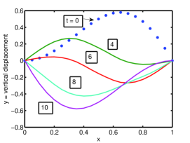
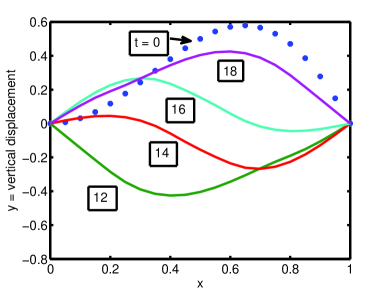
For $n\gg 1$, $a_{n}$ will approach $0$ like $(1/n)^{3},$ i.e., quite slowly. It is desirable to examine how many terms are needed in the numerical sum of Eq. (17) in order to get an accuracy of $4$ significant figures in $y.$ A good guess is that the sum of all terms not included in the sum

$$\sum_{n\max+1}^{\infty}a_{n}\cos(\omega_{n}t)\simeq-4\frac{L^{2}}{\pi^{2}}\sqrt{\frac{2}{L}}\int_{n\max+1}^{\infty}\frac{1}{n^{3}}\cos(\frac{c\pi}{L}t\ n)\ dn$$ (18)

should be less than $y_{\max}\times 10^{-4}.$ The integral in Eq. (18) is smaller than $\int_{n\max+1}^{\infty}(1/n)^{3}dn=(n_{\max}+1)^{-2}/2$ (since the $\cos$ term produces cancellations), and one obtains the estimate

$$|\sum_{n\max+1}^{\infty}a_{n}\cos(\omega_{n}t)|\ <2\frac{L^{2}}{\pi^{2}}\sqrt{\frac{2}{L}}(n\max+1)^{-2}$$ (19)

With $nmax=50$ the right hand side of Eq. (19) is $\simeq 10^{-4}.$ A numerical evaluation of the difference $|y^{(50)}(x,0)-f(x)|\$is less than$\ 10^{-5},$ which confirms that with $n\max=50$ the accuracy expected for $y^{(50)}(x,t)$ is better than $1:10^{4}.$

II.2 The inhomogeneous string by means of a Fourier series expansion

An approximate solution to Eq. (5) for $\psi_{n}$ is to expand it in terms of the Fourier sine waves given by Eq. (12), since these functions obey the same boundary conditions as the $\psi_{n}^{\prime}s.$ The approximation consists in truncating that expansion at an upper limit $\ell\max=N,$ and also drop the sub- and -superscript $(n)$ for the time being

$$\psi^{(N)}(x)=\sum_{\ell^{\prime}=1}^{N}d_{\ell^{\prime}}\phi_{\ell^{\prime}}(x).$$ (20)

Inserting expansion (20) into Eq. (5), remembering that $d^{2}\phi_{\ell}(x)/dt^{2}=-k_{\ell}^{2}\phi_{\ell}(x)$, multiplying Eq. (5) by a particular function $\phi_{\ell}(x)$, integrating both sides of the equation over $dx$ from $x=0$ to $x=L,$ and using the orthonormality of the functions $\phi_{\ell}(x),$ one obtains

$$-k_{\ell}^{2}\ d_{\ell}+\Lambda\sum_{\ell^{\prime}=1}^{N}R_{\ell,\ell^{\prime}}d_{\ell^{\prime}}=0$$ (21)

where

$$R_{\ell,\ell^{\prime}}=\int_{0}^{L}\phi_{\ell}(x)R(x)\phi_{\ell^{\prime}}(x)\ dx$$ (22)

are the matrix elements of the function $R$ over the basis functions $\phi_{\ell}.$ This equation (21) can also be written in matrix form, where

$$\begin{pmatrix}k_{1}^{2}&&&&\\ &k_{2}^{2}&&&\\ &&k_{3}^{2}&&\\ &&&\ddots&\\ &&&&k_{N}^{2}\end{pmatrix}\begin{pmatrix}d_{1}\\ d_{2}\\ d_{3}\\ \vdots\\ d_{N}\end{pmatrix}=\Lambda\begin{pmatrix}R_{1,1}&R_{1,2}&R_{1,3}&\cdots&R_{1,N}\\ R_{2,1}&R_{2,2}&R_{2,3}&\cdots&R_{2,N}\\ R_{3,1}&R_{3,2}&R_{3,3}&\cdots&R_{3,N}\\ \vdots&\vdots&\vdots&\ddots&\vdots\\ R_{N,1}&R_{N,2}&R_{N,3}&\cdots&R_{N,N}\end{pmatrix}\begin{pmatrix}d_{1}\\ d_{2}\\ d_{3}\\ \vdots\\ d_{N}\end{pmatrix},$$ (23)

or more succinctly

$$\mathbf{k}^{2}\vec{d}=\Lambda\ \mathbf{R}\vec{d}\mathbf{,}$$ (24)

where bold letters indicate matrices, and a vector quantity indicates a $(N\times 1)$ column. Since all the $k_{\ell}$’s are positive, the matrix $\mathbf{k}^{-1}$ can be defined as

$$\mathbf{k}^{-1}=\begin{pmatrix}k_{1}^{-1}&&&&\\ &k_{2}^{-1}&&&\\ &&k_{3}^{-1}&&\\ &&&\ddots&\\ &&&&k_{N}^{-1}\end{pmatrix}$$ (25)

and one can transform Eq. (24) into

$$\mathbf{M}_{fourier}\mathbf{\ }\vec{u}_{n}\mathbf{=}\frac{1}{\Lambda_{s}}\vec{u}_{n};~{}~{}~{}n=1,2,...N$$ (26)

where

$$\mathbf{M}_{fourier}\mathbf{=k}^{-1}\mathbf{R\ k}^{-1}$$ (27)

and

$$\vec{u}_{n}\ \mathbf{=k\ }\vec{d}_{n}\ \mathbf{.}$$ (28)

While Eq. (24) is a generalized eigenvalue equation, Eq. (26) is a simple eigenvalue equation. The vectors $\vec{u}_{n}$ are the $N$ eigenvectors of the  $N\times N$ matrix $\mathbf{M}_{fourier}$, and $1/\Lambda_{n}$ are the eigenvalues. Furthermore, since $\mathbf{R}$ is a symmetric matrix, $\mathbf{M}_{fourier}$ is also symmetric. The eigenvectors of a symmetric matrix are orthogonal to each other, i.e. $(\vec{u}_{n})^{T}\cdot\vec{u}_{m}=\delta_{n,m}.$ Here $T$ indicates transposition. However the vectors $\vec{d}_{n}$ are not orthogonal to each other, since $(\vec{d}_{n})^{T}\cdot\vec{d}_{m}=(\vec{u}_{n})^{T}\mathbf{k}^{-2}\vec{u}_{m}.$

In summary, the procedure is as follows

1. Choose an upper truncation limit $N$ of the sum (20);

2. Calculate the matrix elements $R_{\ell,\ell^{\prime}}$ so as to obtain the $N\times N$ matrix $\mathbf{R}$

3. Construct the matrix $\mathbf{M}_{fourier}$ from Eq. (27), and find the eigenvalues $(1/\Lambda_{n})$ and eigenvectors $\vec{u}_{n}$, $n=1,2,..N,$ by using the MATLAB eigenvalue command $[\mathbf{V},\mathbf{D}]=eig(\mathbf{M}).$ The output $\mathbf{D}$ is a diagonal matrix of the eigenvalues and $\mathbf{V}$ is a full matrix whose columns are the corresponding eigenvectors so that $\mathbf{M}\ast\mathbf{V}$ = $\mathbf{V}\ast\mathbf{D}$. For example $\vec{u}_{n}=\mathbf{V}(:,n)$

4. If $\vec{\Phi}(x)$ is the column vector of the $N$ basis functions $\phi_{\ell}(x)$, then $\psi(x)$ can be written as (the superscript $(N)$ is dropped now)

$$\psi_{n}(x)=(\vec{u}_{n})^{T}\mathbf{k}^{-1}\cdot\vec{\Phi}(x).$$ (29)

5. In view of Eq. (29) the coefficients $a_{n}=$and $b_{n}$ $=<g$ $\psi_{n}>$ can be written as

$$a_{n} =<f\psi_{n}>\ =(\vec{u}_{n})^{T}\mathbf{k}^{-1}\cdot<f\ \vec{\Phi}(x)>$$ (30)

$$b_{n} =<g\psi_{n}>\ =(\vec{u}_{n})^{T}\mathbf{k}^{-1}\cdot<g\ \vec{\Phi}(x)>$$ (31)

where $\langle f\ \vec{\Phi}(x)\rangle$ is the column vector of the integrals $\langle f\ \phi_{\ell}\rangle=\int_{0}^{L}f(x)\phi_{\ell}(x)dx,$ $\ell=1,2,..N.$

6. The final expression for $y(x,t)$ can be obtained by first obtaining the coefficients $e_{n}$

$$e_{n}(t)=(\vec{u}_{n})^{T}\mathbf{k}^{-1}\left[\langle f\ \vec{\Phi}(x)\rangle\cos(w_{n}t)+\langle g\ \vec{\Phi}(x)\rangle\frac{1}{w_{n}}\sin(w_{n}t)\right],$$ (32)

and then performing the sum

$$y(x,t)=\sum_{n=1}^{N}e_{n}(t)\psi_{n}(x)=\vec{e}^{\ T}\cdot\vec{\Psi}.$$ (33)

In the above, $\vec{e}$ is the column vector of all $e_{n}$’s, and $\vec{\Psi}$ is the column vector of all $\psi_{n}$’s. In the present discussion we limit ourselves to calculating the eigenvalues $\Lambda_{n}.$

Assuming that the mass per unit length changes with distance $x$ from the left end of the string as

$$R(x)=1+2x^{2},$$ (34)

and $c,$ $f(x)$ and $g(x)$ are the same as for the homogeneous string case,

$$L=1m,\ c=800\ m/s,\ f(x)=x\sin[(\pi/L)x],\ g(x)=0.$$ (35)

then the integrals (22) for the matrix elements $R_{\ell,\ell^{\prime}}$ can be obtained analytically with the result

$$R_{\ell,\ell^{\prime}} =2\ast 2\left(\frac{L}{\pi}\right)^{2}(-1)^{\ell+\ell^{\prime}}\left[\frac{1}{(\ell-\ell^{\prime})^{2}}-\frac{1}{(\ell+\ell^{\prime})^{2}}\right],\ \ \ell\neq\ell^{\prime}$$ (36)

$$R_{\ell,\ell} =1+2\ L^{2}\left[\frac{1}{3}-\frac{2}{(2\pi\ell)^{2}}\right],\ \ \ \ell=\ell^{\prime}.$$ (37)

The increase of $R$ with $x$ can be simply visualized with the choice (34). More realistic situations, such as the distribution of masses on a bridge, can be envisaged for future applications.

The numerical construction of the matrices $\mathbf{R}$ and $\mathbf{M}_{fourier}$ is accomplished in the MATLAB program $string\_fourier.m$ which in turn calls the function $inh\_str\_M.m$, using the input values

$$L=1m,~{}~{}c=800\ m/s,\$$ (38)

The truncation value $N$ of the sum Eq. (20) is set equal to either $30$ or $60$, and the corresponding dimension of the matrices $\mathbf{M}_{fourier}$ or $\mathbf{R}$ is $N\times N.$ These values are chosen so as to examine the sensitivity of the eigenvalues to the size of the matrix $\mathbf{M}_{fourier}\mathbf{.}$

The results for the eigenvalues $\Lambda_{n}$ are shown in Fig. (3)

Figure 3: The eigenvalues of the matrix $M_{fourier},$ defined in Eq.(27).  The quantity $N$ indicates the truncation value of the sum in Eq. (20), that expands the string displacement eigenfunction $\psi_{n}(x)$ into the Fourier functions $\phi_{\ell}(x)$. The dimension of the matrix $M_{fourier}$ is $N\times N$.

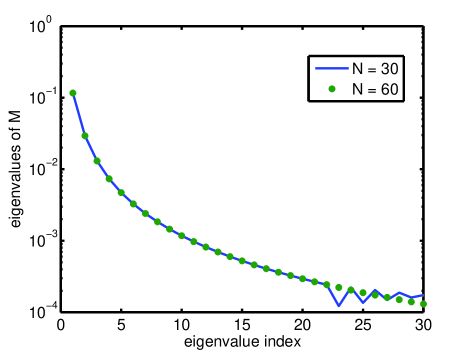
and the corresponding frequencies are shown in Fig. (4). The frequencies for the homogeneous string, i.e., for $R(x)=1$, are shown by the open circles in Fig. (4). Since the inhomogeneous string is more dense at large values of $x$ than the homogeneous one, the corresponding eigenfrequencies are correspondingly smaller. It is noteworthy that the eigenfrequencies of the inhomogeneous string nearly fall on a straight line, which means that the frequencies are nearly equispaced, i.e., they nearly follow the same harmonic relationship as the ones for the homogeneous string. The physical explanation for this property has not been investigated here, but could be connected to the fact that the waves for the high indices have more nodes than for the low indices, and hence lead to better averaging in a variational procedure.

Figure 4: The frequencies in units of radians/sec of the vibration of the inhomogeneous string, compared with the frequencies of the corresponding homogeneous string. The higher frequencies become inaccurate when the dimension of the matrix $M_{fourier}$ is too small.

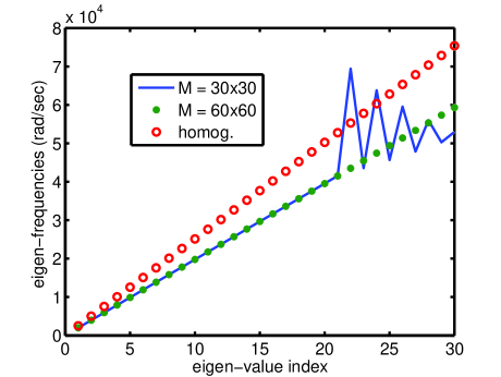
Near the fundamental frequency slight deviations from harmonicity do occur, as illustrated in Fig. (5).

Figure 5: The deviation from harmonicity as a function of the eigenfrequency index, for two different inhomogeneities. This deviation is defined in terms of the difference between two neighboring frequencies $d(n)=[w(n)-w(n-1)]$ as $\{d(n+1)/d(n)-1\}\ast 100.$ The inhomogeneity is given by $R(x)=1+F_{0}\ x^{2}$ with $F_{0}$ either $2~{}$or$~{}4.$

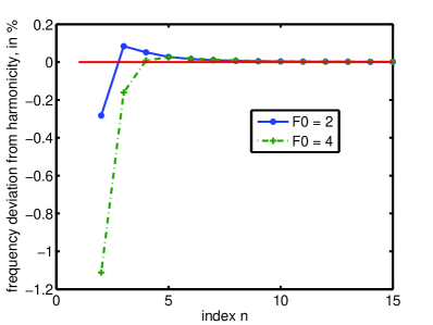
However, small deviations from harmonicity will also be caused by other effects such as the stiffness of the string.

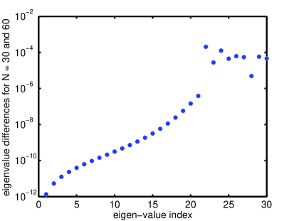
Figures (3) and (4) show that for the truncation value $N$ of $30$, the eigenvalues become unreliable for $n\geq 22$. This is a general property of the high-n eigenvalues of a matrix, which however can be overcome by using the iterative method described further on. The table 1 and Fig. (6) give a quantitative illustration of the dependence of the eigenvalue on the truncation value $N$ by the comparison of two eigenvalues for the same $n$ of the matrix $\mathbf{M}_{fourier}(30\times 30)$ with those of $\mathbf{M}_{fourier}(60\times 60)$.

n	$\mathbf{N=30}$	$\mathbf{N=60}$
1	1.614775590198150e-001	1.6147755902115e-001
20	4.092e-004	4.0933853097811e-004

Table 1: Eigenvalues of the matrix M for two different dimensions N x N

Figure 6: The dependence of the eigenvalues of the matrix $M_{fourier}$ on the dimension $N\times N$ of the matrix. The $y-$axis shows the absolute value of the difference between two sets of eigenvalues, one for $N=30,$ the other for $N=60$. Some numerical values are given in Table 1.

III
Spectral expansions into Chebyshev Polynomials

First some basic properties of Chebyshev polynomials will be described, then the Curtis-Clenshaw method for expanding functions in terms of these polynomials will be presented, with special emphasis on the errors associated with the truncation of the expansion, and finally the application to solving integral equations will be presented.

III.1 Properties of Chebyshev Polynomials

Chebyshev Polynomials $T_{v}(x)$ provide a very useful set of basis functions for expansion purposes RUDIN , LUKE . A short review of the main properties needed for the present application is presented below. The variable $x$ is contained in the interval $-1\rightarrow+1$, and is related to an angle $\theta$ by $x=\cos\theta$. This shows that the $x^{\prime}s$ are projections on the $x-$axis of the tip of a radius vector of unit length that describes a semi-circle as $\theta$ goes from $0$ to $\pi$. In terms of the $x-$variable the $T_{n}$’s are given by

$$\begin{array}[b]{c}T_{0}=1\\ T_{1}=x\\ T_{2}=2x^{2}-1\\ T_{n+1}=2xT_{n}-T_{n-1}\end{array}$$ (39)

In terms of the $\theta$ variable they are given by

$$T_{n}=\cos(n\ \theta);~{}~{}~{}0\leq\theta\leq\pi.$$ (40)

It is clear from Eq. (40) that $-1\leq T_{n}(x)\leq 1$, and that the larger the index $n$, the more zeros these polynomials have. The $T_{n}^{\prime}s$ are orthogonal to each other with the weight function $(1-x^{2})^{-1/2}.$ The integral $\mathcal{I}$

$$\mathcal{I}_{n,m}\mathcal{=}\int_{-1}^{+1}T_{n}(x)\ T_{m}(x)\ (1-x^{2})^{-1/2}\ dx=\int_{0}^{\pi}\ \cos(n\theta)\ \cos(m\theta)\ d\theta$$ (41)

has the value $0$ if $n\neq m$, and the values $\pi/2$ if $n=m\neq 0$ and $\pi$ if $n=m=0.$ A plot of $T_{v}(x)$ for $v=0,1,2,$ and $3$ is shown in Fig. (7), which also illustrates that for equispaced values of $\theta$ the corresponding values of $x$ are not equispaced.

Figure 7: Chebyshev Polynomials for indices $v=0,\ 1,2,$ and $3$. They are calculated from $T_{v}(x)=\cos(v\ast\theta),$ for the equispaced angles $\theta.$

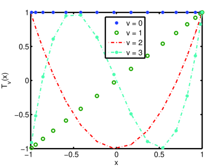
The values of $x,$ denoted as $\xi_{i},$ for which a particular $T_{n}=0,$ are also not equispaced. As can be seen from Eq. (40) the zeros $\xi_{i}$ of $T_{N+1}(x)$ with $i=0,1,2,..N$  are given by

$$\xi_{i}=\cos\left[\frac{(2\ i+1)}{2N+2}\pi\right]~{}\ i=0,1,2,..N.$$ (42)

III.2 The Expansion Method

Given a function $f(r)$, defined in the interval $[a,b],$ in order to expand it into Chebyshev polynomials, the first step is to transform the variable $r$ to a new variable $x$ defined in the interval $[-1,+1].$ This can be achieved by means of the linear transformation

$$r=\alpha\ x+\beta,$$ (43)

with $\alpha=(b-a)/2$ and $\beta=(b+a)/2.$ In terms of the $x-$variable one obtains the function $\bar{f}(x)=f(r),$ and the desired (truncated) expansion is

$$\bar{f}^{(N)}(x)=\sum_{n=0}^{N}\ a_{n}\ T_{n}(x).$$ (44)

The conventional method of obtaining the expansion coefficients $a_{n}$ is to multiply Eq. (44) on both sides by $T_{m}(x)/\sqrt{1-x^{2}}$, integrate over $x$ from $-1$ to $+1$, and use the orthogonality condition (41). A more computer friendly alternative was given by Clenshaw and Curtis CC . It consists in writing Eq. (44) $N+1$ times for the zeros $\xi_{0},\xi_{1},...\xi_{N},$ of the first Chebyshev polynomial $T_{N+1}$ not included in the sum (44), and thus obtain $N+1$ linear equations for the $N+1$ coefficients,

$$\bar{f}^{(N)}(\xi_{0}) =\sum_{n=0}^{N}\ a_{n}\ T_{n}(\xi_{0})$$

$$\bar{f}^{(N)}(\xi_{1}) =\sum_{n=0}^{N}\ a_{n}\ T_{n}(\xi_{1})..$$

$$\vdots$$

$$\bar{f}^{(N)}(\xi_{N}) =\sum_{n=0}^{N}\ a_{n}\ T_{n}(\xi_{N}).$$

which in matrix notation has the form

$$\begin{pmatrix}\bar{f}(\xi_{0})\\ \bar{f}(\xi_{1})\\ \vdots\\ \bar{f}(\xi_{N})\end{pmatrix}=C\ast\begin{pmatrix}a_{0}\\ a_{1}\\ \vdots\\ a_{n}\end{pmatrix}$$ (45)

where $C$ is known as the Discrete Cosine Transform. The points $\xi_{i}$ are denoted as ”support points” of the algorithm since the function $\bar{f}$ has to be known only at these points. The elements of the matrix $C$ are $C_{i,j}=T_{j}(\xi_{i}),$ and its columns are orthogonal to each other. After column normalization, one obtains an orthogonal matrix, and hence the inverse $C^{-1}$ can be easily obtained, without the need to invoke a numerical matrix inversion algorithm. The matrix $C^{-1}$ is denoted as $CM1$ in the MATLAB program $[C,CM1,z]=C\_CM1(N)$ available in Ref. PADRE . The row vector $z$ contains the values $\xi_{i}$ in descending order $i=N,\ N-1,\ ..0$. Inserting the values of $a_{i}$, obtained from Eq. (45) into Eq. (44), one obtains the value of the truncated function $\bar{f}^{(N)}(x)$ at any point in the interval $[-1,+1]$, and hence the procedure is an interpolation method DELOFF , SPECTRAL . Other cosine transforms also do exist, for example one based on the Fourier series expansion method. The method is computationally fast, in view of the advent of the FFT algorithms, however a comparison of the spectral method with this method is beyond the scope of the present article.

How good is approximation (44) to $\bar{f}(x)?$ If the function is differentiable $p$ times, then it can be shown ORZAG that

$$|\bar{f}^{(N)}(x)-\bar{f}(x)|\ \leq\frac{c}{p-1}\frac{1}{N^{p-1}}$$ (46)

where $c$ is a constant that depends on the $p$’s derivative of $\bar{f}.$ If the function $\bar{f}$ is infinitely differentiable, then $p=\infty$, and the error (46) decreases with $N$ faster than any power of $N.$ This is denoted as the supra-algebraic convergence of the approximation of $\bar{f}^{(N)}(x)$ to $\bar{f}(x)$, a property also denoted as ”spectral” expansion of $\bar{f}(x)$ in terms of Chebyshev polynomials ORZAG , DELOFF .

According to Luke LUKE , Theorem 2 in Chapter XI, section 11.7

$$|\bar{f}^{(N)}(x)-\bar{f}(x)|\ \simeq a_{N+1}T_{N+1}(x)\left[1+2x\ a_{N+1}/a_{N+2}\right]$$ (47)

In practice,

$$|\bar{f}^{(N)}(x)-\bar{f}(x)|\ \leq\ |a_{N+1}|$$ (48)

This property enables one to pre-assign an accuracy requirement $tol$ for the expansion (44). Either, for a given value of $N,$ the size of the partition of $r$ within which the function $f(r)$ is expanded can be determined, or, for a given size of the partition, the value of $N$ can be determined, such that the sum of the absolute values of the three last expansion coefficients $a_{N-2},\ a_{N-1}$ and $a_{N}$ is less than the value of $tol.$

An example will now be given that shows that, if the function $f$ is not infinitely differentiable, then the corresponding Chebyshev expansion converges correspondingly slowly. The two functions to be expanded are

$$f_{1}(r)=r^{1/2}\sin(r)$$ (49)

$$f_{2}(r)=r\ \sin(r)$$ (50)

in the interval $0\leq r\leq\pi.$ While $f_{2}$ is infinitely differentiable, all the derivatives of the function $f_{1}$ are singular at $r=0.$ The results for the Chebyshev expansions for the functions $f_{1}$ and $f_{2}$ using the Clenshaw-Curtis method are displayed in Fig. (8).

Figure 8: The Chebyshev expansion coefficients as a function of the index $v$, for the functions $f_{1}$ and $f_{2}$ defined in Eqs. (49) and (50). Since the derivatives of the function $f_{1}$ have a singularity at the origin, the Chebyshev expansion converges more slowly than that of $f_{2}$, which has an infinite number of non-singular derivatives.

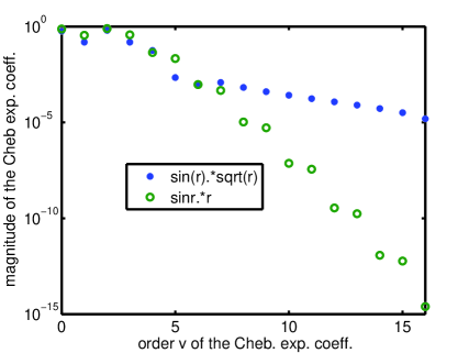
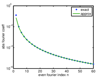
An expansion into a Fourier series of the function $f_{2}(r)=r\sin(\pi r)$ for $[0\leq r\leq 1]$ is also carried out for comparison with the expansion into Chebyshev polynomials. One finds that all Fourier coefficients $a_{n}$ with $n=1,2..$ defined in Eqs. (LABEL:9-11) through (16) for $L=1,$ vanish for $n$ odd, with the exception for $n=1$. For $n\gg 1$, $a_{n}$ will approach $0$ like $-4\sqrt{\frac{2}{\pi}}(1/n)^{3},$ i.e., quite slowly. The absolute value of this result is shown in Fig.(9). By comparison with Fig.(8) one sees that the Fourier expansion coefficients decrease with the index $n$ much more slowly than the Chebyshev expansion coefficients.

Figure 9: The Fourier expansion coefficients of the function $f(x)=x\sin(\pi\ x)$ in the interval $[0,1]$ in terms of the basis functions $\sqrt{\pi}\sin(n\pi\ x).$ The analytic result, given by Eqs. (15) and (16) with $L=1$, is shown by the symbols $\ast$. For odd values of $n\neq 1$ they are zero. The solid line represents an approximation to $|$$a_{n}|\simeq 4\sqrt{\frac{2}{\pi}}(1/n)^{3}$.

III.3 Integrals based on spectral expansions.

Given a function $f(r)$, defined in an interval $a\leq r\leq b$, it is the purpose of this sub-section to numerically obtain a spectral approximation to the indefinite integral of this function

$$\mathfrak{I(}r\mathfrak{)}=\int_{a}^{r}f(r^{\prime})dr^{\prime}$$ (51)

As is done in Eq. (43) the function $f(r)$ is transformed from the variable $r$ to the function $\bar{f}(x)$ for the variable $x\subset[-1,+1]$. Then the integral (51) becomes

$$\mathfrak{I(}r\mathfrak{)=}\frac{\mathfrak{(}b-a)}{2}I_{L}(x)$$ (52)

where

$$I_{L}(x)=\int_{-1}^{x}\bar{f}(x^{\prime})dx^{\prime}.$$ (53)

It is desired to obtain the spectral expansion of the approximation to $I_{L}(x)$

$$I_{L}^{(N)}(x)=\sum_{n=0}^{N}\ b_{n}\ T_{n}(x)$$ (54)

where it is assumed that $\bar{f}(x)$ has been expanded in a series of Chebyshev polynomials, as given by Eq. (44). In view of the integral properties of Chebyshev polynomials, the coefficients $b_{n}$ can be expressed in terms of the expansion coefficients $a_{n}$ of $\bar{f}(x),$

$$\begin{pmatrix}b_{0}\\ b_{1}\\ \vdots\\ b_{N}\end{pmatrix}=S_{L}\begin{pmatrix}a_{0}\\ a_{1}\\ \vdots\\ a_{N}\end{pmatrix}$$ (55)

by means of the matrix $S_{L}$ CC , without loss of accuracy. For the integral

$$I_{R}(x)=\int_{x}^{1}\bar{f}(x^{\prime})dx^{\prime}$$ (56)

an expression similar to (55) exists, with the matrix $S_{L}$ replaced by $S_{R}.$ Numerical expressions for the matrices $S_{L}$ and $S_{R}$ exist in the literature IEM , DELOFF-INT and are also available from Ref. PADRE under the name $SL\_SR.$ In particular, by noting that $T_{n}(1)=1$ for all $n,$ an approximation to the definite integral $\mathfrak{I(}r_{2}\mathfrak{)}=\int_{a}^{b}f(r^{\prime})dr^{\prime}$ is given by

$$\mathfrak{I}^{(N)}\mathfrak{(}b\mathfrak{)=}\frac{\mathfrak{(}a-b)}{2}\sum_{n=0}^{N}b_{n}$$ (57)

with an error comparable to Eq. (48), of the order of $|b_{N+1}|.$ The above form of the definite integral (57) is denoted below as Gauss-Chebyshev quadrature. The existence of Eq. (55) makes the expansion into Chebyshev polynomials very suitable for the numerical solution of integral equations, as will be seen below.

As an example, the integrals

$$\mathfrak{I}_{1} =\int_{0}^{\pi}r^{1/2}\ \sin(r)\ dr$$ (58)

$$\mathfrak{I}_{2} =\int_{0}^{\pi}r\ \sin(r)\ dr$$ (59)

are evaluated below by using Eq. (57). For comparison purposes $\mathfrak{I}_{1}$ was also evaluated using the MATLAB integration function $quad(@myfun,0,\pi,acc),$ where $acc$ denotes the precision to within which the quadrature result is given. The results  are shown in the last line of table 2

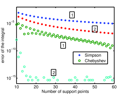
If one uses an expansion of the integrand $f(r)=\sin(r)\ast r^{1/2}$ into a set of Chebyshev polynomials, and uses the integral properties of these polynomials by means of the function $[SL,SR]=SL\_SR(N)$, then for $60$ support points $N$ one gets an accuracy of $1:10^{-9},$ but the convergence with $N$ is slow, as is also the case for the expansion coefficients of $f_{1}$. The values of $\mathfrak{I}_{1}$ for two values of $N$ are shown in Table 2 below

$Cheb.,\ N=58$	$2.43532116647$
$Cheb.,\ N=59$	$2.43532116702$
$quad,\ acc=10^{-11}$	$2.4353211641\mathbf{7}$

Table 2: Integral (58) obtained with the Chebyshev method, for benchmark purposes

. If, on the other hand, one instead uses for the integrand the analytic function $f_{2}(r)=\sin(r)\ast r,$ then the corresponding integral converges with $N$ much faster, reaching machine accuracy for $N=18.$ These convergence properties are displayed in Fig. (10), where a comparison of the convergence using Simpson’s quadrature method is also shown.

Figure 10: Comparison of the convergence properties of the Gauss-Chebyshev and the Simpson integration procedures as a function of the number of support points. The labels $1$ or $2$ denote the integrals $I_{1}=\int_{0}^{\pi}\sin(r)\ r^{1/2}\ dr$ or  $I_{2}=\int_{0}^{\pi}\sin(r)\ r\ dr,$ respectively.

IV The integral equation for the inhomogeneous string.

In the previous discussion the Sturm-Liouville functions $\psi_{n}(r),$ solutions of Eq. (5), were obtained by expanding them into a set of Fourier functions $\phi_{\ell}(r),$ and obtaining the eigenfunctions and eigenvalues of the matrix $M_{fourier}.$ This matrix consisted of overlap integrals of the inhomogeneity function $R(x)$ with the basis functions $\phi_{\ell}(x).$ In the present section three major innovations are introduced: a) we transform the differential equation (5) into an integral equation, since the numerical solution of the latter is more stable than that of the former, b) we replace the need to do overlap integrals by the Curtis Clenshaw method, Eq. (45), of obtaining the expansion coefficients, and c) the basis functions are the Chebyshev polynomials for which the expansion series converges much faster than for the Fourier expansions.

The integral equation that is equivalent to the differential equation (5) is

$$\frac{1}{\Lambda}\psi(r)=-\int_{0}^{L}\mathcal{G}(r,r^{\prime})\ R(r^{\prime})\ \psi(r^{\prime})dr^{\prime}$$ (60)

where the Green’s function $\mathcal{G}(r,r^{\prime})$ is given by

$$\mathcal{G}(r,r^{\prime}) =-\frac{1}{L}F(r)G(r^{\prime})\text{ for }r<r^{\prime}$$ (61)

$$\mathcal{G}(r,r^{\prime}) =-\frac{1}{L}F(r^{\prime})G(r)\text{ for }r>r^{\prime}$$

and where

$$F(r)=r;~{}~{}G(r)=(L-r).$$ (62)

Both functions $F$ and $G$ obey the equation $d^{2}F/dr^{2}=0,$ $d^{2}G/dr^{2}=0$ and they are linearly independent of each other. Because of the separable nature of $\mathcal{G}$ the integral on the right hand side of Eq. (60) can be written as

$$\int_{0}^{L}\mathcal{G}(r,r^{\prime})\ R(r^{\prime})\ \psi(r^{\prime})dr^{\prime} =-\frac{1}{L}G(r)\int_{0}^{r}F(r^{\prime})R(r^{\prime})\ \psi(r^{\prime})dr^{\prime}$$

$$-\frac{1}{L}F(r)\int_{r}^{L}G(r^{\prime})R(r^{\prime})\ \psi(r^{\prime})dr^{\prime}$$ (63)

In view of the fact that $F$ vanishes at $r=0$ and $G$ vanishes at $r=L,$ and hence $\int_{0}^{L}\mathcal{G}(r,r^{\prime})\ R(r^{\prime})\ \psi(r^{\prime})dr^{\prime}$ vanishes for both $r=0$ and $r=L,$ the functions $\psi$ satisfy the boundary conditions. A proof that $\psi(r)$ defined by Eq. (60) satisfies Eq. (5) can be obtained by carrying out the second derivative in $r$ of Eq. (63).

The numerical solution of Eq. (60) is accomplished by first changing the variable $r$, contained in the interval $[0,L]$, into the variable $x$, contained in the interval $[-1,+1],$ which results in the transformed functions $\bar{\psi}(x)$, $\mathcal{\bar{G}}(x,x^{\prime})$, and $\bar{R}(x^{\prime}).$ Expanding the unknown solution $\bar{\psi}(x)$ into Chebyshev polynomials

$$\bar{\psi}(x)=\sum_{n=0}^{N}\ a_{n}T_{n}(x),$$ (64)

as was done in Eq. (44), then Eq. (60) leads to a matrix equation in the coefficients $a_{n}$, as will now be shown. The coefficients $a_{n}$ can be placed into a column vector

$$\vec{a}=[a_{0},a_{1},..,a_{N}]^{T},$$ (65)

where $T$ means transposition. The values of $\bar{\psi}(\xi_{i})$ at the support points $\xi_{i}$, which are the zeros of $T_{N+1},$ can also be expressed as a column vector

$$\vec{\psi}=[\bar{\psi}(\xi_{0}),\ \bar{\psi}(\xi_{1}),\ ...\bar{\psi}(\xi_{N})]^{T},$$ (66)

and the relation between $\vec{a}$ and $\vec{\psi},$ already given in Eq. (45), is

$$\vec{a}=\mathbf{C}^{-1}\ \vec{\psi},~{}~{}\vec{\psi}=\mathbf{C\ }\vec{a}$$ (67)

Another important relation concerns the integrals

$$\Phi_{L}(x)=\int_{-1}^{x}\phi(x^{\prime})\ dx^{\prime}\text{ and }\Phi_{R}(x)=\int_{x}^{1}\phi(x^{\prime})\ dx^{\prime},$$ (68)

where $\phi$ is a function defined in the interval $[-1,1]$, and the corresponding expansion coefficients $\alpha_{n}$ are given by $\vec{\alpha}=\mathbf{C}^{-1}\ \vec{\phi}$. If $\Phi_{L,R}(x)$ is expanded into Chebyshev polynomials

$$\Phi_{L}(x)=\sum_{n=0}^{n=N}\ \beta_{n}^{(L)}T_{n}(x)\text{ and~{} }\Phi_{R}(x)=\sum_{n=0}^{n=N}\ \beta_{n}^{(R)}T_{n}(x)$$ (69)

then the expansion coefficients $\beta$ can be expressed in terms of the expansion coefficients $\alpha$ of $\phi$ by means of the matrices $\mathbf{S}_{L}$ and $\mathbf{S}_{R},$ described near Eq. (55),

$$\vec{\beta}^{(L)}=\mathbf{S}_{L}\vec{\alpha}\text{ and }\vec{\beta}^{(R)}=\mathbf{S}_{R}\vec{\alpha}\text{.}$$ (70)

The matrices $\mathbf{C,\ C}^{-1},\ \mathbf{S}_{L}$ and $\mathbf{S}_{R}$ can either be obtained from Ref. PADRE or can be found in Ref.IEM . Making use of Eqs. (67) and (70) one can write the Chebyshev expansion of the right and left hand sides of Eq. (60) as

$$\frac{1}{\Lambda}\vec{a}=\mathbf{M}_{IEM}\ \vec{a}$$ (71)

where

$$\mathbf{M}_{IEM}=\frac{1}{2}\ast\mathbf{C}^{-1}\ast M3\ast DR\ast\mathbf{C}.$$ (72)

In the above the factor $1/2$, comes from the transformation of coordinates from $r$ to $x,$ and where the term $L$ was cancelled by the $(1/L)$ in Eq. (63); $DR$ is the diagonal matrix that contains the values of $R(\xi_{i})$ along the main diagonal, and $M_{3}$ is given by

$$\mathbf{M}_{3}=DG\ast\mathbf{C}\ast S_{L}\ast\mathbf{C}^{-1}\ast DF+DF\ast\mathbf{C}\ast S_{R}\ast\mathbf{C}^{-1}\ast DG.$$ (73)

The first (second) term in Eq. (73) represents the first (second) term in Eq. (63), $DF=diag(F)$ and $DG=diag(G)$ represent the diagonal matrices having the values of $F(\xi_{i})$ and $G(\xi_{i})$ along the main diagonal, the $\xi_{i}$ being the $N+1$ support points described near Eq. (45).

The explanation for Eq. (71) is as follows: the matrix $\mathbf{M}_{IEM}$ in Eq. (72) is applied to the column vector $\vec{a},$ the $\mathbf{C}$ in (72) transforms the $\vec{a}$ into the vector $\vec{\psi},$ the factor $DR$ together with the factor $DG$ in (73) transforms $\vec{\psi}$ into $\vec{G}\otimes\vec{R}\otimes\vec{\psi}$ (the symbol $\otimes$ means that in $\vec{G}\otimes\vec{R}$ each element of the vector $\vec{G}$ is multiplied by the corresponding element of the vector $\vec{R}$, and a new vector of the same length is produced), the additional factor $\mathbf{C}^{-1}$ produces the expansion coefficients of $\vec{G}\otimes\vec{R}\otimes\vec{\psi}$, the matrix $S_{L}$ or $S_{R}$ transforms these expansion coefficients to the expansion coefficients of the respective indefinite integrals, etc.

IV.1 Results

After choosing a certain value for the number $N_{IEM}+1$ of Chebyshev coefficients a numerical value of the ($N_{IEM}+1)\times(N_{IEM}+1)$ matrix (72) is obtained, from which the eigenvalues $(1/\Lambda_{n})$, $n=1,2,...N_{IEM}+1$ can be calculated.  The MATLAB computing times for the Fourier method for $N_{fourier}=30$ and $60$ combined using the analytic expressions for the integrals needed to obtain the elements of the matrix $\mathbf{R}$ is $0.91s$, while the computing time for the $IEM$ matrix method for all three $N_{IEM}=30,\ 60,$ and $90$ values combined is $0.75s.$ Hence the IEM method is comparable in complexity to the Fourier expansion method, provided that the overlap integrals (22) are known analytically. However, a disadvantage of the $IEM$ for this application is that some eigenvalues are spurious. Their occurrence can be recognized in that they change with the value of $N_{IEM},$ and do not coincide with the eigenvalues of $\mathbf{M}_{fourier}.$

The accuracy of these two matrix methods is illustrated in Fig. (11). It is based on the iterative method described below, used as an accuracy benchmark, since it gives an accuracy of $1:10^{11}$ for the eigenvalues regardless of the value of the eigenvalue index $n.$

Figure 11: Accuracy of the eigenvalues of $M_{fourier}$ and $M_{IEM}$ for various values of their dimension $N\times N.$ The value of $N$ is indicated in parenthesis in the legend. For the Fourier method, $N$ is the number of basis functions $\phi_{\ell}$ used to expand the Sturm-Liuoville eigenfunctions, and for the $IEM$, $N$ is the number of Chebyshev polynomials used in the expansion, which is also equal to the number of support points in the interval $[0,L].$ The accuracy of the matrix eigenvalues is obtained by comparison with a highly accurate result of $1$ part in $10^{11}$ obtained by an iterative method.

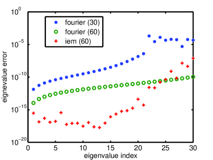
Figure (11) shows that the accuracy of the IEM matrix method is considerably higher than the Fourier matrix method for the low values of $n$, but it is not as monotonic as the latter. The figure also shows that the accuracy of both matrix methods depends sensitively on the dimension $N$ of their respective matrices $M$.

V The iterative method

This iterative method was introduced by Hartree HART in the 1950’s in order to calculate energy eigenvalues of the Schrödinger equation for atomic systems. The method was adapted to the use of the spectral expansion method ($IEM$) and applied to the energy eigenvalue of the very tenuously bound Helium-Helium dimer HEHE . The version described below for finding the eigenvalues that multiply the inhomogeneity function $R,$ with appropriate modifications is also suitable for finding the eigenfunctions for more general SL equations, such as the Schrödinger equation STURM . The method is as follows.

For a slightly wrong value $\Lambda_{1}$ of $\Lambda$ there is a slightly wrong function $\psi_{1}$ that obeys the equations

$$\frac{d^{2}\psi_{1}(r)}{dr^{2}}+\Lambda_{1}R(r)\ \psi_{1}(r)=0.$$ (74)

This function does not satisfy the boundary conditions at both $r=0$ and $r=L$ unless it has a discontinuity at some point $r_{I}$, contained in the interval $[0,L].$ To the left of $r_{I}$ the function $\psi_{1}$ that vanishes at $r=0$ is called $Y_{1}(r),$ and to the right of $r_{I}$ it is called $k\ast Z_{1}(r),$ and vanishes at $r=L.$ Here $\mathfrak{k}$ is a normalization factor chosen such that $Y_{1}(r_{I})=\mathfrak{k}$ $Z_{1}(r_{I}).$ Both these functions rigorously obey Eq. (74) in their respective intervals and are obtained by solving the integral equations

$$Y_{1}(r)=F(r)-\Lambda_{1}\int_{0}^{r_{I}}\mathcal{G}(r,r^{\prime})R(r^{\prime})Y_{1}(r^{\prime})dr^{\prime},~{}~{}0\leq r\leq r_{I}$$ (75)

and

$$Z_{1}(r)=G(r)-\Lambda_{1}\int_{r_{I}}^{L}\mathcal{G}(r,r^{\prime})R(r^{\prime})Z_{1}(r^{\prime})dr^{\prime},~{}~{}r_{I}\leq r\leq L.$$ (76)

These integral equations differ from Eq. (60), due to the presence of a driving term $F$ or $G$. However, since the second derivatives of these functions are zero, their presence does not prevent that $Y_{1}$ and $Z_{1}$ obey Eq. (74) in their respective domains.

The iteration from $\Lambda_{1}$ to a value closer to the true $\Lambda$ proceeds as follows. One multiplies Eq. (77)

$$\frac{d^{2}Y_{1}(r)}{dr^{2}}+\Lambda_{1}R(r)\ Y_{1}(r)=0,\ 0\leq r\leq r_{I}$$ (77)

with $\psi(r)$ and one multiplies Eq. (5) with $Y_{1}(r),$ subtracts one from the other, and integrates from $r=0$ to $r=r_{I}.$ One finds that $\int_{0}^{r_{I}}(Y_{1}^{\prime\prime}\psi-\psi^{\prime\prime}Y_{1})dr^{\prime}=$ $(Y_{1}^{\prime}\psi-\psi^{\prime}Y_{1})_{r_{I}}=(\Lambda-\Lambda_{1})\int_{0}^{r_{I}}Y_{1}\psi dr^{\prime}$. Here a prime denotes the derivative with respect to $r.$ A similar procedure applied to $Z_{1}$ in the interval $[r_{I},L]$ yields $-\mathfrak{k\ }(Z_{1}^{\prime}\psi-\psi^{\prime}Z_{1})_{r_{I}}=(\Lambda-\Lambda_{1})\int_{0}^{r_{I}}\mathfrak{k\ }Z_{1}\psi dr^{\prime}.$ Adding these two results and remembering that $\mathfrak{k}Z_{1}=Y_{1}$ for $r=r_{I}$, and dividing the result by $\psi(r_{I})\mathfrak{k}Z_{1}(r_{I})$ one obtains

$$\Lambda-\Lambda_{1}=\frac{(Y^{\prime}/Y-Z^{\prime}/Z)_{r_{I}}}{\frac{1}{(Y_{1}\psi)_{r_{I}}}\int_{0}^{r_{I}}Y_{1}R\psi dr^{\prime}+\frac{1}{(Z_{1}\psi)_{r_{I}}}\int_{r_{i}}^{L}Z_{1}R\psi dr^{\prime}}.$$ (78)

This result is still exact, but the exact function $\psi$ is not known. The iterative approximation occurs by replacing $\psi$ in the first integral in the denominator by $Y_{1}$, and by $\mathfrak{k\ }Z_{1}$ in the second integral, and by replacing $\psi(r_{I})$ in the denominators of each integral by either $Y_{1}(r_{I})$ or by $\mathfrak{k\ }Z_{1}(r_{I}).$ The final result is

$$\Lambda_{2}=\Lambda_{1}+\frac{(Y^{\prime}/Y-Z^{\prime}/Z)_{r_{I}}}{\frac{1}{Y_{1}^{2}(r_{I})}\int_{0}^{r_{I}}Y_{1}^{2}Rdr^{\prime}+\frac{1}{Z_{1}^{2}(r_{I})}\int_{r_{i}}^{L}Z_{1}^{2}Rdr^{\prime}}.$$ (79)

In the above, $\Lambda$ was replaced by $\Lambda_{2}$ as being a better approximation to $\Lambda$ than $\Lambda_{1},$ and the normalization factor $\mathfrak{k}$ has cancelled itself out. The iteration proceeds by replacing $\Lambda_{1}$ in the above equations by the new value $\Lambda_{2}.$

The derivatives in the numerator of Eq. (79) can be obtained without loss of accuracy by making use of the derivatives of Eqs. (75) and (76)

$$\ Y_{1}^{\prime}(r)=F^{\prime}(r)+\frac{\Lambda_{1}}{L}G^{\prime}(r)\int_{0}^{r}F(r^{\prime})R(r^{\prime})\ Y_{1}(r^{\prime})dr^{\prime}+\frac{\Lambda_{1}}{L}F^{\prime}(r)\int_{r}^{r_{I}}G(r^{\prime})R(r^{\prime})\ Y_{1}(r^{\prime})dr^{\prime}$$ (80)

and

$$Z_{1}^{\prime}(r)=G^{\prime}(r)+\frac{\Lambda_{1}}{L}G^{\prime}(r)\int_{r_{I}}^{r}F(r^{\prime})R(r^{\prime})\ Z_{1}(r^{\prime})dr^{\prime}+\frac{\Lambda_{1}}{L}F^{\prime}(r)\int_{r}^{L}G(r^{\prime})R(r^{\prime})\ Z_{1}(r^{\prime})dr^{\prime}$$ (81)

with the result at $r=r_{I}$

$$Y_{1}^{\prime}(r_{I})=1-\frac{\Lambda_{1}}{L}\int_{0}^{r_{I}}r^{\prime}R(r^{\prime})\ Y_{1}(r^{\prime})dr^{\prime}$$ (82)

and

$$Z_{1}^{\prime}(r_{I})=-1+\frac{\Lambda_{1}}{L}\int_{r_{I}}^{L}(L-r^{\prime})R(r^{\prime})\ Z_{1}(r^{\prime})dr^{\prime}$$ (83)

In the present formulation the dimensions of $\Lambda$ are $\ell^{-2},$ and the dimension of $F$, $G,$ $Y$ and $Z$ are $\ell,$ where $\ell$ represents a unit of length. As noted above, the derivatives with respect to $r$ of the functions $Y$ or $Z$ or $\psi$ are not obtained as the difference between two adjoining positions, but rather as the known derivatives of $F$ and $G$, together with integrals over $Y$ or $Z$ or $\psi$ according to Eqs. (80) and (81). In the $IEM$ formulation these integrals can be obtained with the same spectral precision as the calculation of the functions $Y$ or $Z$ or $\psi,$ CISE , hence there is no loss of accuracy either for the evaluation of Eq. (79), or for the calculation of $\Lambda,$ which can be set to $1:10^{11}$. However, it is important to start the iteration with a guessed value of $\Lambda$ that lies within the valley of convergence of Eq. (79). These initial values can be obtained, for example, from the eigenvalues of the matrix $\mathbf{M}_{fourier}$ described above, or from a method described in Ref. HEHE .

V.1 Results for the iterative method

Some of the values for $\Lambda_{n}$ obtained to an accuracy of $1:10^{11}$ by means of the iterative method described above are listed in Table 3, so as to serve as benchmark results for comparisons with future methods. The starting values $\Lambda_{1}$ for each $n$ are the results of the Fourier method described above with $N=60.$ The iterations were stopped when the change $\Lambda_{2}-\Lambda_{1}$ became less than $10^{-12}$ (usually three iterations were required), and $tol=10^{-11}.$

$\mathbf{n}$	$\mathbf{\Lambda}_{n}$	$\mathbf{n}$	$\mathbf{\Lambda}_{n}$
$1$	1.61477559021e-001	$26$	2.42220326385e-004
$2$	4.06257259855e-002	$27$	2.24611142229e-004
$3$	1.81281029690e-002	$28$	2.08854647313e-004
$4$	1.02131986136e-002	$29$	1.94699775697e-004
$5$	6.54130338213e-003	$30$	1.81936592475e-004

Table 3: Eigenvalues of Eq.(5) obtained iteratively with Eqs.(79)

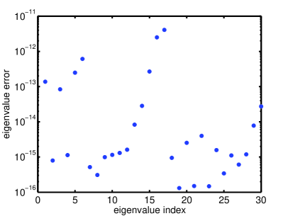
The error of the functions $Y$ and $Z$ is given, according to Eq. (48), by the size of the high order Chebyshev expansion parameters. For the $tol$ parameter of $10^{-11}$ their values stay below $10^{-11},$ as is shown in Fig. (12). Since there is no loss of accuracy in evaluating the various terms in Eq. (79), the error in the iterated eigenvalues $\Lambda$ is also given by Fig. (12). In order to achieve this type of error, the number $N$ of Chebyshev polynomials used for the spectral expansion of the functions $Y$ and $Z$ for the solution of their respective integral equations was increased adaptively by the computer program. It was found that for $n=1$, $N=16$; for $n=2$ to $6$, $N=24$; for $n=7$ to $23$, $N=24$; and for $n=18$ to $30$, $N=54$. This procedure of increasing $N$ is different from the procedure used in Ref. HEHE , where $N$ was kept constant and the number of partitions was increased adaptively. The latter method was required because of the long range ($3000$ units of length) of the $He-He$ wave functions.

Figure 12: The $y$-axis shows the absolute value of the mean square average of the three last Chebyshev coefficents  in the expansions of the functions $Y$ and $Z.$ As discussed in the text, the error of the eigenvalues $\Lambda$ is also given by the $y-$axis. The number $N$ of expansion Chebyshev polynomials was increased adaptively as the eigenvalue index $n$ increased. The ”jumps” in the values of these errors is due to the transition from one value of $N$ to a suddenly larger value, as is explained in the text.

VI Summary and conclusions

The main aim of this paper is to introduce the spectral expansion method for solving integral equations to the teaching community, with the hope that this method can be included in computational physics courses in the future. Such expansions converge rapidly with high precision, and complement the usual finite difference methods in common use today. The example used for the application of such a method is the analysis of the vibration of an inhomogeneous string in the separation of variables formalism. The spatial basis functions $\psi_{n}(r),$ $n=1,2,...,$ form a complete Sturm-Liouville set, the calculation of which is performed by means of three methods. In method $1$ the function $\psi$ is expanded into a basis set of sine waves, and the eigenfrequencies and expansion coefficients for each $\psi_{n}$ are the eigenvalues and eigenvectors of a matrix $\mathbf{M}_{fourier}.$ In method $2$ the differential equation for $\psi_{n}$ is transformed into an integral equation of the Lippmann Schwinger type, the unknown function is expanded into Chebyshev polynomials, and the expansion coefficients are again the eigenvectors of another matrix $\mathbf{M}_{IEM}.$ The comparison between these two methods illustrates the differences and advantages of each, especially their properties as a function of the size of the expansion basis. In method $3$, which has not been presented previously, the differential equation for the Sturm-Liouville eigenfunction is solved iteratively, and the auxiliary functions required for the iterations are obtained from the solutions of the corresponding integral equation. The advantage of method $3$ is that the precision of both the eigenfunction and the eigenvalue can be predetermined by specifying the value of a tolerance parameter, and further, no eigenvalue calculation of big matrices is required. In the present application the results of method $3$ were accurate to $1:10^{11}.$

The comparison between the accuracies of the various methods is illustrated extensively by means of appropriate graphs and tables. Applications of these methods to other problems, such as the solution of the Schrödinger equation, or the heat propagation equation, or diffusion equations in biology, are of course quite possible in spite of the present focus on the inhomogeneous string equation.

References

- (1) C. F. Gerald and P. O. Wheatley, Applied Numerical Analysis, 6th ed. (Addison-Wesley, Reading, Mass, 1999); S. Koonin, Computational Physics” (Benjamin-Cummings, 1985); Rubin H. Landau and M. J. P. Mejía, Computational physics : problem solving with computers (John Wiley & Sons, New York, c1997); P. L. DeVries, A first Course in Computational Physics (John Wiley and Sons, N. Y., 1994);
- (2) R. Chabaya and B. Sherwood, ”Computational physics in the introductory calculus-based course”, Am. J. Phys. 76, 307-313 (2008); D. M. Cook, ”Computation in undergraduate physics: The Lawrence approach”, Am. J. Phys. 76, 321-326 (2008); C. Rebbi, ”A project-oriented course in computational physics: Algorithms, parallel computing, and graphics”, Am. J. Phys. 76, 314-320 (2008) ; Harvey Gould, ”Computational physics and the undergraduate curriculum” Computer Physics Communications 127 6–10 (2000);
- (3) G. Rawitscher,I Koltracht, H. Dai, ; C. Ribetti, ”The vibrating string: a fertile topic for teaching scientific computing”, Computers in Physics, 10, 335-340 (1996);
- (4) R. A. Gonzales, J. Eisert, I Koltracht, M. Neumann and G. Rawitscher, ”Integral Equation Method for the Continuous Spectrum Radial Schrödinger Equation”, J. of Comput. Phys. 134, 134-149 (1997); R. A. Gonzales, S.-Y. Kang, I. Koltracht and G. Rawitscher, ”Integral Equation Method for Coupled Schrödinger Equations”, J. of Comput. Phys. 153, 160-202 (1999);
- (5) Rawitscher, G. and Koltracht, I., ”Description of an efficient Numerical Spectral Method for Solving the Schrödinger Equation”, Computing in. Sc. and Eng., 7, 58-66 (2005); G. Rawitscher, ”Applications of a Numerical Spectral Expansion Method to Problems in Physics; a Retrospective”, Operator Theory, Advances and Applications, 203, 409-426 (2009) (Birkäuser Verlag, Basel, Switzerland);
- (6) A. Palacios, T.N.A. Rescigno, C.W.McCurdy, ”Two-electron time-delay interference in atomic double ionization by attosecond pulses”, Phys. Rev. Lett., 103, 253001-4 (2009); W. Gloeckle, G. Rawitscher, ”Scheme for an accurate solution of Faddeev integral equations in configuration space”, Nucl. Phys. A 790, 282-5 (2007);
- (7) Hartree, D. R., ”The Calculation of Atomic Structures”, (John Wiley, 1955), p. 86;
- (8) Rawitscher, G. and I. Koltracht I., ”An economical method to calculate eigenvalues of the Schrödinger equation”, Eur. J. Phys. 27,1179-1192 (2006);
- (9) G. W. Recktenwald, Numerical Methods with MATLAB: Implementation and Application, (Prentice Hall, Upper Saddle River, New Jersey, 2000);
- (10) A digital library located at http://www.compadre.org/ucomp.
- (11) Lloyd N. Trefethen, Spectral Methods in MATLAB SIAM (Philadelphia, PA, 2000);
- (12) Mary L. Boas, Mathematical Methods in the Physical Sciences, 2nd ed. (John Wiley&Sons, 1983), Problem 24 on p. 540; D. A. McQuarrie, Mathematical Methods for Scientists and Engineers, (University Science Books, 2003), p 687 ff;
- (13) T. J. Rudin, The Chebyshev Polynomials, (John Wiley, 1974);
- (14) Y.L. Luke, Mathematical Functions and their Approximations (Academic Press, New York, 1975);
- (15) C. W. Clenshaw and A. R. Curtis, ” A method for numerical integration on an automatic computer”, Numerical Mathematics, 2, 197, (1960);
- (16) A. Deloff, ”Semi-spectral Chebyshev method in quantum mechanics”, Ann. of Phys. 322, 1373-1419 (2007);
- (17) D. Gottlieb and S. A. Orszag, Numerical Analysis of Spectral Methods: Theory and Applications, CBMS-NSF Regional Conference Series in Applied Mathematics, Vol 26 (SIAM , Philadelphia 1977);
- (18) A. Deloff, ”Gauss-Legendre and Chebyshev quadratures for singular integrals”, Computer Physics Communications, 179, 908-914 ( 2008);
- (19) G. Rawitscher, ”Positive energy Weinberg states for the solution of scattering problems”, Phys. Rev. C 25, 2196-2213, (1982);