The conflict triad dynamical system
Abstract
A dynamical model of the natural conflict triad is investigated. The conflict interacting substances of the triad are: some biological population, a living resource, and a negative factor (e.g., infection diseases). We suppose that each substance is multi-component. The main coexistence phases for substances are established: the equilibrium point (stable state), the local cyclic orbits (attractors), the global periodic oscillating trajectories, and the evolution close to chaotic. The bifurcation points and obvious thresholds between phases are exhibited in the computer simulations.
1 Institute of Mathematics, Tereshchenkivs’ka str. 3, Kyiv 01601 Ukraine E-mail: kosh@imath.kiev.ua
2 Institute of Mathematics, Tereshchenkivs’ka str. 3, Kyiv 01601 Ukraine E-mail: isamoil@imath.kiev.ua
AMS Subject Classifications: 91A05, 91A10, 90A15, 90D05, 37L30, 28A80
Key words: Conflict dynamical system, stochastic vector, conflict triad, fixed point, equilibrium state, cyclic attractor, quasi-chaotic behavior
1 Introduction
We use the term conflict triad for notation of a physical system consisting of three conflict substances (denoted by ) which exist in the same space . Each substance at initial moment of time is presented by a real value , or in accordance with its amount characteristic. The whole system is complex since every substance contains a family of components distributed along regions which compose the existence space: So one can think that are vectors with non-negative coordinates:
We study the evolution of the system at discrete time:
where and the map is defined by the law of conflict interaction. In general this law is unknown. Our definition of the transformation (see below formulae (3.17), (3.18)) starts with the famous Lotka-Volterra predator-prey approach (see e.g. [10, 11, 22, 21]) and is based on heuristic understanding of the physical essence of the substances .
The schematic picture of mutual dependencies between may be presented by the following diagram:
where each signed arrow means a direction of positive or negative influence one of substances at another. The positive dependence involves a certain growth and negative – decreasing of quantitative characteristic of the corresponding specie.
At this diagram we have three types of interaction connections: two variants of the ”plus–minus” interactions and a single version of the ”minus–minus” interdependence.
The ”plus–minus” type of interaction is in fact the modified stochastic version of the predator – prey model (c.f. with [25]). Here we use two different variants of this type. First, the conflict interdependence between behavior of some biological population playing a role of predator and the dynamical changes of the vital resource as a prey. Second, the nonlinear relations between the local density of biological species (as some kind of a prey) and the expansion processes of viral infections, like a certain predator.
The ”minus–minus” interaction is essentially different. This type describes the conflict competition of mutually alternative substances like virus infection diseases and medicine. In the paper we consider this couple slightly wider, we treat the vital resources as the opposite substance to the viral infection and admit its quantitative decreasing under destroying actions of the latter.
In more details, one can understand a sequence as the quantitative evolution of some biological specie in a fixed region under influence of two opposite factors. Namely, the population dynamics of is determined by the positive dependence produced by the vital resource environment from the side that provides some growth of , and by the negative influence generated by . The possible viral infection caused by the substance leads to the quantitative losses for . Thus, at the moment the value has to be proportional to amount of the biological spices in region at the previous moment, it should grow at increasing of , but to fall at increasing of .
In turn, under assumption the vital resource is not exhaustible globally, the regional changes of its amount are dependent naturally from the local (=regional) intensity of their using as a source for existence of biological species, and in addition from the negative influences of which has the alternative nature. Finally, the evolution of coordinates describes the dynamical picture for behavior of threat concentrations for existence of biological species inside every separate region . So the local expansion of some infection grows at increasing of and decreasing of .
The explicit formulae of all mutual interdependence will be defined in Section 3.
One can associate the triple of substances with the philosophical triad: mankind, good, and evil or, in accordance with mythology, with flora and fauna of Earth surrounded by water and fire as a positive and negative resources. More specifically, may mark the quantitative global population of some biological specie (humanity), – the variation of vital resources in the current environment, and corresponds to the dynamics of threatening concentrations associated with various negative phenomena that may influence both at the biological population and the resource environment too. In particular, coordinates describe the local evolution of components of triple indicated substances in the fixed region .
The general scheme of the dynamical system studied here is complex enough and it is hardly to expect for establishment of abstract mathematical results (theorems) concerning the global behavior. Nevertheless, we got some exact results which are true, in particular, for separate two-sided links inside of the conflict triad, i.e., for couple interaction between fixed substances (see Section 2). We study the whole complex system by using the series of computer models in Section 3. Their analysis exhibits remarkable features which would be useful in applications.
Two intrinsic questions arise. Whether the construction of conflict triad is well-defined? If so, whether the dynamical picture of the substances coincides with our intuitive pattern of the conflict triad coming from natural practical experience?
The first important result of this work is the setting of mathematical consistency of our constructions. All the interrelations used in the dynamical system of the conflict triad do not lead to collapse. More exactly, it is shown that under a certain choice of additional parameters of the model (this choice is the non-trivial problem itself) the whole complex system does not decay (destroy themselves). This means that the values of all coordinates are changed in the physically reasonable scopes.
The second important result of our work is that various computer models that realize the conflict triad expose the typical features for the complex systems behavior. Namely, analysis of the values in concrete models demonstrate the distinctive properties that are observed in natural conditions where more than two substances take part in confrontations. Among such properties, in particular, we observe the presence of distinct phases for existence of the system: the phase of dynamic equilibrium (the equilibrium state), the phase of periodic oscillations which contains the wide spectrum of trajectories that have tendency to approximate the cyclic attractors, the presence of areas for bifurcation points and thresholds between different phases, finally we meet the class of evolution close to chaotic (which is called the quasi-chaotic).
We note that mathematical basis of our constructions is a concept of the conflict dynamical system that has been developed in [12, 13, 14, 15, 2, 3, 16], (c.f. with [26]). Among other deep theoretical researches that influenced on our work we refer [1, 4],[18] - [25].
The most close to our conflict triad is the well-known SIR-model and its different variants that describe the dynamic of epidemic infections (for details see, for example, [22, 23]). In the SIR-model the idea of conflict triad is actually presented but in an implicit form. So, all the population of some biological specie is divided into three groups: is the amount of persons favorable to the infection (susceptible), – infected and able to carry the infection, and – which are under cover or recovered already. The complicated SIR-model contains the additional group of those, who has an infection in the hidden (latent) form. The evolution of the above mentioned groups in time is determined by relatively simple but nonlinear equations:
where coefficients It is assumed that and since that The main problem is to research the dynamic of distribution for the infection , in particular, when increases or decreases depending on coefficients and starting values There exist a number of publications (see references in [22, 23, 8]) where the SIR-model is improved or modified in accordance with concrete specifics of biological species, view of epidemic infections, and conditions of its expansion in a certain environment.
In comparison with the SIR-model, our construction of the conflict triad is substantially more perfect in two principal aspects.
First, we use a partition of whole existence space into family of finitely many regions. Of course, it corresponds to the widely observed environment phenomenon of nature: the existence space always is separated into bounded domains. That is why the computer models of the system are able, in particular, to describe the expansion of disease infections of biological population separately in every region of existence and to define, for example, the most safe regions.
Another new important step in our work is that we put as a basic the probabilistic (statistical) law of interaction between conflict substances. We consider that statistical interdependence reflect more deep connections between opponents any nature. Thus we may describe not only quantitative changes of populations but also its redistribution along regions of existence caused by the conflict interaction.
Shortly, in contrast to the above mentioned SIR-model our method of the construction of the conflict triad uses a partition of the existence space into regions and application of statistical formulas for description of the dynamical picture.
Finally, it is especially important, we assume that each substance (opponent) is a priori non-annihilating. This principle is putting directly in formulas (3.17), (3.18) that govern the conflict interactions. So, any of substances can not annihilate another one, but has to reach the compromise equilibrium state or migrate along regions by some law.
2 Dynamics of the bilateral couple interactions
According to equations (3.17), (3.18) (see below) the interactions between substances in the conflict triad are nonlinear and rather complex. But the separate bilateral couple interdependency admits rigorous enough mathematical analysis. In this section we state two results for situations marked as ”plus – minus” and ”minus – minus” models.
In the first bilateral ”plus – minus” model we analyze the dynamics of changes for substances and . Plus means that is positively influenced by , and minus – that is negatively influenced by . That is a typical predator – prey situation (see for example [21]). However we consider different, more specific functional dependence between opponents.
Let , , denote the amount evolution of (some fixed biological specie) at discrete time. As soon as the space is divided onto family of separate regions the complete amount at every time moment is certainly distributed along these regions: . For simplification of the problem, we assume that the complete amount of substance at the whole territory is permanent It means that the average rate of growth and the decay rate of the substance population (the rates of birth and deaths) are independent by the time, i.e. are in the dynamical balance. In fact this occurs often enough, at least locally at certain periods of development of a complex physical system. Thus, in the such simplified model we analyze only the redistribution dynamic for along the regions . In the model of conflict triad the redistribution of values is stipulated by two factors: the positive influence of the substance (the population of grows using the vital resource environment), and the negative influence from the side of (for example, threats, infection diseases cause some decay). In a situation, where the global influence of the last factor is insignificant and negligible, the bilateral coupled interactions between regional values of , are essentially simplified in the mathematical sense. In turn, the dependence of from is purely negative (the amount of the substance is ”burned” as a vital resource for ). However we assume the global amount of in is stable . This stability condition means that is continuously supplied due to the external source (such as the Sun) that now is not examined. Nevertheless at each time moment the regional distribution of the vital resource is changed according to the appropriate law.
Thus the simplified problem is to study the redistribution dynamic for values , along regions produced by a certain ”plus – minus” interaction between substances and under assumption of the global amount stability for , in and their independence with the third substance.
The proper conflict dynamical system has the view:
| (2.1) |
Surely it is considerably simpler as compared to the behavior of all complex system. After the explicit definition of the conflict transformation (see below (2.3)) we are able to fulfill the detailed enough analysis of system (2.1). The main results are stated in Theorem 1 which gives complete enough description of behavior of this system.
Let us introduce the simplest variant of concrete formulas of the ”plus – minus” interaction between substances and . We write down these formulas in terms of coordinates of stochastic vectors with a unite -norm:
| (2.2) |
where, we remind, are the amount characteristics of substances , in the whole space . Namely, at step the coordinates and are determined iteratively by the rule
| (2.3) |
where the normative denominators
( denotes the inner product in ) ensure that vectors remain stochastic.
We note that different signs in the numerators of formulas (2.3) just determine the essence of the ”plus – minus” model. Plus means that increases depending on a value , and minus supplies the decay of at increasing . Of course, one have to make these interpretations after re-normalizing inverse to (2.2). In fact, the model is well-defined by virtue of the normative denominators.
Theorem 2.1
(”Plus-minus” model) The conflict dynamical system (2.1) given by the formulae (2.3) has three typical phases of behavior.
The first phase (equilibrium point) is determined by the uniform distribution:
| (2.4) |
However this equilibrium state is unstable.
The second phase (existence of the limiting fixed points) is stipulated by the condition: at least for one ,
| (2.5) |
In this case the system trajectory converges to the limiting stable state,
| (2.6) |
which is invariant with respect to the conflict interaction.
The third typical phase (the quasi-chaotic behavior) occurs under the starting conditions
| (2.7) |
At this phase each of coordinates oscillates between zero and one, in general case without any regular law.
Proof. In the case of uniform starting distributions of , along regions, all coordinates of the stochastic vectors are equal: . Then it is easy to find that
Therefore due to (2.3) for all we have . It proves that uniform starting distributions define the equilibrium point for dynamical system (2.1). This state is unstable. An arbitrary small deviation of any coordinate or from leads in time to greater deviations (see Lemma 1 below).
Let us prove (2.6) under condition (2.5). Here we introduce the value
and call it the conflict index for dynamical system at moment .
Without loss of generality we assume that (2.5) is fulfilled for only single coordinate and all other ones, are nonzero. Then, it follows from (2.3), we have to show that there exist the limiting vectors with coordinates:
Indeed, if and , then due to the sequence monotonically increases. Thus, since , there exists the limit . That is, because , the convergence of implies with necessity that the conflict index monotonically decreases. In fact . To see we prove that all . Assume the opposite, i.e., that there exists at least single coordinate which does not converge to zero. Then, due to the conflict index , the coordinate have to come to zero. By (2.3) we have
that is possible if only , thus it is the contradiction. So . And by the same reason all other coordinates converge to zero too. Therefore . By similar way we obtain the existence of the limiting coordinates , which may take any non-zero values given unit in a sum. It is evident due to that and therefore in the limiting state the system reaches the stable equilibrium.
Let us consider the case of the third phase. We assume that vectors are different and all starting coordinates are non-zero. Then , the vectors are not orthogonal. In particular, we exclude that for some . Let us show that in such a case all coordinates oscillate inside open interval between zero and unit (without any evident pattern).
Our argumentation is based entirely on formulae (2.3). Take any couple of coordinates . Assume that in the starting moment the inequalities
| (2.8) |
hold. We shall show that all other possible inequalities between will successively appear at some moments of time. In the next we use the evident fact about the qualitative behavior of values , . Namely, by the definition of the conflict index, its small changes are slower than changes of any fixed coordinate . Indeed, a finite sum of the differential products has the second power of smallness with respect to any separate differential or . In what follows we omit the time subscript .
Directly from (2.8) by (2.3) it follows that decreases and increases. This leads with necessity to the transformation (2.8) into the inequality
| (2.9) |
Using again formulae (2.3) we check that the coordinate will be else decreasing, and – increasing. This is continued till the moment when instead (2.9) appears the inequality
| (2.10) |
In turn, again by formulae (2.3) the coordinate begins to grow due to (2.10), although is still increasing. This tendency continue till the moment when the inequalities (2.10) change at
| (2.11) |
We note, inequalities (2.11) do not imply the convergent to zero of the conflict index, i.e., the vectors could not become orthogonal.
By (2.10) the coordinate grows. It continues to grow after coming to (2.11), but begins to decay. This leads to the new inequalities
| (2.12) |
In turn, it follows that still grows, and continues to decay. On this way the inequalities
| (2.13) |
appear. The latter produce the decaying of and also decreases as at previous period. But these changes continue only till the moment when (2.13) is replaced by the starting inequalities (2.8).
We note that the sequence of transformations from (2.8) to (2.13) are ordered and sometimes equalities may appear but by (2.3) they pass into inequalities immediately at the next moment. Thus the full cycle of all possible inequalities between was realized.
By the way we observe that no one coordinate , as well as the conflict index could not go to zero closely. In particular, for example, if (2.8) takes place then begins to grow. In general, as soon as some coordinate becomes smallest it begins to increase with necessity that follows from (2.3).
It is not hard to see that for different couples each inequality from (2.8) – (2.13) is fulfilled at various moments of time and the corresponding transformations are not synchronous. That is why the existence of regular cyclic oscillations for the all complex system in the considered situation is questionable. Therefore in this phase orbits of the system are similar to some kind of the quasi-chaotic behavior.
If one or several coordinates , but all , then it is easy to see that , and residual coordinates have the quasi-chaotic behavior.
The proof will be completed if we prove that the equilibrium state (2.4) is not a one-point attractor (see Lemma 2.2 bellow).
Lemma 2.2
Proof is not trivial and here we present only its sketch. We need to analyze the dependence of values from fixed deviations as . The linearization of (2.3) shows that the terms of the first order by expose the following changes of deviations
These formulae are defined by the strictly positive definite matrix with elements which does not depend on the starting deviation. By this reason the iteration of formulas (2.3) produce new deviations increasing with , that one may check directly.
Computer simulations also confirms that the equilibrium point is not stable.
In a general situation the above considerations exhibit the existence of infinite oscillations for non-zero coordinates. Whether these oscillations may be cyclic? That is, whether the cycles have a finite number of steps? Apparently it is possible under a certain starting connection between values of all coordinates. However, the existence of exact finite cycles in the ”plus – minus” model is the open question until now.
The similar characteristic behavior has the conflict dynamical system with the bilateral interaction of ”minus – plus” type – the model which describes the evolution of biological species under influence of some infection (the viral environment).
In such a case we have to define a vector of an initial statistical distribution for a virus infection along regions :
where . Then the evolution changes of , are governed by the formulae similar to (2.3):
| (2.14) |
where normalizing denominators ensure that vectors are stochastic. The opposite signs in the numerators of (2.14) have now the following interpretation: minus means the decreasing of a biological population caused by infection, plus provides the growth of virus concentrations in regions with large local amount of biological species. In fact, according to (2.14), the full amount of biological species and average virus concentrations are stable because normative denominators , guarantee the non-annihilation of a population and the natural dissipation for bacteria. Of course, the real quantitative changes of these substances in various regions are determined by (3.17) under the complex triple conflict interaction.
Let us now consider an abstract variant of the ”minus – minus” model. It may be interpreted as a situation of conflict fighting between couple of purely alternative opponents of type ”infection – medicine”. Shortly this alternative confrontation may be written as ”either – or” that describes a tendency to exclusion one to other from every region. In the terms of stochastic vectors the alternative interaction we represent by the following formulae:
| (2.15) |
where a value of the normalizing denominator strongly dependents of the conflict index .
Theorem 2.3
(”Minus – minus” model) Given a couple of stochastic vectors assume the conflict index satisfies the inequalities:
Then each trajectory of the conflict dynamical system
generated by (2.15) goes with necessity to the equilibrium state:
which is a fixed point: Moreover, the limiting vectors are orthogonal if , and identical, , if the initial vectors are equal . In latter case the coordinates of limiting vectors are uniformly distributed: , where denotes the amount of non-zero initial coordinates.
We remark that in [2] the formulae (2.15) was used for the construction of complex system which generalize the well-known predator-prey model and is in fact some variant of the vector analog of Lotka-Volterra equations. Here we mention the paper [5] where the idea of clusters (districts, regions) was also used in three-dimensional discrete-time Lotka-Volterra models.
Recall, that here we construct the discrete time models. However, just below we exhibit a pair formulae with continuous time:
where denote the distribution densities of the corresponding substances and We plan to study these equations in consequent publications.
3 The conflict triad
We write the conflict dynamical system that describes the evolution of simultaneously interacting triple substances as follows:
| (3.16) |
where the conflict map (composition) is defined below by formulae (3.17), (3.18). As above we assume that substances have a common space of existence , which is decomposed in a natural way into the finite set of separate regions, . The conflict triad is a complex system. It means that each substance has an inner structure:
where the elements determine the proper quantitative description of the corresponding substances.
The investigated substances of conflict triad have different physical nature. That is why the concrete formulae of interactions of every substance with a complementary pair, namely with the pair , with and with are essentially different one from another. We represent the complete mechanism of interconnection that is contained in the conflict composition into two parts: formulae (3.17) which gives the algorithm of quantitative changes of absolute values in regions and (3.18) which describes the statistical law of redistribution of occupation probabilities of regions by substances .
The evolution of quantitative regional changes for is assigned by the equations:
| (3.17) |
where parameters characterize the rate of changes intrinsic to the real model. The normalizing denominators ensure the stable global amount of the proper substance in the whole space . Of course, the global amount of every substance may be additionally changed by virtue of external circumstances, but we do not consider such influence. Here, for the sake of simplicity we assume that the total quantitative characteristics for each of substances are unchanged and therefore we may write:
We interpret formulae (3.17) as follows. The quantitative growth of the biological species in region on step of the conflict fight is proportional to amount at the previous moment of time and to the difference values with some coefficient of the vital resource and the factor of elimination threats . At some moment of time it may happen that above difference has negative value. Then will decrease quickly enough. However, such period of development has to be short. Otherwise, the system will be destroyed and loses its physical sense, for example, if some of coordinates , , becomes negative. Similarly, we interpret the dependence of from the same difference, but with another coefficient. In turn the quantitative changes of the vital resource are very sensitive to the relative density of threat for existence of biological population . In real models the coefficient is small. We note that formally, according to numerators in formulae (3.17) all coordinates are increasing. Nevertheless due to the normalizing denominators the dissipation process courses. This automatically provides the decreasing of all values at each step of the conflict fight. Of course, the concrete character of interdependencies, their physical interpretation, and the role of parameters is determined by the model of research.
The second part of our mechanism of the conflict interaction has purely probabilistic inter-regional character. To write it in the mathematical terms it is necessary to transfer the vectors into stochastic ones:
where the coordinates
have a sense of probabilities to find the corresponding substance , or in -th region. In other words they are the occupation probabilities of by . In the course of interactions the redistribution of these probabilities takes place. The law of these changes is determined by the following formulae. They are some statistical variants of Lotka-Volterra discrete time equations [10, 11] (c.f. with [13]):
| (3.18) |
where parameters characterize the intensity of the conflict redistribution.
So the first of these formulae shows that the statistical redistribution for the population substance is maximal in the region with the highest probability to find the vital resource and the lowest threat to existence. In turn the second formula implies the decreasing of a probability to find the vital resource in a region where the biological population is large (because the later utilizes the vital resource) and there is a high statistical infection concentration . Finally, according to the third formula in (3.18) the probability of the infection threat (for the population existence in -th region) increases together with growing of population and decreases under action of the vital resource as an alternative substance. The denominators in (3.18) provide that all vectors have unite norms.
To complete the definition of the conflict map , it is necessary to fulfill the re-normalizing of the vectors after using the formulae (3.17) and (3.18). It means transferring to the final quantitative values of substances , and at each -th step:
| (3.19) |
Thus, the conflict composition as a map in (3.16) that generates the dynamical system of conflict triad is entirely determined by formulas (3.17), (3.18), (3.19).
In the present work we made in fact only the first attempt to construct and analyze the simplest computer models of the conflict triad. However even this activity finds out the series of interesting observations usually inherent to complex systems. In particular, we establish the existence of fixed points (which are attractors), the existence of the stable limiting equilibrium states, the appearance of cyclic orbits, which are attractors too, the critical bifurcation points, the oscillating trajectories without an evident law of behavior, most similar to quasi-chaotic. So, we hope, the subsequent research will lead to series of more deep results and useful applications.
3.1 Computer models. The equilibrium state
Due to formulae (3.17), (3.18), (3.19) the conflict triad is the highly complex system. That is why the question of existence of its state in which the appropriate substances are situated in the equilibrium balance does not have an obvious answer. In physical reality we usually observe that complex systems possess such states as a rule. We mean the existence of the dynamical equilibrium in a complex picture of the interaction process between opponents with contradict tendencies when the various alternative substances coexist. We remark that the presence of such state does not follow straightly from Theorems 3.1 and 3.2 ensuring the conditions for existence of the equilibrium states. However one can conjecture about the possible mutual compensation of oscillations which inherent to the models with bilateral ”plus-minus” interaction. It has to lead to stabilization and to the equilibrium state as soon as the limiting compromise distributions exist. Some analogs of such state are found in Theorem 3.2 for ”minus–minus” models.
Theorem 3.1
The conflict triad dynamical system (3.16) defined by (3.17) (3.18) (3.19), under the condition that all starting coordinates are non-zero, possesses the equilibrium state. This state is determined by the fixed point with coordinates which are equal to the arithmetic mean values of starting amounts of substances in regions .
Proof. By virtue the assumption that global amounts are constant, the coordinates of any vector cannot increase or decrease simultaneously. So, if we assume that at least one of coordinate is changed, for example, becomes bigger, then there exists another one which will decrease with necessity. However it is impossible since by (3.17), (3.18), (3.19) these formulae are symmetric with respect to permutations of indices and therefore all coordinates have the same rights for changes. Thus, the state with
| (3.20) |
is fixed.
Surely the above Theorem 3.1 has the computer illustration. If in the concrete model one put the starting coordinates of vectors equal to middle-arithmetic value , then they do not change for any . Thus, the corresponding state of the system is equilibrium.
3.2 The equilibrium state is stable
The fixed point from Theorem 3.1 is in fact a one-point attractor. This result we formulate as follows
Theorem 3.2
Here we do not cite the formal mathematical proof of this theorem, but only the computer illustration.
Example 1. Consider the case with four regions, i.e., the number of coordinates . Let us choose the following meanings of parameters in formulas (3.17), (3.18):
Note that these values are guessed ”by hands”. Under their unreasonable replacement, the model can ”fall into pieces” (in particular, some coordinates will go to infinite or become negative). Further, let the population of biological species at initial moment of time has the following quantitative distribution along regions:
We put the distributions of the vital resource and the infection density to be essentially smaller:
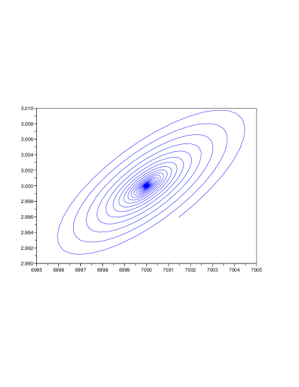
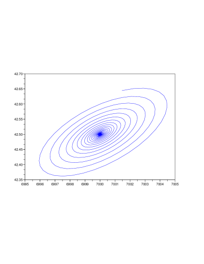
The direct analysis of this computer model confirms Theorem 3.2. We test the behavior of all coordinates to step. We observe, they demonstrate the following features. Each coordinate of all three vectors goes to an appropriate value when . In the phase spaces we get the perfect spirals which twist to the equilibrium point: with the arithmetic mean values of the initial dates.
It is important, that in the phase spaces and we get different spirals which twist in the opposite directions to points and respectively. We remark that values and oscillate for a long time. They simultaneously approach under to the fixed means and which exactly are the middle values by regions of the starting distributions of the proper substances (see Fig. 1 – 2).
Considering of numerous examples, in particular, varying the values of the initial coordinates demonstrate the stable character of the equilibrium state. No doubt, the state of the conflict triad defined by the middle-arithmetic values is attractive for all trajectories close to this state. Thus, the proper point is a local attractor. Moreover, even large enough change of coordinates for the vector of biological populations (for example, the replacement by ) does not destroy the attracting property to the equilibrium state.
3.3 Cyclic attractors
The equilibrium state from the previous example (the locally stable fixed point) is not a global attractor. In particular, this state is vanished under the large enough change of single coordinate of the vector that corresponds to an epidemic infection. Of course, under any small variations of coordinates, the system does not leave the attracting phase to the equilibrium state. Nevertheless, the replacement by transforms our system into another behavior phase. We observed, in particular, the phase of attraction to the cyclic orbit. Under the change mentioned above all coordinates are not attracted to a fixed point (the equilibrium state) but approximate a cyclic trajectory. For more details, let us analyze the following example.
Example 2. The loss of the equilibrium state (a stable fixed point) may take place under some changing of the initial coordinates and even only one of them.
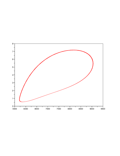
In particular, even changing of the initial values of any substances. So, replacing by we obtain the appearance of the cyclic attractor in the phase spaces and (see Fig. 3). That is, they are achieved quickly enough, already at step. It is interesting that cyclic oscillations of and take place around points which are shifted with respect to the arithmetic mean values of the initial coordinates (see the previous example).
How to explain this shift? There are also additional questions. For example, why a decrease of full mass of vital resource (from 170 to 130) leads also to passing of the system into the new phase? It is not attracted already by the fixed point. The evolution trajectory of the conflict triad approximates the cyclic orbit. They are attracted rather quickly to a cycle of the egg-like form. That is, in the limit all trajectories oscillate around fixed points which are shifted in comparison with the initial mean values. All these questions are open problems, although in [2] we made attempts to give some interpretations to the phenomena mentioned above.
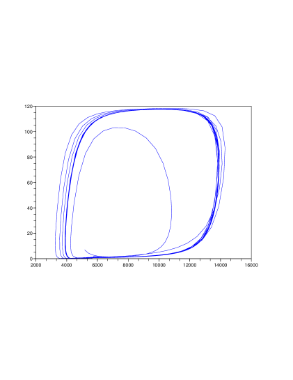
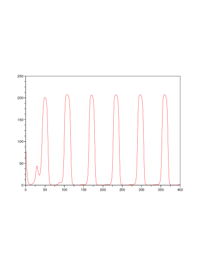
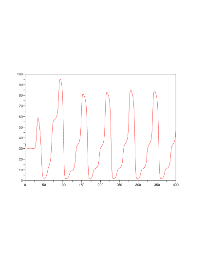
Example 3. The exponential increasing of the initial coordinates causes the appearance of almost square attractor in the phase space. That is, oscillates from zero to the maximal value, nearly 120. In particular, the replacement by induced the oscillations of large amplitude, up to 200! (See Fig. 4). In the same time the coordinates of resource vector have periodic oscillations without achievement of the absolute maximum.
These observations confirm an interesting practical effect. The substance which corresponds to negative threats (an epidemic infection) has large influence to the behavior of biological population. So, the relatively small increase of initial values of coordinates substantially multiplies the negative effect on other substances. Thus, the increasing of threats presses not only to the existence of biological population, but also at the resource environment. In particular, it makes impossible the achievement of maximal values by them (See Fig. 5,6).
3.4 The wave of cyclic attractors
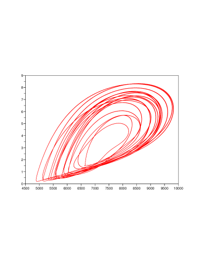
This phenomenon arises up under a certain increasing of parameters . We represent it at Fig. 7 where few cycles are observed and they imposed one at another. These cycles have different periods. In this case the trajectories are approximated consecutively to one of cyclic attractors, but only for some time. We call this picture the wave of cyclic attractors. Note that similar behavior of complex biological dynamical systems appear in practical situations, for example, in a case with several epidemic sources.
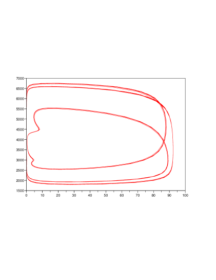
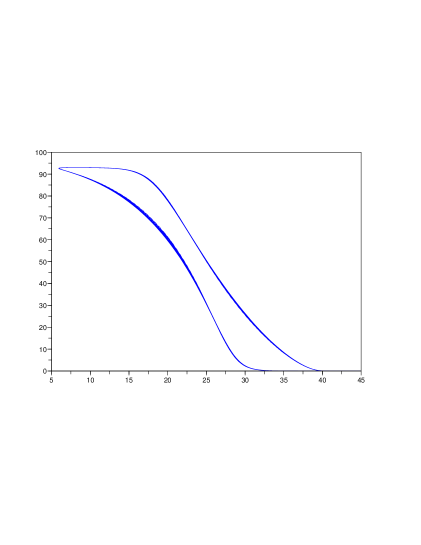
The cyclic attractors for orbits can have not only egg-like shape, but also considerably more difficult geometrical structures (see Fig. 8). In particular, the cyclic attractor similar to the -cycle (see Fig. 9) describes the behavior of a pair ”virus-resource”. It has close analogy with work of a move aggregate that consumes a certain resource, but survives resistance and have to come back at the starting position.
3.5 The quasi-chaotic behavior
At the computer model that corresponds to Fig. 8 we observe an obvious evolution non-balanced for biological population and infection, we call this dynamical phase as the quasi-chaotic behavior. Thus, any regularity is absent here and one can not find even a slightly noticeable low in the behavior. We may find some analogy with a chronic hidden disease, that is healed, but not cured. It increases non-periodically but does not reach a critical stage in an organism which passed some threshold in its development. In this situation it is impossible to go back to the state of attracting to a stable point of equilibrium without external influencing (See Fig. 9).
More deep analysis shows the presence of bifurcation points in some zones of phase space. Depending on parameter meanings and and initial values of coordinates, the evolution of the whole system passing this point may sharply change its direction. In particular, it is not structurally stable and can already not reach the equilibrium state.
4 Discussion
The main result of our work consists in the construction of complex models which demonstrate the presence of all basic phases for coexistence of typical conflict triad substances: the state of dynamical equilibrium (a stable fixed point), the phase of the limit cyclic attractors (trajectories with periodically pulsating evolution for each of substances), the area of bifurcation points, that corresponds, in particular, to series of the extremely complex behaviors with transitions between some cascade of cyclic attractors, and finally, the phase close to chaotic which we call the quasi-chaotic behavior. All these phases for coexistence of conflict substances one can meet rather often in reality. So, the state of dynamical equilibrium is typical for the simultaneous coexistence of different kinds of bacteria inside a living creature, when the highly dangerous microbes exist in a healthy organism but do not exceed a critical concentration and cause obvious rejections (that is an ordinary dynamical equilibrium). Although the considerable enough external impact is able to violate such equilibrium state and to result in creation of priorities to some kind of bacteria and symptoms of a certain illness. Other typical phase, the cyclic attractors, observed, for example, when the season (cyclic) flu epidemics are caused by exhausting of the valuable vital resources and by a too much concentration (an overpopulation) of biological species in some regions. This phase is character of most oscillating processes in our reality.
Certainly, the phases and states of the dynamical systems of conflict triad mentioned above appear only under appropriated values of parameters and starting coordinates. In the majority of situations we observe an extremely complex, sometimes practically chaotic behavior of our system. This all means that the theory developed here is in fact only an introduction to study of the conflict triad by the regional approach method. Of course, it can be applied as a research instrument for concrete tasks in conflicts with triple opponents.
It is important that our model in concrete settings allows to determine the probability of infection for considered biological species by an epidemic disease in each separate region of common space of existence. We recall that a key point of our constructions is a natural division of the whole territory of existence onto a set of regions with studying of the local process of conflict interactions. Thus, the complete picture of dynamical changes takes into account redistribution and migration processes between regions, both for biological species and for infections. In essence, a model gives not only the statistical picture of distributions but also the quantitative characteristics for each of interacting substances in regions at discrete time. It is possible to provide the prediction and information about the power of infection risk, periods of relative safety and picks of sharp growth of the infection density (epidemic) using the model. Besides, it is also possible to pick regions with relative stability or opposite ones with biggest growth of disease.
Finally we remark that it is possible to watch for sizes of relations such as which make sense of distribution densities of positive vital resources and threats of infection for existence of biological species in region. These sizes are important at the decision making problem for safe of existence of biological species in a fixed region. The error of uncertainty of such decisions depends on the range of changes for parameters which are controlled by external factors with respect to the system.
We hope that the dynamical model of conflict interaction between triple intrinsic elements offered here may be used as a flexible tool in the problem of practical forecasts. Among important dynamical parameters one can take such ones: the speed of reproduction and spread of infection, their density and the local concentration, the rates of migration between regions and so on.
References
- [1] A. Agliari, G.I. Bischi, L. Gardini, Some methods for the global analysis of dinamic games represented by noninvertible maps, In T.Puu I.Sushko (Edts.), Oligopoly Dynamics: Models and Tools, New York, Springer Verlag, 31-83 (2002).
- [2] S. Albeverio, V. Koshmanenko, I. Samoilenko, The conflict interaction between two complex systems: Cyclic migration, J. Interdisciplinary Math., 11 , No 2, 163-185, (2008).
- [3] S. Albeverio, M. Bodnarchyk, V. Koshmanenko, Dynamics of Discrete Conflict Interactions Between Non-annihilating Opponents, Methods Funtional Analasis and Topology, 11, no. 4, 309-319, (2005).
- [4] G.I. Bischi, M. Gallegati, L. Gardini, R. Leombruni, A. Palestrini, Herd behavior and nonfundamental asset price fluctuations in financial markets, Macroeconomic Dynamics, 10, 502-528 (2006).
- [5] G.I. Bischi, F. Tramontana, Three-dimansional discrete-time Lotka-Volterra models with an application to industrial clusters, Commun Nonlinear Sci Numer Simulat, 15, 3000–3014 (2010).
- [6] M.Bandyopadhyay, J.Chattopadhayay, Ratio-dependent predator-prey model: effects of environmental fluctuation and stability, Nonlinearity, No. 18, 913–936, (2005).
- [7] M. Bodnarchyk, V. Koshmanenko, . Samoilenko, Dynamics of the conflict intertaction between systems with internal structures, Nonlinear osccilation, 9, 4, 435-450, (2006).
- [8] J.M. Epstein, Nonlinear dynamics, mathematical biology, and social science, Addison-Wisley Publ.Com., 1997.
- [9] A. J. Jones, Game theory: mathematical models of conflict, Mathematics and its Applications. New York-Chichester-Brisbane, 1980.
- [10] J. Hofbauer, K. Sigmund, The Theory of Evolution and Dynamical Systems, Cambridge Univ. Press, 1988.
- [11] J. Hofbauer, K. Sigmund, Evolutionary Games and Population Dynamics, Cambridge Univ. Press, 1998.
- [12] V. Koshmanenko, On the Conflict Theorem for a Pair of Stochastic Vectors, Ukrainian Math. J., 55, No. 4, P. 555-560, (2003).
- [13] V. Koshmanenko, The Theorem of Conflict for Probability Measures, Math. Methods of Operations Research 59, No.2 (2004) 303–313.
- [14] V.D. Koshmanenko, N.V. Kharchenko, Invariant points of dynamical conflict system in the space of piecewise uniformly distributed measures, Ukrainian Math. J., 56, N 7, (2004) 927–938.
- [15] M.V. Bodnarchyk, V.D. Koshmanenko, N.V. Kharchenko, Properties of the limiting states of dynamical conflict system, Nonlinear oscillations, 7, N 4, (2004) 446-461.
- [16] V. Koshmanenko, N.Kharchenko, Spectral properties of image measures after conflict interactions, Theory of Stochastic Processes, 10(26), N 3-4, 73-81, (2004).
- [17] V.Koshmanenko, I.Samoilenko, The Conflict Dynamics of Natural Triad, Intern. Conference ”Problems of decision making under uncertainties” , PDMU-2008, Kyiv-Rivne, Ukraine, 25-26, (2008).
- [18] Y.Kuang, Basic properties of mathematical population models, J. Biomath, No. 17, 129–142, (2002).
- [19] Y.Kuang, E.Beretta, Global qualitative analysis of a ratio-dependent predator-prey system, J. Math. Biol., , No. 36, 389–406, (1998).
- [20] Y.Lonzonn, S.Solomon, J.Goldenberg, D.Mazarsky, World-size global markets lead to economic instability, Acrificial life, 357–370, (2003).
- [21] M.Maron, Modelling Populations: From Malthus to the Threshold of Artificial Life, Evolutionary and Adaptive Systems, Uni. of Sussex, 1-17, (2003).
- [22] J.D. Murray, Mathematical biology I: An Introduction, Springer, (2002).
- [23] J.D. Murray, Mathematical biology II: Spatial Models and Biomedical Apllications, Thried eddition, Springer, (2003).
- [24] G. Owen, Game theory, Third edition. Academic Press, Inc., San Diego, CA, 1995.
- [25] E.Renshaw, Modelling Biological Populations in Space and Time. Cambridge Uni. Press, 1991.
- [26] K.I.Takahashi, K.MD.M.Salam, Mathematical model of conflict with non-annihilating multi-opponent, J. Interdisciplinary Math., 9, No. 3, 459-473, (2006).