Insulating behavior in metallic bilayer graphene: Interplay between density inhomogeneity and temperature

Abstract

We investigate bilayer graphene transport in the presence of electron-hole puddles induced by long-range charged impurities in the environment. We explain the insulating behavior observed in the temperature dependent conductivity of low mobility bilayer graphene using an analytic statistical theory taking into account the non-mean-field nature of transport in the highly inhomogeneous density and potential landscape. We find that the puddles can induce, even far from the charge neutrality point, a coexisting metallic and insulating transport behavior due to the random local activation gap in the system.

Recent experiments Zhu et al. (2009); Feldman et al. (2009); Fuhrer ; Zhu ; herrero2010 ; ki2010 have revealed an intriguingly strong (and anomalous) “insulating” temperature dependence in the measured electrical conductivity of bilayer graphene (BLG) samples, not only at the charge neutrality point (CNP) where the electron-hole bands touch each other (with vanishing average carrier density), but also at carrier densities as high as $10^{12}$ cm^-2 or higher. (“Insulating” temperature dependence of conductivity $\sigma(T)$ simply means an increasing $\sigma$ with increasing temperature at a fixed gate voltage, which is, in general, considered unusual in a nominally metallic system where the resistivity, not the conductivity, should increase with temperature.) Such an anomalous insulating temperature dependence of $\sigma(T)$ is typically not observed in monolayer graphene (MLG) away from the CNP although the gate voltage (or equivalently, the density) dependence of MLG and BLG conductivities are very similar with both manifesting linear-in-density conductivity away from the CNP and an approximately a constant minimum conductivity around the CNP Morozov et al. (2008); Xiao et al. (2009).

In this Letter we theoretically establish that this anomalous insulating BLG $\sigma(T)$ behavior is likely to be caused by the much stronger BLG density inhomogeneity Das Sarma et al. (2010) (compared with MLG) which gives rise to a qualitatively new type of temperature dependence in graphene transport, namely, the intriguing coexistence of both metallic and activated transport, hitherto not discussed in the literature. We therefore predict that the observed temperature dependence of BLG $\sigma(T)$ arises from the same charged impurity induced puddles in the system which are responsible for the minimum conductivity plateau at the CNP Das Sarma and Shaffique Adam (2010). We provide an analytic theory which appears to be in excellent qualitative agreement with the existing experimental results. One direct prediction of our theory, the suppression of the anomalous insulating temperature dependence in high mobility samples with lower disorder, seems to be consistent with experimental observations. As a direct corollary of our theory, we find, consistent with experimental observation Castro et al. (2007); Oostinga and Hubert B. Heersche (2008); Mak et al. (2009), that a gapped BLG (with the gap at the CNP induced, for example, by an external electric field) would typically manifest a transport activation gap substantially smaller than the intrinsic spectral gap (i.e. the energy band gap) unless the band gap is much larger than the typical puddle-induced potential energy fluctuations.

Our theory is based on a physically motivated idea: In the presence of large potential fluctuations $V({\bf r})$, the local Fermi level, $\mu({\bf r})=E_{F}-V({\bf r})$, would necessarily have large spatial fluctuations [particularly when $E_{F}\lesssim s$, where $s=V_{rms}$ is the root-mean-square fluctuations or the standard deviation in $V({\bf r})$], leading to a complex temperature dependence of transport since both metallic and activated transport would be present due to random local gap. Below we carry out an analytical theory implementing this physical idea. We will see that this physical idea leads to the possible coexistence of metallic and activated transport, which explains the observed temperature dependence of BLG transport.

We start by assuming that the disorder-induced potential energy fluctuations in the BLG is described by a distribution function $P(V)$ which $V=V({\bf r})$ is the fluctuating potential energy at the point ${\bf r}\equiv(x,y)$ in the 2D BLG plane. We approximate the probability $P(V)dV$ of finding the local electronic potential energy within a range $dV$ about $V$ to be a Gaussian form, i.e., $P(V)=\frac{1}{\sqrt{2\pi s^{2}}}\exp(-V^{2}/2s^{2})$, where $s$ is the standard deviation (or equivalently, the strength of the potential fluctuation). Then in the presence of electron-hole puddles the density of states (DOS) is reduced by the allowed electron region fraction and given by $D(E)=\int_{-\infty}^{E}D_{0}P(V)dV={D_{0}}{\rm erfc}(-E/\sqrt{2}s)/2$, where erfc$(x)$ is the complementary error function and $D_{0}={g_{s}g_{v}m}/(2\pi\hbar^{2})$ is the DOS in a homogeneous system, where $m$ is the band effective mass, $g_{s}=2$ and $g_{v}=2$ are the spin and valley degeneracies, respectively. We have $D_{0}=2.8\times 10^{10}$ cm^-2/meV with the effective mass $m=0.033m_{e}$ (where $m_{e}$ is the bare electron mass). Note that the tail of the DOS is determined by the potential fluctuation strength $s$.

Since BLG is a gapless semiconductor the electron density at finite temperature increases due to the direct thermal excitation from valence band to conduction band, and this thermal excitation is an important source of temperature dependent transport. Thus, we first consider the temperature dependence of thermally excited electron density. The total electron density is given by

$$n_{e}=\int_{-\infty}^{\infty}D(E)\frac{dE}{e^{\beta(E-E_{F})}+1},$$ (1)

where $\beta=1/k_{B}T$ and $E_{F}$ is the Fermi energy. When the Fermi energy is zero (or at CNP) all electrons are located in the band tail at $T=0$ and the electron density in the band tail is given by $n_{0}=n_{e}(E_{F}=0)={D_{0}s}/{\sqrt{2\pi}}$. Note that the electron density in the band tail is linearly proportional to the standard deviation $s$. At finite temperatures we find the asymptotic behavior of $n_{0}(T)$. The low temperature ($k_{B}T/s\ll 1$) behavior of electron density at CNP becomes

$$n_{e}(T)=n_{0}\left[1+\frac{\pi^{2}}{6}\left(\frac{k_{B}T}{s}\right)^{2}\right].$$ (2)

Thus, the electron density increases quadratically in low temperature limit. For homogeneous BLG with the constant DOS the electron density at finite temperatures is given by $n_{e}(T)=D_{0}\ln(2)k_{B}T$. The presence of the band tail suppresses the thermal excitation of electrons and gives rise to the quadratic behavior. However, at high temperature the density increases linearly with the same slope as in the homogeneous system, i.e.,

$$n(T)\sim D_{0}\left[\ln(2)k_{B}T+\frac{1}{8}\frac{s^{2}}{(k_{B}T)^{2}}\right].$$ (3)

In Fig. 1(a) we show the temperature dependent electron density at CNP for different standard deviations.

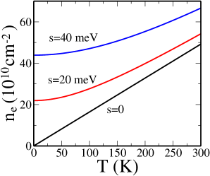
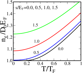
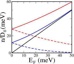
Figure 1: (Color online) (a) The electron density at CNP as a function of temperature for different $s$. At $T=0$ the density is given by $n_{0}=D_{0}s/\sqrt{2\pi}$. (b) The temperature dependent electron density at finite $E_{F}$ for different $s$. For $s/E_{F}\neq 0$ the leading order behavior is quadratic while at $s=0$ the density is exponentially suppressed. (c) Total electron densities (solid lines) and hole densities (dashed lines) as a function of $E_{F}$ for two different $s=30$ meV and 70 meV. The linear line represents the density difference $n=n_{e}-n_{h}=D_{0}E_{F}$, which linearly depends on the Fermi energy. The densities at the band tails are given by $n_{e}(E_{F}=0)=n_{h}(E_{F}=0)=D_{0}s/\sqrt{2\pi}$.

In the case of finite doping (or gate voltage), i.e., the Fermi level away from CNP, $E_{F}\neq 0$, the electron density of the homogeneous BLG for $s=0$ is given by

$$n_{0e}(T)=D_{0}E_{F}\left[1+t\ln\left(1+e^{-1/t}\right)\right],$$ (4)

where $t=T/T_{F}$ and $T_{F}=E_{F}/k_{B}$. At low temperatures ($T\ll T_{F}$) the thermal excitation is exponentially suppressed due to the Fermi function, but at high temperatures ($T\gg T_{F}$) it increases linearly. In the presence of electron-hole puddles ($s\neq 0$) we have the electron density at zero temperature for the inhomogeneous system:

$$n_{e}(0)={D_{0}E_{F}}\left[\frac{1}{2}{\rm erfc}\left(\frac{-1}{\sqrt{2}\tilde{s}}\right)+\frac{\tilde{s}}{\sqrt{2\pi}}e^{-1/2\tilde{s}^{2}}\right],$$ (5)

where $\tilde{s}=s/E_{F}$. At low temperatures ($T\ll T_{F}$) the asymptotic behavior of the electron density is given by

$$n_{e}(T)=n_{e}(0)+D_{0}E_{F}\frac{\pi^{2}}{12\sqrt{2}}\frac{e^{-1/2\tilde{s}^{2}}}{\tilde{s}}\left(\frac{T}{T_{F}}\right)^{2}.$$ (6)

The leading order term is the same quadratic behavior as in undoped BLG ($E_{F}=0$), but the coefficient is strongly suppressed by fluctuation. In the case of $s>E_{F}$, the existence of electron-hole puddles gives rise to a notable quadratic behavior [see Fig. 1(b)]. At high temperatures ($T\gg T_{F}$) we find

$$n_{e}(T)=n_{0e}(T)+\frac{D_{0}E_{F}}{(1+e^{\beta E_{F}})^{2}}\frac{\tilde{s}^{2}}{2}\frac{T_{F}}{T}.$$ (7)

At CNP ($E_{F}=0$) electrons and holes are equally occupied. As the Fermi energy increases, more electrons occupy increasingly larger proportion of space [see Fig. 1(c)]. For $E_{F}\gg s$ nearly all space is allowed to the electrons, and the conductivity of the system approaches the characteristic of the homogeneous materials. In the presence of electron-hole puddles, there is a possible coexistence of metallic and thermally-activated transport. When electron puddles occupy more space than hole puddles, most electrons follow the continuous metallic paths extended throughout the system, but it is possible at finite temperature that the thermally activated transport of electrons persists above the hole puddles. On the other hand, holes in hole puddles propagate freely, but when they meet electron puddles activated holes conduct over the electron puddles. Carrier transport in each puddle is characterized by propagation of weak scattering transport theory Das Sarma et al. (2010). The activated carrier transport of prohibited regions, where the local potential energy is $V$ less (greater) than Fermi energy for electrons (holes), is proportional to the Fermi factor. If $\sigma_{e}$ and $\sigma_{h}$ are the average conductivity of electron and hole puddles, respectively, then the activated conductivities are given by

$$\sigma_{e}^{(a)}(V) = \sigma_{e}\exp[\beta(E_{F}-V)],$$ (8a)

$$\sigma_{h}^{(a)}(V) = \sigma_{h}\exp[\beta(V-E_{F})],$$ (8b)

where the density and temperature dependent average conductivities ($\sigma_{e}$ and $\sigma_{h}$) are given within the Boltzmann transport theory Das Sarma et al. (2010) by $\sigma_{e}={n_{e}e^{2}\langle\tau\rangle}/{m}$ and $\sigma_{h}={n_{h}e^{2}\langle\tau\rangle}/{m}$, where $n_{e}$ and $n_{h}$ are average electron and hole densities, respectively, and $\langle\tau\rangle$ is the transport relaxation time which depends explicitly on the scattering mechanism Das Sarma et al. (2010).

Now we denote the electron (hole) puddle as region ‘1’ (‘2’). In region 1 electrons are occupied more space than holes when $E_{F}>0$. The fraction of the total area occupied by electrons with Fermi energy $E_{F}$ is given by $p=\int_{-\infty}^{E_{F}}P(V)dV$. Then the total conductivity of region 1 can be calculated

$$\sigma_{1} = \frac{1}{p}\int^{E_{F}}_{-\infty}(\sigma_{e}+\sigma_{h}^{(a)})P(V)dV,$$ (9)

$$= \sigma_{e}+\frac{\sigma_{h}}{2p}e^{\frac{\beta^{2}s^{2}}{2}-\beta E_{F}}{\rm erfc}\left(-\frac{E_{F}}{\sqrt{2}s}+\frac{\beta s}{\sqrt{2}}\right).$$

At the same time the holes occupy the area with a fraction $q=1-p$ and the total conductivity of region 2 becomes

$$\sigma_{2} = \frac{1}{q}\int_{E_{F}}^{\infty}(\sigma_{e}^{(a)}+\sigma_{h})P(V)dV$$ (10)

$$= \sigma_{h}+\frac{\sigma_{e}}{2q}e^{\frac{\beta^{2}s^{2}}{2}+\beta E_{F}}{\rm erfc}\left(\frac{E_{F}}{\sqrt{2}s}+\frac{\beta s}{\sqrt{2}}\right).$$

The $\sigma_{1}$ and $\sigma_{2}$ are distributed according to the binary distribution. The conductivity of binary system can be calculated by using the effective medium theory of conductance in mixturesKirkpatrick (1973). The result for a 2D binary mixture of components with conductivity $\sigma_{1}$ and $\sigma_{2}$ is given by Kirkpatrick (1973)

$$\sigma_{t}=(p-\frac{1}{2})\left[(\sigma_{1}-\sigma_{2})+\sqrt{(\sigma_{1}-\sigma_{2})^{2}+\frac{4\sigma_{1}\sigma_{2}}{(2p-1)^{2}}}\right].$$ (11)

This result can be applied for all Fermi energy. For a large doping case, in which the hole puddles disappear, we have $p=1$ and $\sigma_{2}=0$, then Eq. (11) becomes $\sigma=\sigma_{1}$, i.e., the conductivity of electrons in the homogeneous system.

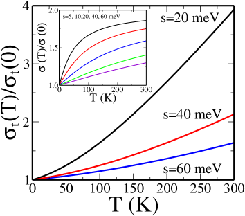
Figure 2: (Color online) $\sigma_{t}(T)$ at charge neutral point for different $s$. Inset shows the thermally activated conductivity as a function temperature.

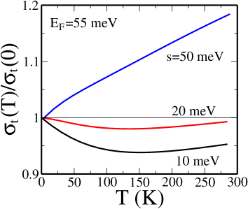
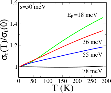
Figure 3: (Color online). (a) $\sigma_{t}(T)$ for $E_{F}=55$ meV and for different $s$. (b) $\sigma_{t}(T)$ for $s=50$ meV and for several $E_{F}=18$, 36, 55, 78 meV, which correspond to the densities $n=0.5,$ 1.0, 1.5, 2.0$\times 10^{12}$ cm^-2.

We first consider the conductivity at CNP ($E_{F}=0$). The conductivities in each region are given by

$$\sigma_{1} = \sigma_{e}\left[1+\frac{\eta}{2p}e^{\beta^{2}s^{2}/2}{\rm erfc}(\beta s/\sqrt{2})\right],$$ (12a)

$$\sigma_{2} = \sigma_{h}\left[1+\frac{1}{2q\eta}e^{\beta^{2}s^{2}/2}{\rm erfc}(\beta s/\sqrt{2})\right],$$ (12b)

where $\eta=n_{h}/n_{e}$ is the ratio of the hole density to the electron density. Since the electrons and holes are equally populated we have $p=q=1/2$ and $\sigma_{e}=\sigma_{h}$, then the total conductivity becomes $\sigma_{t}=\sqrt{\sigma_{1}\sigma_{2}}=\sigma_{1}$. The asymptotic behavior of the conductivity at low temperatures ($k_{B}T\ll s$) becomes

$$\sigma_{t}(T)=\sigma_{e}\left[1+\sqrt{\frac{2}{\pi}}\frac{k_{B}T}{s}-\frac{2}{\sqrt{\pi}}\frac{(k_{B}T)^{3}}{s^{3}}\right].$$ (13)

The activated conductivity increases linearly with a slope $\sqrt{2/\pi}k_{B}/s$ as temperature increases. Because $s$ is typically smaller in higher mobility sample, the high mobility samples show stronger insulating behavior at low temperatures. The next order temperature correction to conductivity arises from the thermal excitation given in Eq. (2) which gives $T^{2}$ corrections. Thus in low temperature limit the total conductivity at CNP is given by

$$\sigma_{t}(T)=\sigma(0)\left[1+\sqrt{\frac{2}{\pi}}\frac{k_{B}T}{s}+\frac{\pi^{2}}{6}\left(\frac{k_{B}T}{s}\right)^{2}\right].$$ (14)

At high temperatures ($k_{B}T\gg s$) we have

$$\sigma_{t}=\sigma_{e}\left[2-\sqrt{\frac{2}{\pi}}\frac{s}{k_{B}T}+\frac{s^{2}}{2(k_{B}T)^{2}}\right].$$ (15)

The total conductivity due to the activation behavior approaches a limiting value and all temperature dependence comes from the thermal excitation through the change of carrier density given in Eq. (3). Thus at very high temperatures ($T\gg s/k_{B}$) the BLG conductivity at the charge neutral point increases linearly with a universal slope $\ln(2)$ regardless of the sample quality. In Fig. 2 we show the calcuated temperature dependent conductivity at charge neutral point.

At finite doping ($E_{F}>0$) the temperature dependent conductivities are very complex because three energies ($E_{F}$, $s$, and $k_{B}T$) are competing. Especially when $k_{B}T\ll s$, regardless of $E_{F}$, we have the asymptotic behavior of conductivities in region 1 and 2 from Eqs. (9) and (10), respectively,

$$\sigma_{1} = \sigma_{e}\left[1+\frac{\eta}{2p}e^{-1/2\tilde{s}^{2}}\sqrt{\frac{2}{\pi}}\frac{1}{\tilde{s}/t-1/\tilde{s}}\right],$$ (16a)

$$\sigma_{2} = \sigma_{h}\left[1+\frac{1}{2q\eta}e^{-1/2\tilde{s}^{2}}\sqrt{\frac{2}{\pi}}\frac{1}{\tilde{s}/t+1/\tilde{s}}\right],$$ (16b)

where $\tilde{s}=s/E_{F}$ and $t=T/T_{F}$. The leading order correction is linear but the coefficient is exponentially suppressed by the term $\exp(-E_{F}^{2}/2s^{2})$. This fact indicates that in the high mobility sample with small $s$, the activated conductivity is weakly temperature dependent except around CNP, i.e. $E_{F}<s$. Since the density increase by thermal excitation is also suppressed exponentially by the same factor [see Eq. (6)] the dominant temperature dependent conductivity arises from the scattering time Das Sarma et al. (2010). On the other hand, for a low mobility sample with a large $s$, the linear temperature dependence due to thermal activation can be observed even at high densities $E_{F}\gtrsim s$.

In Fig. 3 we show the total conductivities (a) for a fixed $E_{F}$ and several $s$ and (b) for a fixed $s$ and several $E_{F}$. In total conductivity the activated insulating behavior competes with the metallic behavior due to the temperature dependent screening effect. When $s$ is small the activated behavior is suppressed. As a result the total conductivity manifests the metallic behavior Das Sarma et al. (2010). However, for large $s$ the activated temperature dependence behavior overwhelms the metallic temperature dependence, and the system shows insulating behavior.

Finally, we discuss three important issues: (1) The same physics, of course, also applies to MLG graphene, but the quantitative effects of inhomogeneity (i.e. the puddles) are much weaker since simple estimates show that the dimensionless potential fluctuation strength $\tilde{s}$ ($\equiv s/E_{F}$) is much weaker in MLG than in BLG because of the linear (MLG) versus constant (BLG) DOS in the two systems. In particular, $\tilde{s}_{BLG}/\tilde{s}_{MLG}\sim 32\sqrt{\tilde{n}}$ where $\tilde{n}=n/10^{10}$, and therefore $\tilde{s}_{BLG}\gg\tilde{s}_{MLG}$ upto $n=10^{13}$ cm^-2. Direct calculations Das Sarma et al. (2010) show that the self-consistent values of $s$ tend to be much larger in BLG than in MLG for identical impurity disorder. In very low mobility MLG samples, where $s$ is very large, the insulating behavior of temperature dependent resistivity can be observed at high densities even in MLG samplesTan et al. (2007); Heo et. al. (2010). (2) We have neglected all quantum tunneling effects in our consideration because they are unimportant except at very low temperatures. In particular, Klein tunneling is strongly suppressed in strong disorder Rossi et al. (2010). (3) In the presence of a BLG gap ($\Delta_{g}$), the situation becomes extremely complicated since four distinct energy scales ($s$, $E_{F}$, $k_{B}T$, $\Delta_{g}$) compete, and any conceivable temperature dependence may arise depending on the relative values of these four energy scales. It is, however, obvious that any experimental measurement of the activation gap ($\Delta_{a}$) in such an inhomogeneous situation will produce $\Delta_{a}\ll\Delta_{g}$ unless $\Delta_{g}\gg s$. The system is now dominated by a random local gap arising from the competition among $s$, $\Delta_{g}$, and $E_{F}$, and no simple activation picture would apply. This is precisely the experimental observations Castro et al. (2007); Oostinga and Hubert B. Heersche (2008); Mak et al. (2009).

Work supported by ONR-MURI and NRI-NSF-SWAN.

References

- Zhu et al. (2009) W. Zhu et al., Phys. Rev. B 80, 235402 (2009).
- (2) M. Fuhrer, private communication.
- (3) J. Zhu, private communication.
- (4) P. Jarillo-Herrero, private communication.
- (5) D. G. Ki et al., unpublished (2010).
- Feldman et al. (2009) B. Feldman et al., Nature Physics 5, 889 (2009).
- Morozov et al. (2008) S. V. Morozov et al., Phys. Rev. Lett. 100, 016602 (2008).
- Xiao et al. (2009) S. Xiao et al., arXiv:0908.1329 (2009).
- Das Sarma et al. (2010) S. Das Sarma et al., Phys. Rev. B 81, 161407 (2010).
- Das Sarma and Shaffique Adam (2010) S. Das Sarma et al., arXiv:1003.4731 (2010).
- Castro et al. (2007) E. V. Castro et al., Phys. Rev. Lett. 99, 216802 (2007).
- Oostinga and Hubert B. Heersche (2008) J. B. Oostinga et al. Nature Materials 7, 151 (2008).
- Mak et al. (2009) K. F. Mak et al., Phys. Rev. Lett. 102, 256405 (2009).
- Kirkpatrick (1973) S. Kirkpatrick, Rev. Mod. Phys. 45, 574 (1973).
- Tan et al. (2007) Y. W. Tan et al., Eur. Phys. J. Special Topics 148, 15 (2007).
- Heo et. al. (2010) J. Heo et. al., unpublished (2010).
- Rossi et al. (2010) E. Rossi et al., Phys. Rev. B 81, 121408 (2010).