Kazhdan-Lusztig polynomials and drift configurations

Abstract.

The coefficients of the Kazhdan-Lusztig polynomials $P_{v,w}(q)$ are nonnegative integers that are upper semicontinuous on Bruhat order. Conjecturally, the same properties hold for $h$-polynomials $H_{v,w}(q)$ of local rings of Schubert varieties. This suggests a parallel between the two families of polynomials. We prove our conjectures for Grassmannians, and more generally, covexillary Schubert varieties in complete flag varieties, by deriving a combinatorial formula for $H_{v,w}(q)$. We introduce drift configurations to formulate a new and compatible combinatorial rule for $P_{v,w}(q)$. From our rules we deduce, for these cases, the coefficient-wise inequality $P_{v,w}(q)\preceq H_{v,w}(q)$.

1. Introduction

1.1. Overview

This paper studies two families of polynomials $\{P_{v,w}(q)\}$ and $\{H_{v,w}(q)\}$ defined for pairs of permutations $v,w$ in the symmetric group $S_{n}$ (or more generally, any Weyl group $W$). The former family consists of the celebrated Kazhdan-Lusztig polynomials, which were introduced in [KazLus79] to study representations of Hecke algebras. There it was conjectured that $P_{v,w}(q)\in{\mathbb{Z}}_{\geq 0}[q]$. This was later established [KazLus80] by interpreting $P_{v,w}(q)$ as the Poincaré polynomial for Goresky-MacPherson’s local intersection cohomology for the torus fixed point $e_{v}$ of the Schubert variety $X_{w}$ in the complete flag variety ${\rm Flags}({\mathbb{C}}^{n})$.

A key contribution to the theory is R. Irving’s theorem [Irv88] that the $P_{v,w}(q)$ are upper semicontinuous: if $v^{\prime}\leq v\leq w$ in Bruhat order, then $P_{v,w}(q)\preceq P_{v^{\prime},w}(q)$, where “$\preceq$” means that, for each $i$, the coefficient of $q^{i}$ in $P_{v,w}(q)$ is weakly smaller than the coefficient of $q^{i}$ in $P_{v^{\prime},w}(q)$. Thus, the Kazhdan-Lusztig polynomials are measures of the singularities of Schubert varieties whose coefficient growth tracks the worsening pathology of singularities as one moves along torus invariant ${\mathbb{P}}^{1}$’s towards the “most singular” point $e_{id}\in X_{w}$. In particular, $P_{v,w}(q)=1$ if and only if $e_{v}\in X_{w}$ is a (rationally) smooth point.

Conversely, the desire for insight into the combinatorics of Kazhdan-Lusztig polynomials naturally leads to the basic problem of understanding where and how the singularities of Schubert varieties worsen. In view of this converse problem, the growth of any semicontinuous singularity measure of Schubert varieties is of interest. One seeks concrete comparisons of different measures; see, e.g., [WooYon08] and the references therein.

Specifically, a well-studied semicontinuous measure is given by the Hilbert-Samuel multiplicity ${\rm mult}_{e_{v}}(X_{w})$. However, while this contains useful local data about $X_{w}$, even more is carried by the ${\mathbb{Z}}$-graded Hilbert series of ${\rm gr}_{\mathfrak{m}_{e_{v}}}{\mathcal{O}}_{e_{v},X_{w}}$, the associated graded ring of the local ring ${\mathcal{O}}_{e_{v},X_{w}}$,

$${\rm Hilb}({\rm gr}_{{\mathfrak{m}}_{e_{v}}}{\mathcal{O}}_{e_{v},X_{w}},q)=\frac{H_{v,w}(q)}{(1-q)^{\ell(w)}},$$

where $\ell(w)={\rm dim}(X_{w})$ is the Coxeter length of $w$. In particular, ${\rm mult}_{e_{v}}(X_{w})=H_{v,w}(1)$.

Conjecturally, each $h$-polynomial $H_{v,w}(q)$ is also in ${\mathbb{Z}}_{\geq 0}[q]$, and moreover is upper semicontinuous, just as is the case for Kazhdan-Lusztig polynomials. These conjectures suggest that the growth of the coefficients of the two families of polynomials is somehow correlated. In this paper, we offer an examination in the Grassmannian case, and more generally in the case of covexillary Schubert varieties inside ${\rm Flags}({\mathbb{C}}^{n})$. There the nonnegativity and semicontinuity conjectures are proved by deriving a new combinatorial rule for $H_{v,w}(q)$. In addition, by introducing drift configurations as a model for the Kazhdan-Lusztig polynomials in these settings (after [LasSch81] and [Las95]), we prove the inequality $P_{v,w}(q)\preceq H_{v,w}(q)$. This combinatorial discovery further indicates the link between the two families; no alternative explanation via algebraic or geometric methods seems available at present.

Summarizing, the main thesis of this paper is that there exists a parallel between $\{P_{v,w}(q)\}$ and $\{H_{v,w}(q)\}$. Our basis for this perspective comes from proofs of compatible and positive combinatorial rules for the two families of polynomials.

1.2. Statements of the main conjecture and theorems

Recapitulating, this paper formulates, and constructs supporting combinatorics for, the following conjecture:

Conjecture 1.1.

The $h$-polynomials $H_{v,w}(q)$ have nonnegative integral coefficients. In addition, they are upper semicontinuous, i.e., if $v^{\prime}\leq v$ in Bruhat order then $H_{v,w}(q)\preceq H_{v^{\prime},w}(q)$.

The nonnegativity claim would actually be immediate if ${\rm gr}_{{\mathfrak{m}}_{e_{v}}}{\mathcal{O}}_{e_{v},X_{w}}$ is Cohen-Macaulay (see Section 2.2). However, this latter assertion seems to be a folklore conjecture. Although ${\mathcal{O}}_{e_{v},X_{w}}$ is itself Cohen-Macaulay [Ram85], this property might be lost when degenerating to ${\rm gr}_{{\mathfrak{m}}_{e_{v}}}{\mathcal{O}}_{e_{v},X_{w}}$. On the other hand, the results detailed in this paper and in [LiYon10] also support the Cohen-Macaulayness conjecture. In particular, it would follow from the stronger claim [LiYon10, Conjecture 8.5] asserting the vertex decomposability of Stanley-Reisner simplicial complexes of certain Gröbner degenerations of Kazhdan-Lusztig varieties.

The semicontinuity claim is itself a strengthening of the nonnegativity claim since the smoothness of $X_{w}$ at $e_{w}$ implies $H_{w,w}(q)=1$. Furthermore, although the betti numbers of ${\rm gr}_{{\mathfrak{m}}_{e_{v}}}{\mathcal{O}}_{e_{v},X_{w}}$ are semicontinuous, the coefficients of $H_{v,w}(q)$ are an involved, signed expression in terms of those numbers. Therefore, this semicontinuity phenomenon seems substantive.

The natural projection map

$$\pi:{\rm Flags}({\mathbb{C}}^{n})\twoheadrightarrow{\rm Gr}_{k}({\mathbb{C}}^{n}):\ \ \ (\langle 0\rangle\subset F_{1}\subset\cdots\subset F_{k}\subset\cdots\subset F_{n-1}\subset{\mathbb{C}}^{n})\mapsto F_{k},$$

where ${\rm Gr}_{k}({\mathbb{C}}^{n})$ is the Grassmannian of $k$-dimensional planes in ${\mathbb{C}}^{n}$, is a fibration: local properties of torus fixed points $e_{\mu}\in X_{\lambda}\subseteq{\rm Gr}_{k}({\mathbb{C}}^{n})$ for Young diagrams $\lambda,\mu\subseteq k\times(n-k)$, are equivalent to local properties of $e_{v}\in X_{w}\subseteq{\rm Flags}({\mathbb{C}}^{n})$ where $v,w\in S_{n}$ are maximal Coxeter length representatives of $\lambda,\mu$ where the latter are thought of as cosets of $S_{n}/(S_{k}\times S_{n-k})$; see, e.g., [Bri03, Example 1.2.3]. These $v$ and $w$ are cograssmannian, i.e., they have a unique ascent, at position $k$: $v(k)<v(k+1)$ and $w(k)<w(k+1)$.

Lifting Grassmannian problems to ${\rm Flags}({\mathbb{C}}^{n})$ has the advantage of allowing one to embed them within the wider class of covexillary Schubert varieties $X_{w}$, i.e., where $w$ is $3412$-avoiding: there are no indices $i_{1}<i_{2}<i_{3}<i_{4}$ such that $w(i_{1}),w(i_{2}),w(i_{3}),w(i_{4})$ are in the same relative order as $3412$. This class appears more tractable than general flag Schubert varieties since it shares many of the same features as Grassmannian Schubert varieties. However, there is a salient difference: Grassmannian Schubert varieties are locally defined by equations that are homogeneous with respect to the standard grading that assigns each variable degree one. In general, this is not true in the covexillary case. This homogeneity means that taking associated graded of the local ring essentially does nothing, and so ${\rm gr}_{{\mathfrak{m}}_{e_{v}}}{\mathcal{O}}_{e_{v},X_{w}}$ is automatically Cohen-Macaulay; see, e.g., [LiYon10, Section 1] and Section 2.2.

The covexillary condition has already attracted significant attention; see, e.g., [LakSan90, Las95, Man01a, KnuMil05, KnuMilYon08, KnuMilYon09, LiYon10] and the references therein. In particular, [KnuMil05, Section 2.4] connects the condition to ladder determinantal ideals studied in commutative algebra. Our three main theorems below concern the covexillary setting, providing our main cases of support towards both our main thesis and Conjecture 1.1.

One of our results is to prove the following link between $H_{v,w}(q)$ and $P_{v,w}(q)$:

Theorem 1.2.

For $w$ covexillary, $P_{v,w}(q)\preceq H_{v,w}(q)$ and $\deg P_{v,w}(q)=\deg H_{v,w}(q)$.

While the Grassmannian case per se is new and supports our thesis, the covexillary generality also further highlights the amenability of covexillary Schubert varieties. Our proof of Theorem 1.2 is based on a new formula for covexillary Kazhdan-Lusztig polynomials. An earlier rule was given by A. Lascoux [Las95], generalizing his earlier Grassmannian rule with M.-P. Schützenberger [LasSch81] (for more recent treatments of the Grassmannian case see, e.g., [ShiZin10, JonWoo10]). Our formulation of a covexillary rule is in terms of drift configurations. It is entirely graphical and is perhaps more handy to compute.

To state our rule we use standard combinatorics of the symmetric group, see, e.g., [Man01a, Chapter 2] as well as some terminology introduced in [LiYon10] (the reader may wish to compare Examples 1.5 and 1.6 below with what follows). Let $w\in S_{n}$ be covexillary. Superimpose the graph $G(v)$ of $v$ drawn with dots $\circ$ in positions $(n-w(j)+1,j)$ on top of the diagram

$$D(w)=\{(i,j):i<n-w(j)+1,\textrm{ and }j<w^{-1}(n-i+1)\}\subset[n]\times[n].$$

Throughout, we use the convention that rows are indexed from bottom to top, and columns are indexed from left to right. Move each box ${\mathfrak{e}}$ of the essential set

$${\mathcal{E}}(w)=\{(i,j)\in D(w):(i+1,j),(i,j+1)\notin D(w)\}$$

diagonally southwest by the number of dots of $G(v)$ weakly southwest of ${\mathfrak{e}}$. Call the resulting boxes $\{{\mathfrak{e}}^{\prime}\}$, and define $B(v,w)$ to be the smallest Young diagram that contains $\{{\mathfrak{e}}^{\prime}\}$ and $(1,1)$ (we use French convention for our Young diagrams). The shape $\lambda(w)$ of $w$ is obtained by sorting the vector counting the number of boxes in nonempty rows of $D(w)$ into decreasing order. Now, draw $\lambda(w)$ in the southwest corner of $B(v,w)$.

Declare that any corner of $\lambda(w)$ is $0$-special. Let ${\rm arm}(b)$ (respectively, ${\rm leg}(b)$) refer to the boxes in $\lambda(w)$ strictly to the right (above) of $b$ and in the same row (column). Inductively, a box $b\in\lambda(w)$ is $z$-special, for $z\in{\mathbb{N}}$ if it is maximally northeast subject to

• $|{\rm leg}(b)|=|{\rm arm}(b)|$; and

• none of the boxes of $\{b\}\cup{\rm arm}(b)\cup{\rm leg}(b)$ are $y$-special for any $y<z$.

A box is ${\bf special}$ if it is $z$-special for some $z$. The continent of a special box $b$ is the set of $x\in\lambda(w)$ such that $b$ is the maximally northeast special box that is weakly southwest of $x$. The union of continents is ${\rm Pangaea}(v,w)\subseteq\lambda(w)$ (the set difference being an immovable reference continent).

Definition 1.3.

A drift configuration ${\mathcal{D}}$ is a non-overlapping configuration of continents inside $B(v,w)$, such that

• each special box is diagonally weakly northeast of its position in ${\rm Pangaea}(v,w)$; and

• relative southwest-northeast positions of special cells are maintained.

Let ${\rm drift}(v,w)$ be the set of all such ${\mathcal{D}}$ and let ${\rm wt}({\mathcal{D}})$ be the total distance traveled by the continents from ${\rm Pangaea}(v,w)$. Consider the generating series

$$Q_{v,w}(q)=\sum_{{\mathcal{D}}\in{\rm drift}(v,w)}q^{{\rm wt}({\mathcal{D}})}.$$

Theorem 1.4.

If $v,w\in S_{n}$ and $w$ is covexillary then:

• $P_{v,w}(q)=Q_{v,w}(q)$.

• If we instead take every box of $\lambda(w)$ to be a separate “country”, each of which “drifts” according to the rules of Definition 1.3, the total number of drift configurations is ${\rm mult}_{e_{v}}(X_{w})$; hence $P_{v,w}(1)\leq{\rm mult}_{e_{v}}(X_{w})$ is manifest from (I).

• There is a vertex decomposable (thus shellable) simplicial complex ${\rm KL}_{v,w}$ that is homeomorphic to a ball or a sphere, and whose facets are labeled by ${\mathcal{D}}\in{\rm drift}(v,w)$.

Our proof of (I) is a bijection with A. Lascoux’s rule (which descends to a bijection with the rule of [LasSch81] for Grassmannians). The multiplicity rule from (II) just restates the theorem from [LiYon10] (cf. the Grassmannian rule of [IkeNar09]). Although the inequality of (II) is a consequence of Theorem 1.2, we are emphasizing that our rule from (I) is compatible with our multiplicity rule and makes the inequality transparent. Actually, whether such an inequality might exist was first asked to us (independently) by S. Billey and A. Woo. Afterwards, H. Naruse informed us that he has a proof for all cominuscule $G/P$. These questions and results provided us initial motivation for our work towards Theorem 1.4. Note that as with the more general inequality of Theorem 1.2, this inequality is not true in general. For example, $P_{13425,34512}(1)=3$ while ${\rm mult}_{e_{13425}}(X_{34512})=2$.

The statement (III) is derived from [KnuMilYon08]. It points out a further resemblance to the combinatorics of ${\rm mult}_{e_{v}}(X_{w})$ in [LiYon10], where a similar complex also appears.

Example 1.5.

Figure 1 depicts ${\rm Pangaea}(v,w)$ with six (colored) continents where

$$w=\underline{20}\;\underline{19}\;\underline{18}\;\underline{11}\;\underline{10}\;9\;8\;\underline{12}\;\underline{17}\;\underline{16}\;7\;6\;\underline{15}\;\underline{14}\;\underline{13}\;5\;4\;3\;2\;1,\mbox{\ and $v=id$.\ \ \ \ \ \ \ \ \ \ \ \ \ \ \ \ \ \ \ \ \ \ \ \ \ \ \ \ \qed}$$

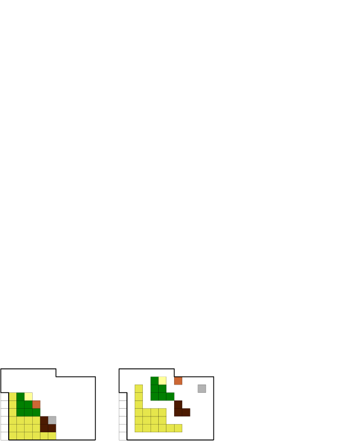
Figure 1. ${\rm Pangaea}(v,w)$ and a particular ${\mathcal{D}}\in{\rm drift}(v,w)$; ${\rm wt}({\mathcal{D}})=14$

Example 1.6.

Let $w=\underline{10}954382761$, $v=234651789\underline{10}$. Here $\lambda(w)=(4,4,3)$. Starting from $D(w)$, and the overlaid dots $\circ$ of $G(v)$, we derive $B(v,w)$. The special boxes are marked by $+$’s. See Figure 2.

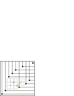
Figure 2. An overlay of $D(w)$ with $G(w)$ ($\bullet$’s) and $G(v)$ ($\circ$’s); constructing $B(v,w)$

Now ${\mathcal{E}}(w)=\{{\mathfrak{e}}_{1},{\mathfrak{e}}_{2}\}$ (being the maximally northeast boxes of each connected component of $D(w)$) move to $\{{\mathfrak{e}}_{1}^{\prime},{\mathfrak{e}}_{2}^{\prime}\}$, as determined by the $\circ$’s of $G(v)$. The five drift configurations are shown in Figure 3.

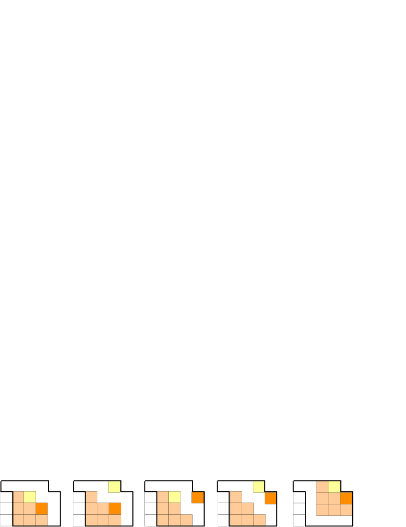
Figure 3. Drift configurations for $Q_{234651789\underline{10},\underline{10}954382761}(q)=1+2q+q^{2}+q^{3}$

∎

Our proof of Theorem 1.2 also depends on a new (and the first manifestly positive) combinatorial rule for covexillary $H_{v,w}(q)$. It additionally implies special cases of the nonnegativity and upper semicontinuity conjectures. Identify a partition $\lambda=(\lambda_{1}\geq\cdots\geq\lambda_{\ell}>0)$ with its Young diagram (in French notation). Recall, a Young tableau $T$ of shape $\lambda$ is semistandard if it is weakly increasing along rows and strictly increasing up columns. Given a vector $\textbf{b}=(b_{1},\dots,b_{\ell})$, we say $T$ is flagged by ${\bf b}$ if each entry in row $i$ is at most $b_{i}$. Let ${\rm SSYT}(\lambda,{\bf b})$ denote the set of semistandard Young tableaux flagged by ${\bf b}$. A (nonempty) set-valued filling is semistandard if each tableau obtained by choosing a singleton from each set gives a semistandard tableaux in the above sense [Buc00]. Similarly, we define flagged set-valued semistandard tableaux, and the set ${\rm SetSSYT}(\lambda,{\bf b})$ [KnuMilYon08].

Define $U\in{\rm SetSSYT}(\lambda,{\bf b})$ to be lower saturated if no smaller number can be added to any box $U(i,j)$ while maintaining semistandardness, i.e., in symbols, each

$$U(i,j)=[\alpha,\beta]:=\{\alpha,\alpha+1,\dots,\beta-1,\beta\},$$

for some $\alpha,\beta$ (depending on $i,j$) where

$$\alpha=\max\big{\{}\max U(i,j-1),1+\max U(i-1,j)\big{\}}.$$

Our convention for lower saturated tableaux is that $U(i,0)=1$ for all $i>0$ and $U(0,j)=0$ for all $j>0$. Let

$${\rm Lower}(\lambda,{\bf b})\subseteq{\rm SetSSYT}(\lambda,{\bf b})$$

denote this subset of lower saturated tableaux.

Define the saturation ${\rm sat}(T)\in{\rm Lower}(\lambda,{\bf b})$ of $T\in{\rm SSYT}(\lambda,{\bf b})$ to be

$${\rm sat}(T)(i,j)=[\max\{T(i,j-1),1+T(i-1,j)\},T(i,j)].$$

For $U\in{\rm SetSSYT}(\lambda,{\bf b})$, let

$${\rm ex}(U)=|U|-|\lambda|,$$

where $|U|$ refers to the number of entries of $U$ and $|\lambda|=\lambda_{1}+\lambda_{2}+\cdots$.

Finally, if $T\in{\rm SSYT}(\lambda,{\bf b})$ set

(1.1) $${\rm depth}(T):={\rm ex}({\rm sat}(T))=|{\rm sat}(T)|-|T|.$$

If $\lambda(w)=(\lambda(w)_{1}\geq\cdots\geq\lambda(w)_{\ell}>0)$ then define ${\bf b}={\bf b}(\Theta_{v,w})=(b_{1},\dots,b_{\ell})$ by

$$b_{i}=\max\{m:\;B(v,w)_{m}\geq\lambda(w)_{i}+m-i\}.$$

This is the maximum distance that the rightmost box in row $i$ can drift diagonally northeast within $B(v,w)$ (ignoring presence of other boxes).

Theorem 1.7.

Let $w\in S_{n}$ be covexillary. Then

$$H_{v,w}(q)=\sum_{T\in{\rm SSYT}(\lambda(w),{\bf b}(\Theta_{v,w}))}q^{{\rm depth}(T)}=\sum_{U\in{\rm Lower}(\lambda(w),{\bf b}(\Theta_{v,w}))}q^{{\rm ex}(U)}.$$

Moreover, Conjecture 1.1 is true under the hypothesis.

Example 1.8.

For $n=5$, $w=52341$, $v=12345$. There are five semistandard tableaux of shape $(2,1)$ and flagged by $(2,3)$:

$${2}$$

   

   

   

   

Their saturations are:

$${2}$$

   

   

   

   

The corresponding ${\rm ex}$ values are:

$$0,1,1,2,1.$$

Thus by Theorem 1.7, $H_{v,w}(q)=1+3q+q^{2}.$∎

Example 1.9.

Continuing Example 1.8, there are four drift configurations of the two continents,

The Kazhdan-Lusztig polynomial $P_{v,w}(q)=1+2q+q^{2}$. We see that $P_{v,w}(q)\preceq H_{v,w}(q)$, in agreement with Theorem 1.2.∎

1.3. Organization and contents

In Section 2, we state some preliminaries and further discuss Conjecture 1.1. We then prove Theorem 1.7. In Section 3, we briefly recall, for comparison, basics about Kazhdan-Lusztig theory. We then prove Theorem 1.2 while temporarily assuming Theorem 1.4(I). Section 4 is devoted to the construction of the simplicial complex of Theorem 1.4(II) and proof of its asserted properties. We furthermore define polynomials generalizing $Q_{v,w}(q)$ that naturally arise from this complex. In Section 5 we prove Theorem 1.4(I). We end that section with two comments (Remarks 5.5 and 5.6) about further properties of $P_{v,w}(q)$ that can be deduced from the rule. In Section 6, we give a formula for a different “$q$-analogue” of ${\rm mult}_{e_{v}}(X_{w})$ than $H_{v,w}(q)$. In Section 7, we offer some final remarks.

2. Hilbert series of the local ring ${\mathcal{O}}_{e_{v},X_{w}}$

2.1. Preliminaries

We use the usual identification ${\rm Flags}({\mathbb{C}}^{n})=GL_{n}/B$ where $B$ is the Borel subgroup consisting of invertible upper triangular matrices. Thus $GL_{n}$ acts on ${\rm Flags}({\mathbb{C}}^{n})$ by left multiplication, as does $B$, and the torus $T$ of invertible diagonal matrices. For each $v\in S_{n}$, let $e_{v}$ denote the associated $T$-fixed point. The Schubert cell $X_{w}^{\circ}:=Be_{w}$ while its Zariski closure is the Schubert variety $X_{w}={\overline{X_{w}^{\circ}}}$, an irreducible variety of dimension $\ell(w)$. We have that $e_{v}\in X_{w}$ if and only if $v\leq w$ in Bruhat order. A neighborhood of each point $p\in X_{w}$ is isomorphic to a neighborhood of some $e_{v}$, by the action of $B$. Hence, it suffices to restrict attention to $T$-fixed points. Let $B_{-}$ be the opposite Borel subgroup of invertible lower triangular matrices. If we set $\Omega_{v}^{\circ}=B_{-}vB/B$ to be the opposite Schubert cell, then up to crossing by affine space, a local neighbourhood of $e_{v}\in X_{w}$ is given by the Kazhdan-Lusztig variety ${\mathcal{N}}_{v,w}=X_{w}\cap\Omega_{v}^{\circ}$ [KazLus79, Lemma A.4].

Suppose $p$ is a point on a scheme $Y$. Let ${\rm gr}_{{\mathfrak{m}}_{p}}{\mathcal{O}}_{p,Y}$ denote the associated graded ring of the local ring ${\mathcal{O}}_{p,Y}$ with respect to its maximal ideal ${\mathfrak{m}}_{p}$, i.e.,

$${\rm gr}_{{\mathfrak{m}}_{p}}{\mathcal{O}}_{p,Y}=\bigoplus_{i\geq 0}m_{p}^{i}/m_{p}^{i+1}.$$

Since ${\rm gr}_{{\mathfrak{m}}_{p}}{\mathcal{O}}_{p,Y}$ picks up a ${\mathbb{Z}}$-grading, it now makes sense to discuss its Hilbert series. One can always express this series in the form

$${\rm Hilb}({\rm gr}_{{\mathfrak{m}}_{p}}{\mathcal{O}}_{p,Y},q)=\frac{H_{p,Y}(q)}{(1-q)^{\dim Y}}$$

where $H_{p,Y}(q)\in{\mathbb{Z}}[q]$ is the $h$-polynomial associated to $p\in Y$. It follows from standard facts that $H_{p,Y}(1)={\rm mult}_{p}(Y)$; see, e.g., [KreRob05, Theorem 5.4.15]. Hence $H_{p,Y}(q)=1$ if and only if $Y$ is smooth at $p$. In addition, note $H_{p,Y}(0)=1$, since this is the dimension of the zero graded piece of ${\rm gr}_{{\mathfrak{m}}_{p}}{\mathcal{O}}_{p,Y}$, i.e., the dimension of the field ${\mathcal{O}}_{p,Y}/{\mathfrak{m}}_{p}$.

Now, for any $v,w\in S_{n}$, we define $H_{v,w}(q)\in\mathbb{Z}[q]$ to be the $h$-polynomial associated to $e_{v}\in X_{w}$. At present, there is no purely combinatorial formula (even non-positive or recursive) for computing $H_{v,w}(q)$. However, instead one can utilize the explicit coordinates and equations for the ideal $I_{v,w}$ to define ${\mathcal{N}}_{v,w}={\rm Spec}\left({\mathbb{C}}[z^{(v)}]/I_{v,w}\right)$, as done in [WooYon08, Section 3.2]. Then one can Gröbner degenerate ${\mathcal{N}}_{v,w}$ to a scheme theoretic union of coordinate subspaces ${\mathcal{N}}_{v,w}^{\prime}$, using any of the term orders $\prec_{v,w,\pi}$ from [LiYon10, Section 3]. As explained in Theorem 3.1 (and its proof) of [LiYon10], the stated Gröbner degenerations degenerate not only ${\mathcal{N}}_{v,w}$ but also its projectivized tangent cone ${\rm Proj}({\rm gr}_{{\mathfrak{m}}_{e_{v}}}{\mathcal{O}}_{e_{v},X_{w}})$. Therefore the $h$-polynomial of ${\mathcal{N}}_{v,w}^{\prime}$ equals $H_{v,w}(q)$.

2.2. Conjectures

Let us now return to the discussion of Conjecture 1.1. Using the method for computing $H_{v,w}(q)$ summarized above, we obtained exhaustive checks for $n\leq 7$ of the following claim, restated from the introduction:

Nonnegativity conjecture.

$H_{v,w}(q)\in{\mathbb{Z}}_{\geq 0}[q]$.

In [LiYon10, Conjecture 8.5] we conjectured that within the family of term orders $\prec_{v,w,\pi}$, at least one gives a Gröbner limit scheme ${\mathcal{N}}_{v,w}^{\prime}$ that is reduced, equidimensional and whose Stanley-Reisner simplicial complex $\Delta_{v,w}$ is a vertex-decomposable ball or sphere. This implies in particular that $\Delta_{v,w}$ is shellable and thus Cohen-Macaulay. If this conjecture were true, it would follow that ${\rm gr}_{\mathfrak{m}_{e_{v}}}{\mathcal{O}}_{e_{v},X_{w}}$ is Cohen-Macaulay. Thus the nonnegativity Conjecture would hold by, e.g., [BruHer93, Corollary 4.1.10].

In the case that $I_{v,w}$ is a homogeneous ideal, with respect to the standard grading that assigns each variable degree $1$, since ${\mathcal{O}}_{e_{v},X_{w}}$ is Cohen-Macaulay [Ram85], it follows that the associated graded ring is Cohen-Macaulay; see e.g., [BruHer93, Exercise 2.1.27(c)]. Hence nonnegativity follows in this case. A. Knutson has shown that this homogeneity occurs whenever $w$ is $321$-avoiding [Knu09, pg. 25]. Moreover, in [WooYon09, Section 5] it was explained how “parabolic moving” reduces a large percentage of cases (for $n\leq 10$) to the homogeneous case. However, not every case can be so reduced, including those in the covexillary class. Thus, these cases provide further support for the above conjecture, separate from Theorem 1.7.

Upper semicontinuity conjecture.

If $v^{\prime}\leq v\leq w$ in Bruhat order, then $H_{v,w}(q)\preceq H_{v^{\prime},w}(q)$.

Unfortunately, even if we knew ${\rm gr}_{\mathfrak{m}_{e_{v}}}{\mathcal{O}}_{e_{v},X_{w}}$ to be Cohen-Macaulay, we do not know any way to express these coefficients in homological terms that would make the upper semicontinuity conjecture transparent. It should be noted that the proof of this property for Kazhdan-Lusztig polynomials in [Irv88] was not achieved using the geometry of Schubert varieties. However, see the geometric argument for the more general result [BraMac01, Theorem 3.6].

Although any proof of the above conjectures is desired, ideally one would also like combinatorial explanations of the properties.

Let us pause to collect some further facts for small $n$ in the following computational result. For (D) below we refer the reader to [WooYon08, Section 2.1] for the definition of interval pattern avoidance of $[x,y]\in S_{\infty}\times S_{\infty}$. There we explain that the existence of an interval pattern embedding guarantees ${\mathcal{N}}_{x,y}\cong{\mathcal{N}}_{\tilde{w},w}$, where $[x,y]\cong[\tilde{w},w]$ is an isomorphism of posets of Bruhat intervals in $S_{\infty}$. Thus, if the inequality $P_{x,y}(q)\preceq H_{x,y}(q)$ fails, so must $P_{\tilde{w},w}(q)\preceq H_{\tilde{w},w}(q)$.

Proposition 2.1.

• $\deg H_{v,w}(q)\leq\deg P_{v,w}(q)$ for $v\leq w\in S_{n}$ and $n\leq 6$.

• $\deg H_{v,w}(q)\leq\frac{\ell(w)-\ell(v)-1}{2}$ for $v<w\in S_{n}$ and $n\leq 7$.

• The coefficients of $H_{v,w}(q)$ form a unimodal sequence for $v,w\in S_{n}$ and $n\leq 7$.

• $P_{v,w}(q)\preceq H_{v,w}(q)$ holds for all $v\leq w\in S_{n}$ and $n\leq 6$, if and only if $w$ interval pattern avoids

  $$\begin{array}[]{c}${\rm[14235,45123], [31524,53412], [14325,45312]}$\\ ${\rm[13425,34512], [24153,45231], [154326,564312]}.$\end{array}$$

  (Note that the first and fourth intervals, and the second and fifth intervals are related by taking inverses. For all $n\geq 1$, the inequality fails whenever $w$ contains one of these intervals.)

Proof and discussion: Each of the assertions were verified using Macaulay 2. For (A) and (B) note that $\deg P_{v,w}(q)\leq\frac{\ell(w)-\ell(v)-1}{2}$ is a standard fact about Kazhdan-Lusztig polynomials; cf. Section 3.1.

For (D), computation shows that $P_{v,w}(q)=H_{v,w}(q)$ for $n\leq 4$, so the inequality holds in that situation. We checked that each of the intervals $[x,y]$ listed corresponds to a failure of the inequality for $n\leq 5$. For $n=6$ we computationally verified the claim (there are $36$ cases $w\in S_{6}$ where the inequality fails for some $v\leq w$, and of those only one cannot be blamed on the $n=5$ cases). The $n>6$ case follows from general properties of interval pattern embeddings recalled above. ∎

One might conjecture that both (A) and its weak form (B) hold for all $n$. However with (A), experience has shown that data for $n\leq 6$ is soft evidence for any conjecture that involves Kazhdan-Lusztig polynomials. Note that if (A) is true, one cannot have $P_{v,w}(q)\preceq H_{v,w}(q)$ unless $\deg H_{v,w}(q)=\deg P_{v,w}(q)$, which is indeed what we show when $w$ is covexillary.

In view of (C), it is also natural to guess that unimodality is true in general. One warning however is that the stronger assertion that the coefficients of $H_{v,w}(q)$ are log-concave is false, as the example below shows:

Example 2.2.

Let $w=5671234$, $v=1352476$, computation using Macaulay 2 shows there is a choice of $\prec_{v,w,\pi}$ such that ${\mathcal{N}}_{v,w}^{\prime}$ is Cohen-Macaulay (but not Gorenstein), and that $H_{1352476,5671234}(q)=1+2q+q^{2}+q^{3}$, which is not log-concave.∎

By contrast, see the related work of M. Rubey [Rub05] that shows log-concavity holds in a special ladder determinantal case (note that $w$ is not covexillary in our counterexample).

Even knowing Cohen-Macaulayness of ${\rm gr}_{\mathfrak{m}_{e_{v}}}{\mathcal{O}}_{e_{v},X_{w}}$ does not, in and of itself, prove unimodality. In fact, R. Stanley had conjectured [Sta89a, Conjecture 4(a)] unimodality for a general graded Cohen-Macaulay domain $R$ over a field which is generated by $R_{1}$. Actually, he even conjectured the stronger claim of log-concavity, although counterexamples to the stronger claim were later found by G. Niesi-L. Robbiano, see [Bre94, Section 5]. (The above example gives a different counterexample to Stanley’s log-concavity conjecture.)

It should also be mentioned that in contrast, the Kazhdan-Lusztig polynomials are not in general unimodal and in fact P. Polo [Pol00] proved that every nonnegative integral polynomial with constant coefficient $1$ is some $P_{v,w}(q)$.

While Theorem 1.7 allows us to prove the nonnegativity, upper-semicontinuity and degree properties for covexillary $X_{w}$, a resolution to the following has alluded us:

Problem 2.3.

Give a combinatorial proof (e.g., using Theorem 1.7) for the unimodality conjecture, when $w$ is covexillary (or even cograssmannian) by establishing a sequence of explicit injections and surjections of the relevant Young tableaux.

Concerning (D), we do not expect the characterization to be valid for all $n$. Instead, one aims to expand this list into a (human-readable) classification, via a finite list of families of patterns to avoid, as is the case for many other properties studied in [WooYon08].

Using the analogy with Kazhdan-Lusztig theory, numerous further problems, that had been previously considered for $P_{v,w}(q)$ but not $H_{v,w}(q)$, make sense. To name a few: Is $H_{v,w}(q)$ determined by the poset isomorphism class of the interval $[v,w]$ in Bruhat order? (This is an analogue of a conjecture of G. Lusztig.) Can one give a combinatorial algorithm for computing $H_{v,w}(q)$? Better yet, can one find a positive combinatorial rule for $H_{v,w}(q)$, thus establishing the nonnegativity conjecture?

2.3. Proof of Theorem 1.7

Continuing the definitions before the statement of Theorem 1.7 in Section 1, set

$$\sup:{\rm SetSSYT}(\lambda,{\bf b})\to{\rm SSYT}(\lambda,{\bf b})$$

by sending $U$ to $T$ where $T(i,j)=\max U(i,j)$.

Clearly,

Lemma 2.4.

The maps

$${\rm sat}:{\rm SSYT}(\lambda,{\bf b})\to{\rm Lower}(\lambda,{\bf b})\mbox{\ \ and \ \ }\sup|_{{\rm Lower}(\lambda,{\bf b})}:{\rm Lower}(\lambda,{\bf b})\to{\rm SSYT}(\lambda,{\bf b})$$

are mutually inverse bijections.

Let us recall some definitions and terminology utilized in [LiYon10]. Define $r^{w}_{b}=r^{w}_{(i,j)}$ to be the number of $\bullet$ of $G(w)$ weakly southwest of the box $b=(i,j)$. Given $v\leq w$ and $w$ covexillary, $\Theta_{v,w}\in S_{n}$ is defined [LiYon10] to be the unique permutation such that $\lambda(w)=\lambda(\Theta_{v,w})$ and

$${\mathcal{E}}(\Theta_{v,w})=\{{\mathfrak{e}}^{\prime}:\;{\mathfrak{e}}^{\prime}\textrm{ is obtained by moving each ${\mathfrak{e}}\in{\mathcal{E}}(w)$ diagonally southwest by $r^{v}_{\mathfrak{e}}$ units}\}.$$

The permutation $\Theta_{v,w}$ was proved to be itself covexillary.

Define $B(w)$ to be the smallest Young diagram with southwest corner in position $(1,1)$ that contains all of ${\mathcal{E}}(w)$. Set

$$B(v,w)=B(\Theta_{v,w}).$$

If $\lambda(w)=(\lambda(w)_{1}\geq\cdots\geq\lambda(w)_{\ell}>0)$ then define ${\bf b}={\bf b}(w)=(b_{1},\dots,b_{\ell})$ by

$$b_{i}=\max\{m:\;B(w)_{m}\geq\lambda(w)_{i}+m-i\}.$$

The above agrees with, and slightly reformulates, the definitions of $B(v,w)$ and ${\bf b}$ from the introduction.

In [LiYon10, Theorem 6.6] we proved that

$${\rm Hilb}({\rm gr}_{{\mathfrak{m}}_{e_{v}}}{\mathcal{O}}_{e_{v},X_{w}},q)=G_{\lambda(w)}(q)/(1-q)^{{n\choose 2}}$$

where

$$G_{\lambda(w)}(q)=\sum_{k\geq|\lambda(w)|}(-1)^{k-|\lambda(w)|}(1-q)^{k}\times\#{\rm SetSSYT}(\lambda(w),{\bf b},k)$$

and $\#{\rm SetSSYT}(\lambda(w),{\bf b},k)$ is the number of flagged set-valued semistandard Young tableaux of shape $\lambda(w)$ with flag ${\bf b}={\bf b}(\Theta_{v,w})$ which use exactly $k$ entries.

Since the local ring $\mathcal{O}_{e_{v},X_{w}}$ is of dimension $\ell(w)={n\choose 2}-|\lambda(w)|$, we rewrite

$${\rm Hilb}({\rm gr}_{{\mathfrak{m}}_{e_{v}}}{\mathcal{O}}_{e_{v},X_{w}},q)=H_{v,w}(q)/(1-q)^{\ell(w)}$$

where

$$H_{v,w}(q)=\sum_{U\in{\rm SetSSYT}(\lambda(w),{\bf b})}(q-1)^{{\rm ex}(U)}.$$

We need to show that

(2.1) $$\sum_{U\in{\rm SetSSYT}(\lambda(w),{\bf b})}(q-1)^{{\rm ex}(U)}=\sum_{T\in{\rm SSYT}(\lambda(w),{\bf b})}q^{{\rm depth}(T)}$$

by proving that, for every $T\in{\rm SSYT}(\lambda(w),{\bf b})$,

$$\sum_{U\in\sup^{-1}(T)}(q-1)^{{\rm ex}(U)}=q^{{\rm depth}(T)}.$$

There are ${\rm depth}(T)$ elements in ${\rm sat}(T)$ but not in $T$. We can delete any subset of those elements from ${\rm sat}(T)$ and obtain $T^{\prime}\in\sup^{-1}(T)$ (so $\#\sup^{-1}(T)=2^{{\rm depth}(T)}$). Hence the left hand side is equal to

$$(1+(q-1))^{{\rm depth}(T)}=q^{{\rm depth}(T)},$$

and therefore the equality (2.1) follows. Thus, the first equality of the theorem holds and the second is clear from Lemma 2.4.

The nonnegativity claim is manifest from the combinatorial rule; however, let us also give a geometric proof. In [LiYon10] we proved that for covexillary $w$, ${\mathcal{N}}_{v,w}$ degenerates, under a choice of $\prec_{v,w,\pi}$ to a Cohen-Macualay limit scheme ${\mathcal{N}}_{v,w}^{\prime}$. Hence, nonnegativity of $H_{v,w}(q)$ follows from [BruHer93, Corollary 4.1.10] and the discussion of Section 2.1.

For the upper semicontinuity claim, fix $w\in S_{n}$ and suppose $v^{\prime}\leq v\leq w$. Consider an essential box ${\mathfrak{e}}\in{\mathcal{E}}(w)$. In the construction of ${\mathcal{E}}(\Theta_{v,w})$, the essential box ${\mathfrak{e}}$ is moved diagonally southwest by $r_{\mathfrak{e}}^{v}$ units. Since $v^{\prime}\leq v$, a standard characterization of Bruhat order shows $r_{\mathfrak{e}}^{v^{\prime}}\leq r_{\mathfrak{e}}^{v}$. Thus, each essential box ${\mathfrak{e}}$ moves further southwest in to its position in ${\mathcal{E}}(\Theta_{v,w})$ than it does for ${\mathcal{E}}(\Theta_{v^{\prime},w})$. Therefore,

$$B(v,w)\subseteq B(v^{\prime},w),$$

and hence,

$${\bf b}(\Theta_{v,w})=(b_{1},\dots,b_{\ell})\leq{\bf b}(\Theta_{v^{\prime},w})=(b^{\prime}_{1},\dots,b^{\prime}_{\ell}),$$

in the sense that $b_{i}\leq b^{\prime}_{i}$ for every $i$. Consequently, ${\rm SSYT}(\lambda,{\bf b})\subseteq{\rm SSYT}(\lambda,{\bf b}^{\prime})$, which clearly implies $H_{v,w}(q)\preceq H_{v^{\prime},w}(q)$, as desired. ∎

3. Kazhdan-Lusztig theory

3.1. The Hecke algebra

Let $R={\mathbb{Z}}[q^{\frac{1}{2}},q^{-\frac{1}{2}}]$ be the ring of Laurent polynomials over ${\mathbb{Z}}$ in the indeterminate $q^{\frac{1}{2}}$. The Hecke algebra $\mathcal{H}_{n-1}$ of $S_{n}$ is the algebra over $R$ with basis $\{T_{w}:w\in S_{n}\}$ and relations

$$T_{s_{i}}T_{w} = T_{s_{i}w}\mbox{\ \ \ \ \ \ \ \ \ \ \ \ \ \ \ \ \ \ \ \ \ \ \ if $\ell(s_{i}w)>\ell(w)$}$$

$$T_{s_{i}}^{2} = (q-1)T_{s_{i}}+qT_{id}.$$

There is an involution $\iota:{\mathcal{H}}_{n-1}\to{\mathcal{H}}_{n-1}$ defined by $\iota(q^{\frac{1}{2}})=q^{-\frac{1}{2}}$ and $\iota(T_{w})=T_{w^{-1}}^{-1}$.

It was proved in [KazLus79] that there exists a basis $\{{\mathcal{C}}^{\prime}_{w}\}$ of ${\mathcal{H}}_{n-1}$ that is uniquely determined by the conditions that

$$\iota({\mathcal{C}}^{\prime}_{w})={\mathcal{C}}^{\prime}_{w}$$

and

$$C^{\prime}_{w}=(q^{-\frac{1}{2}})^{\ell(w)}\sum_{v\leq w}P_{v,w}(q)T_{v},$$

where

• $P_{w,w}(q)=1$;

• $P_{v,w}(q)=0$ if $v\not\leq w$; and

• $P_{v,w}(q)\in{\mathbb{Z}}[q]$ is of degree $\leq\frac{\ell(w)-\ell(v)-1}{2}$ if $v<w$.

The existence of this basis was established by an explicit recursion for the Kazhdan-Lusztig polynomials $P_{v,w}(q)$ which we omit. Our source for these facts is [BilLak01, Chapter 6] where we refer the reader to for further details.

The conditions (i) and (ii) also hold for the $H_{v,w}(q)$, while (iii) conjecturally holds (cf. Proposition 2.1 and the discussion thereafter). It is mildly tempting to think about another basis of the Hecke algebra defined by replacing $P_{v,w}(q)$ by $H_{v,w}(q)$ in the above definition of $C^{\prime}_{w}$. While this other basis has a unimodular transition matrix with the Kazhdan-Lusztig basis, it doesn’t possess any of the other nice properties, such as positive structure constants, or invariance under the involution $\iota$.

3.2. Proof of Theorem 1.2

Recall that in what follows, we are assuming the formula for $P_{v,w}(q)$ from Theorem 1.4 that we prove in Section 5.

Given any box $(i,j)\in\lambda(w)$, let $(\hat{i},j)$ be the top-most box in the column $j$.

Let ${\bf b}={\bf b}({\Theta}_{v,w})$, cf. just before Theorem 1.7, or Section 2.3. Define

$$\Psi:{\rm drift}(v,w)\to{\rm SSYT}(\lambda(w),{\bf b})$$

by sending a drift configuration $\mathcal{D}$ to the semistandard tableau $T$, as follows. For each special box $(i,j)\in\lambda(w)$ we fill $(\hat{i},j)$ with the entry $(\hat{i}+d)$, where $d$ is the distance moved in ${\mathcal{D}}$ by the continent associated to $(i,j)$, from ${\rm Pangaea}(v,w)$. Note that the value of this entry is the height of the box $(\hat{i},j)$ after drifting in the drift configuration ${\mathcal{D}}$. Now fill in the remaining empty boxes of $\lambda(w)$ by working down columns, from right to left, according to the following prescription:

(3.1) $$T(i,j)=\min\{T(i+1,j)-1,T(i-1,j+1)+1\}.$$

By convention, set

(3.2) $$T(i,j)=\infty\mbox{\ if $i>0$ and $(i,j)\notin\lambda(w)$, or if $j>m$;}$$

and

(3.3) $$T(i,j)=0\mbox{\ if $i=0$ and $j\leq m$,}$$

where $m$ is the number of columns in $\lambda(w)$.

Example 3.1.

For the five drift configurations $\mathcal{D}$ in Example 1.6 (see Figure 3), the corresponding $\Psi(\mathcal{D})$ are as follows, where the boxes $(\hat{i},j)$ corresponding to special boxes are underlined.

$$\vtop{\halign{&\kellify{#}\cr\hbox to0.0pt{\leavevmode\hbox{\begin{picture}(18.0,18.0)\put(0.0,0.0){\line(1,0){18.0}} \put(0.0,0.0){\line(0,1){18.0}} \put(18.0,0.0){\line(0,1){18.0}} \put(0.0,18.0){\line(1,0){18.0}} \end{picture}} \hss}\vbox to18.0pt{ \vss\hbox to18.0pt{\hss${3}$\hss} \vss&\hbox to0.0pt{\leavevmode\hbox{\begin{picture}(18.0,18.0)\put(0.0,0.0){\line(1,0){18.0}} \put(0.0,0.0){\line(0,1){18.0}} \put(18.0,0.0){\line(0,1){18.0}} \put(0.0,18.0){\line(1,0){18.0}} \end{picture}} \hss}\vbox to18.0pt{ \vss\hbox to18.0pt{\hss${\underline{3}}$\hss} \vss&\hbox to0.0pt{\leavevmode\hbox{\begin{picture}(18.0,18.0)\put(0.0,0.0){\line(1,0){18.0}} \put(0.0,0.0){\line(0,1){18.0}} \put(18.0,0.0){\line(0,1){18.0}} \put(0.0,18.0){\line(1,0){18.0}} \end{picture}} \hss}\vbox to18.0pt{ \vss\hbox to18.0pt{\hss${\underline{3}}$\hss} \vss\\\hbox to0.0pt{\leavevmode\hbox{\begin{picture}(18.0,18.0)\put(0.0,0.0){\line(1,0){18.0}} \put(0.0,0.0){\line(0,1){18.0}} \put(18.0,0.0){\line(0,1){18.0}} \put(0.0,18.0){\line(1,0){18.0}} \end{picture}} \hss}\vbox to18.0pt{ \vss\hbox to18.0pt{\hss${2}$\hss} \vss&\hbox to0.0pt{\leavevmode\hbox{\begin{picture}(18.0,18.0)\put(0.0,0.0){\line(1,0){18.0}} \put(0.0,0.0){\line(0,1){18.0}} \put(18.0,0.0){\line(0,1){18.0}} \put(0.0,18.0){\line(1,0){18.0}} \end{picture}} \hss}\vbox to18.0pt{ \vss\hbox to18.0pt{\hss${2}$\hss} \vss&\hbox to0.0pt{\leavevmode\hbox{\begin{picture}(18.0,18.0)\put(0.0,0.0){\line(1,0){18.0}} \put(0.0,0.0){\line(0,1){18.0}} \put(18.0,0.0){\line(0,1){18.0}} \put(0.0,18.0){\line(1,0){18.0}} \end{picture}} \hss}\vbox to18.0pt{ \vss\hbox to18.0pt{\hss${2}$\hss} \vss&\hbox to0.0pt{\leavevmode\hbox{\begin{picture}(18.0,18.0)\put(0.0,0.0){\line(1,0){18.0}} \put(0.0,0.0){\line(0,1){18.0}} \put(18.0,0.0){\line(0,1){18.0}} \put(0.0,18.0){\line(1,0){18.0}} \end{picture}} \hss}\vbox to18.0pt{ \vss\hbox to18.0pt{\hss${\underline{2}}$\hss} \vss\\\hbox to0.0pt{\leavevmode\hbox{\begin{picture}(18.0,18.0)\put(0.0,0.0){\line(1,0){18.0}} \put(0.0,0.0){\line(0,1){18.0}} \put(18.0,0.0){\line(0,1){18.0}} \put(0.0,18.0){\line(1,0){18.0}} \end{picture}} \hss}\vbox to18.0pt{ \vss\hbox to18.0pt{\hss${1}$\hss} \vss&\hbox to0.0pt{\leavevmode\hbox{\begin{picture}(18.0,18.0)\put(0.0,0.0){\line(1,0){18.0}} \put(0.0,0.0){\line(0,1){18.0}} \put(18.0,0.0){\line(0,1){18.0}} \put(0.0,18.0){\line(1,0){18.0}} \end{picture}} \hss}\vbox to18.0pt{ \vss\hbox to18.0pt{\hss${1}$\hss} \vss&\hbox to0.0pt{\leavevmode\hbox{\begin{picture}(18.0,18.0)\put(0.0,0.0){\line(1,0){18.0}} \put(0.0,0.0){\line(0,1){18.0}} \put(18.0,0.0){\line(0,1){18.0}} \put(0.0,18.0){\line(1,0){18.0}} \end{picture}} \hss}\vbox to18.0pt{ \vss\hbox to18.0pt{\hss${1}$\hss} \vss&\hbox to0.0pt{\leavevmode\hbox{\begin{picture}(18.0,18.0)\put(0.0,0.0){\line(1,0){18.0}} \put(0.0,0.0){\line(0,1){18.0}} \put(18.0,0.0){\line(0,1){18.0}} \put(0.0,18.0){\line(1,0){18.0}} \end{picture}} \hss}\vbox to18.0pt{ \vss\hbox to18.0pt{\hss${1}$\hss} \vss\crcr}}\quad\vtop{\halign{&\kellify{#}\cr\hbox to0.0pt{\leavevmode\hbox{\begin{picture}(18.0,18.0)\put(0.0,0.0){\line(1,0){18.0}} \put(0.0,0.0){\line(0,1){18.0}} \put(18.0,0.0){\line(0,1){18.0}} \put(0.0,18.0){\line(1,0){18.0}} \end{picture}} \hss}\vbox to18.0pt{ \vss\hbox to18.0pt{\hss${3}$\hss} \vss&\hbox to0.0pt{\leavevmode\hbox{\begin{picture}(18.0,18.0)\put(0.0,0.0){\line(1,0){18.0}} \put(0.0,0.0){\line(0,1){18.0}} \put(18.0,0.0){\line(0,1){18.0}} \put(0.0,18.0){\line(1,0){18.0}} \end{picture}} \hss}\vbox to18.0pt{ \vss\hbox to18.0pt{\hss${\underline{3}}$\hss} \vss&\hbox to0.0pt{\leavevmode\hbox{\begin{picture}(18.0,18.0)\put(0.0,0.0){\line(1,0){18.0}} \put(0.0,0.0){\line(0,1){18.0}} \put(18.0,0.0){\line(0,1){18.0}} \put(0.0,18.0){\line(1,0){18.0}} \end{picture}} \hss}\vbox to18.0pt{ \vss\hbox to18.0pt{\hss${\underline{4}}$\hss} \vss\\\hbox to0.0pt{\leavevmode\hbox{\begin{picture}(18.0,18.0)\put(0.0,0.0){\line(1,0){18.0}} \put(0.0,0.0){\line(0,1){18.0}} \put(18.0,0.0){\line(0,1){18.0}} \put(0.0,18.0){\line(1,0){18.0}} \end{picture}} \hss}\vbox to18.0pt{ \vss\hbox to18.0pt{\hss${2}$\hss} \vss&\hbox to0.0pt{\leavevmode\hbox{\begin{picture}(18.0,18.0)\put(0.0,0.0){\line(1,0){18.0}} \put(0.0,0.0){\line(0,1){18.0}} \put(18.0,0.0){\line(0,1){18.0}} \put(0.0,18.0){\line(1,0){18.0}} \end{picture}} \hss}\vbox to18.0pt{ \vss\hbox to18.0pt{\hss${2}$\hss} \vss&\hbox to0.0pt{\leavevmode\hbox{\begin{picture}(18.0,18.0)\put(0.0,0.0){\line(1,0){18.0}} \put(0.0,0.0){\line(0,1){18.0}} \put(18.0,0.0){\line(0,1){18.0}} \put(0.0,18.0){\line(1,0){18.0}} \end{picture}} \hss}\vbox to18.0pt{ \vss\hbox to18.0pt{\hss${2}$\hss} \vss&\hbox to0.0pt{\leavevmode\hbox{\begin{picture}(18.0,18.0)\put(0.0,0.0){\line(1,0){18.0}} \put(0.0,0.0){\line(0,1){18.0}} \put(18.0,0.0){\line(0,1){18.0}} \put(0.0,18.0){\line(1,0){18.0}} \end{picture}} \hss}\vbox to18.0pt{ \vss\hbox to18.0pt{\hss${\underline{2}}$\hss} \vss\\\hbox to0.0pt{\leavevmode\hbox{\begin{picture}(18.0,18.0)\put(0.0,0.0){\line(1,0){18.0}} \put(0.0,0.0){\line(0,1){18.0}} \put(18.0,0.0){\line(0,1){18.0}} \put(0.0,18.0){\line(1,0){18.0}} \end{picture}} \hss}\vbox to18.0pt{ \vss\hbox to18.0pt{\hss${1}$\hss} \vss&\hbox to0.0pt{\leavevmode\hbox{\begin{picture}(18.0,18.0)\put(0.0,0.0){\line(1,0){18.0}} \put(0.0,0.0){\line(0,1){18.0}} \put(18.0,0.0){\line(0,1){18.0}} \put(0.0,18.0){\line(1,0){18.0}} \end{picture}} \hss}\vbox to18.0pt{ \vss\hbox to18.0pt{\hss${1}$\hss} \vss&\hbox to0.0pt{\leavevmode\hbox{\begin{picture}(18.0,18.0)\put(0.0,0.0){\line(1,0){18.0}} \put(0.0,0.0){\line(0,1){18.0}} \put(18.0,0.0){\line(0,1){18.0}} \put(0.0,18.0){\line(1,0){18.0}} \end{picture}} \hss}\vbox to18.0pt{ \vss\hbox to18.0pt{\hss${1}$\hss} \vss&\hbox to0.0pt{\leavevmode\hbox{\begin{picture}(18.0,18.0)\put(0.0,0.0){\line(1,0){18.0}} \put(0.0,0.0){\line(0,1){18.0}} \put(18.0,0.0){\line(0,1){18.0}} \put(0.0,18.0){\line(1,0){18.0}} \end{picture}} \hss}\vbox to18.0pt{ \vss\hbox to18.0pt{\hss${1}$\hss} \vss\crcr}}\quad\vtop{\halign{&\kellify{#}\cr\hbox to0.0pt{\leavevmode\hbox{\begin{picture}(18.0,18.0)\put(0.0,0.0){\line(1,0){18.0}} \put(0.0,0.0){\line(0,1){18.0}} \put(18.0,0.0){\line(0,1){18.0}} \put(0.0,18.0){\line(1,0){18.0}} \end{picture}} \hss}\vbox to18.0pt{ \vss\hbox to18.0pt{\hss${3}$\hss} \vss&\hbox to0.0pt{\leavevmode\hbox{\begin{picture}(18.0,18.0)\put(0.0,0.0){\line(1,0){18.0}} \put(0.0,0.0){\line(0,1){18.0}} \put(18.0,0.0){\line(0,1){18.0}} \put(0.0,18.0){\line(1,0){18.0}} \end{picture}} \hss}\vbox to18.0pt{ \vss\hbox to18.0pt{\hss${\underline{3}}$\hss} \vss&\hbox to0.0pt{\leavevmode\hbox{\begin{picture}(18.0,18.0)\put(0.0,0.0){\line(1,0){18.0}} \put(0.0,0.0){\line(0,1){18.0}} \put(18.0,0.0){\line(0,1){18.0}} \put(0.0,18.0){\line(1,0){18.0}} \end{picture}} \hss}\vbox to18.0pt{ \vss\hbox to18.0pt{\hss${\underline{3}}$\hss} \vss\\\hbox to0.0pt{\leavevmode\hbox{\begin{picture}(18.0,18.0)\put(0.0,0.0){\line(1,0){18.0}} \put(0.0,0.0){\line(0,1){18.0}} \put(18.0,0.0){\line(0,1){18.0}} \put(0.0,18.0){\line(1,0){18.0}} \end{picture}} \hss}\vbox to18.0pt{ \vss\hbox to18.0pt{\hss${2}$\hss} \vss&\hbox to0.0pt{\leavevmode\hbox{\begin{picture}(18.0,18.0)\put(0.0,0.0){\line(1,0){18.0}} \put(0.0,0.0){\line(0,1){18.0}} \put(18.0,0.0){\line(0,1){18.0}} \put(0.0,18.0){\line(1,0){18.0}} \end{picture}} \hss}\vbox to18.0pt{ \vss\hbox to18.0pt{\hss${2}$\hss} \vss&\hbox to0.0pt{\leavevmode\hbox{\begin{picture}(18.0,18.0)\put(0.0,0.0){\line(1,0){18.0}} \put(0.0,0.0){\line(0,1){18.0}} \put(18.0,0.0){\line(0,1){18.0}} \put(0.0,18.0){\line(1,0){18.0}} \end{picture}} \hss}\vbox to18.0pt{ \vss\hbox to18.0pt{\hss${2}$\hss} \vss&\hbox to0.0pt{\leavevmode\hbox{\begin{picture}(18.0,18.0)\put(0.0,0.0){\line(1,0){18.0}} \put(0.0,0.0){\line(0,1){18.0}} \put(18.0,0.0){\line(0,1){18.0}} \put(0.0,18.0){\line(1,0){18.0}} \end{picture}} \hss}\vbox to18.0pt{ \vss\hbox to18.0pt{\hss${\underline{3}}$\hss} \vss\\\hbox to0.0pt{\leavevmode\hbox{\begin{picture}(18.0,18.0)\put(0.0,0.0){\line(1,0){18.0}} \put(0.0,0.0){\line(0,1){18.0}} \put(18.0,0.0){\line(0,1){18.0}} \put(0.0,18.0){\line(1,0){18.0}} \end{picture}} \hss}\vbox to18.0pt{ \vss\hbox to18.0pt{\hss${1}$\hss} \vss&\hbox to0.0pt{\leavevmode\hbox{\begin{picture}(18.0,18.0)\put(0.0,0.0){\line(1,0){18.0}} \put(0.0,0.0){\line(0,1){18.0}} \put(18.0,0.0){\line(0,1){18.0}} \put(0.0,18.0){\line(1,0){18.0}} \end{picture}} \hss}\vbox to18.0pt{ \vss\hbox to18.0pt{\hss${1}$\hss} \vss&\hbox to0.0pt{\leavevmode\hbox{\begin{picture}(18.0,18.0)\put(0.0,0.0){\line(1,0){18.0}} \put(0.0,0.0){\line(0,1){18.0}} \put(18.0,0.0){\line(0,1){18.0}} \put(0.0,18.0){\line(1,0){18.0}} \end{picture}} \hss}\vbox to18.0pt{ \vss\hbox to18.0pt{\hss${1}$\hss} \vss&\hbox to0.0pt{\leavevmode\hbox{\begin{picture}(18.0,18.0)\put(0.0,0.0){\line(1,0){18.0}} \put(0.0,0.0){\line(0,1){18.0}} \put(18.0,0.0){\line(0,1){18.0}} \put(0.0,18.0){\line(1,0){18.0}} \end{picture}} \hss}\vbox to18.0pt{ \vss\hbox to18.0pt{\hss${2}$\hss} \vss\crcr}}\quad\vtop{\halign{&\kellify{#}\cr\hbox to0.0pt{\leavevmode\hbox{\begin{picture}(18.0,18.0)\put(0.0,0.0){\line(1,0){18.0}} \put(0.0,0.0){\line(0,1){18.0}} \put(18.0,0.0){\line(0,1){18.0}} \put(0.0,18.0){\line(1,0){18.0}} \end{picture}} \hss}\vbox to18.0pt{ \vss\hbox to18.0pt{\hss${3}$\hss} \vss&\hbox to0.0pt{\leavevmode\hbox{\begin{picture}(18.0,18.0)\put(0.0,0.0){\line(1,0){18.0}} \put(0.0,0.0){\line(0,1){18.0}} \put(18.0,0.0){\line(0,1){18.0}} \put(0.0,18.0){\line(1,0){18.0}} \end{picture}} \hss}\vbox to18.0pt{ \vss\hbox to18.0pt{\hss${\underline{3}}$\hss} \vss&\hbox to0.0pt{\leavevmode\hbox{\begin{picture}(18.0,18.0)\put(0.0,0.0){\line(1,0){18.0}} \put(0.0,0.0){\line(0,1){18.0}} \put(18.0,0.0){\line(0,1){18.0}} \put(0.0,18.0){\line(1,0){18.0}} \end{picture}} \hss}\vbox to18.0pt{ \vss\hbox to18.0pt{\hss${\underline{4}}$\hss} \vss\\\hbox to0.0pt{\leavevmode\hbox{\begin{picture}(18.0,18.0)\put(0.0,0.0){\line(1,0){18.0}} \put(0.0,0.0){\line(0,1){18.0}} \put(18.0,0.0){\line(0,1){18.0}} \put(0.0,18.0){\line(1,0){18.0}} \end{picture}} \hss}\vbox to18.0pt{ \vss\hbox to18.0pt{\hss${2}$\hss} \vss&\hbox to0.0pt{\leavevmode\hbox{\begin{picture}(18.0,18.0)\put(0.0,0.0){\line(1,0){18.0}} \put(0.0,0.0){\line(0,1){18.0}} \put(18.0,0.0){\line(0,1){18.0}} \put(0.0,18.0){\line(1,0){18.0}} \end{picture}} \hss}\vbox to18.0pt{ \vss\hbox to18.0pt{\hss${2}$\hss} \vss&\hbox to0.0pt{\leavevmode\hbox{\begin{picture}(18.0,18.0)\put(0.0,0.0){\line(1,0){18.0}} \put(0.0,0.0){\line(0,1){18.0}} \put(18.0,0.0){\line(0,1){18.0}} \put(0.0,18.0){\line(1,0){18.0}} \end{picture}} \hss}\vbox to18.0pt{ \vss\hbox to18.0pt{\hss${3}$\hss} \vss&\hbox to0.0pt{\leavevmode\hbox{\begin{picture}(18.0,18.0)\put(0.0,0.0){\line(1,0){18.0}} \put(0.0,0.0){\line(0,1){18.0}} \put(18.0,0.0){\line(0,1){18.0}} \put(0.0,18.0){\line(1,0){18.0}} \end{picture}} \hss}\vbox to18.0pt{ \vss\hbox to18.0pt{\hss${\underline{3}}$\hss} \vss\\\hbox to0.0pt{\leavevmode\hbox{\begin{picture}(18.0,18.0)\put(0.0,0.0){\line(1,0){18.0}} \put(0.0,0.0){\line(0,1){18.0}} \put(18.0,0.0){\line(0,1){18.0}} \put(0.0,18.0){\line(1,0){18.0}} \end{picture}} \hss}\vbox to18.0pt{ \vss\hbox to18.0pt{\hss${1}$\hss} \vss&\hbox to0.0pt{\leavevmode\hbox{\begin{picture}(18.0,18.0)\put(0.0,0.0){\line(1,0){18.0}} \put(0.0,0.0){\line(0,1){18.0}} \put(18.0,0.0){\line(0,1){18.0}} \put(0.0,18.0){\line(1,0){18.0}} \end{picture}} \hss}\vbox to18.0pt{ \vss\hbox to18.0pt{\hss${1}$\hss} \vss&\hbox to0.0pt{\leavevmode\hbox{\begin{picture}(18.0,18.0)\put(0.0,0.0){\line(1,0){18.0}} \put(0.0,0.0){\line(0,1){18.0}} \put(18.0,0.0){\line(0,1){18.0}} \put(0.0,18.0){\line(1,0){18.0}} \end{picture}} \hss}\vbox to18.0pt{ \vss\hbox to18.0pt{\hss${1}$\hss} \vss&\hbox to0.0pt{\leavevmode\hbox{\begin{picture}(18.0,18.0)\put(0.0,0.0){\line(1,0){18.0}} \put(0.0,0.0){\line(0,1){18.0}} \put(18.0,0.0){\line(0,1){18.0}} \put(0.0,18.0){\line(1,0){18.0}} \end{picture}} \hss}\vbox to18.0pt{ \vss\hbox to18.0pt{\hss${2}$\hss} \vss\crcr}}\quad\vtop{\halign{&\kellify{#}\cr\hbox to0.0pt{\leavevmode\hbox{\begin{picture}(18.0,18.0)\put(0.0,0.0){\line(1,0){18.0}} \put(0.0,0.0){\line(0,1){18.0}} \put(18.0,0.0){\line(0,1){18.0}} \put(0.0,18.0){\line(1,0){18.0}} \end{picture}} \hss}\vbox to18.0pt{ \vss\hbox to18.0pt{\hss${3}$\hss} \vss&\hbox to0.0pt{\leavevmode\hbox{\begin{picture}(18.0,18.0)\put(0.0,0.0){\line(1,0){18.0}} \put(0.0,0.0){\line(0,1){18.0}} \put(18.0,0.0){\line(0,1){18.0}} \put(0.0,18.0){\line(1,0){18.0}} \end{picture}} \hss}\vbox to18.0pt{ \vss\hbox to18.0pt{\hss${\underline{4}}$\hss} \vss&\hbox to0.0pt{\leavevmode\hbox{\begin{picture}(18.0,18.0)\put(0.0,0.0){\line(1,0){18.0}} \put(0.0,0.0){\line(0,1){18.0}} \put(18.0,0.0){\line(0,1){18.0}} \put(0.0,18.0){\line(1,0){18.0}} \end{picture}} \hss}\vbox to18.0pt{ \vss\hbox to18.0pt{\hss${\underline{4}}$\hss} \vss\\\hbox to0.0pt{\leavevmode\hbox{\begin{picture}(18.0,18.0)\put(0.0,0.0){\line(1,0){18.0}} \put(0.0,0.0){\line(0,1){18.0}} \put(18.0,0.0){\line(0,1){18.0}} \put(0.0,18.0){\line(1,0){18.0}} \end{picture}} \hss}\vbox to18.0pt{ \vss\hbox to18.0pt{\hss${2}$\hss} \vss&\hbox to0.0pt{\leavevmode\hbox{\begin{picture}(18.0,18.0)\put(0.0,0.0){\line(1,0){18.0}} \put(0.0,0.0){\line(0,1){18.0}} \put(18.0,0.0){\line(0,1){18.0}} \put(0.0,18.0){\line(1,0){18.0}} \end{picture}} \hss}\vbox to18.0pt{ \vss\hbox to18.0pt{\hss${2}$\hss} \vss&\hbox to0.0pt{\leavevmode\hbox{\begin{picture}(18.0,18.0)\put(0.0,0.0){\line(1,0){18.0}} \put(0.0,0.0){\line(0,1){18.0}} \put(18.0,0.0){\line(0,1){18.0}} \put(0.0,18.0){\line(1,0){18.0}} \end{picture}} \hss}\vbox to18.0pt{ \vss\hbox to18.0pt{\hss${3}$\hss} \vss&\hbox to0.0pt{\leavevmode\hbox{\begin{picture}(18.0,18.0)\put(0.0,0.0){\line(1,0){18.0}} \put(0.0,0.0){\line(0,1){18.0}} \put(18.0,0.0){\line(0,1){18.0}} \put(0.0,18.0){\line(1,0){18.0}} \end{picture}} \hss}\vbox to18.0pt{ \vss\hbox to18.0pt{\hss${\underline{3}}$\hss} \vss\\\hbox to0.0pt{\leavevmode\hbox{\begin{picture}(18.0,18.0)\put(0.0,0.0){\line(1,0){18.0}} \put(0.0,0.0){\line(0,1){18.0}} \put(18.0,0.0){\line(0,1){18.0}} \put(0.0,18.0){\line(1,0){18.0}} \end{picture}} \hss}\vbox to18.0pt{ \vss\hbox to18.0pt{\hss${1}$\hss} \vss&\hbox to0.0pt{\leavevmode\hbox{\begin{picture}(18.0,18.0)\put(0.0,0.0){\line(1,0){18.0}} \put(0.0,0.0){\line(0,1){18.0}} \put(18.0,0.0){\line(0,1){18.0}} \put(0.0,18.0){\line(1,0){18.0}} \end{picture}} \hss}\vbox to18.0pt{ \vss\hbox to18.0pt{\hss${1}$\hss} \vss&\hbox to0.0pt{\leavevmode\hbox{\begin{picture}(18.0,18.0)\put(0.0,0.0){\line(1,0){18.0}} \put(0.0,0.0){\line(0,1){18.0}} \put(18.0,0.0){\line(0,1){18.0}} \put(0.0,18.0){\line(1,0){18.0}} \end{picture}} \hss}\vbox to18.0pt{ \vss\hbox to18.0pt{\hss${1}$\hss} \vss&\hbox to0.0pt{\leavevmode\hbox{\begin{picture}(18.0,18.0)\put(0.0,0.0){\line(1,0){18.0}} \put(0.0,0.0){\line(0,1){18.0}} \put(18.0,0.0){\line(0,1){18.0}} \put(0.0,18.0){\line(1,0){18.0}} \end{picture}} \hss}\vbox to18.0pt{ \vss\hbox to18.0pt{\hss${2}$\hss} \vss\crcr}}\ .}}}}}}}}}}}}}}}}}}}}}}}}}}}}}}}}}}}}}}}}}}}}}}}}}}}}}}}$$

We will also need ${\rm sat}(\Psi({\mathcal{D}}))$, which here are

$$\vtop{\halign{&\kellify{#}\cr\hbox to0.0pt{\leavevmode\hbox{\begin{picture}(18.0,18.0)\put(0.0,0.0){\line(1,0){18.0}} \put(0.0,0.0){\line(0,1){18.0}} \put(18.0,0.0){\line(0,1){18.0}} \put(0.0,18.0){\line(1,0){18.0}} \end{picture}} \hss}\vbox to18.0pt{ \vss\hbox to18.0pt{\hss${3}$\hss} \vss&\hbox to0.0pt{\leavevmode\hbox{\begin{picture}(18.0,18.0)\put(0.0,0.0){\line(1,0){18.0}} \put(0.0,0.0){\line(0,1){18.0}} \put(18.0,0.0){\line(0,1){18.0}} \put(0.0,18.0){\line(1,0){18.0}} \end{picture}} \hss}\vbox to18.0pt{ \vss\hbox to18.0pt{\hss${3}$\hss} \vss&\hbox to0.0pt{\leavevmode\hbox{\begin{picture}(18.0,18.0)\put(0.0,0.0){\line(1,0){18.0}} \put(0.0,0.0){\line(0,1){18.0}} \put(18.0,0.0){\line(0,1){18.0}} \put(0.0,18.0){\line(1,0){18.0}} \end{picture}} \hss}\vbox to18.0pt{ \vss\hbox to18.0pt{\hss${3}$\hss} \vss\\\hbox to0.0pt{\leavevmode\hbox{\begin{picture}(18.0,18.0)\put(0.0,0.0){\line(1,0){18.0}} \put(0.0,0.0){\line(0,1){18.0}} \put(18.0,0.0){\line(0,1){18.0}} \put(0.0,18.0){\line(1,0){18.0}} \end{picture}} \hss}\vbox to18.0pt{ \vss\hbox to18.0pt{\hss${2}$\hss} \vss&\hbox to0.0pt{\leavevmode\hbox{\begin{picture}(18.0,18.0)\put(0.0,0.0){\line(1,0){18.0}} \put(0.0,0.0){\line(0,1){18.0}} \put(18.0,0.0){\line(0,1){18.0}} \put(0.0,18.0){\line(1,0){18.0}} \end{picture}} \hss}\vbox to18.0pt{ \vss\hbox to18.0pt{\hss${2}$\hss} \vss&\hbox to0.0pt{\leavevmode\hbox{\begin{picture}(18.0,18.0)\put(0.0,0.0){\line(1,0){18.0}} \put(0.0,0.0){\line(0,1){18.0}} \put(18.0,0.0){\line(0,1){18.0}} \put(0.0,18.0){\line(1,0){18.0}} \end{picture}} \hss}\vbox to18.0pt{ \vss\hbox to18.0pt{\hss${2}$\hss} \vss&\hbox to0.0pt{\leavevmode\hbox{\begin{picture}(18.0,18.0)\put(0.0,0.0){\line(1,0){18.0}} \put(0.0,0.0){\line(0,1){18.0}} \put(18.0,0.0){\line(0,1){18.0}} \put(0.0,18.0){\line(1,0){18.0}} \end{picture}} \hss}\vbox to18.0pt{ \vss\hbox to18.0pt{\hss${2}$\hss} \vss\\\hbox to0.0pt{\leavevmode\hbox{\begin{picture}(18.0,18.0)\put(0.0,0.0){\line(1,0){18.0}} \put(0.0,0.0){\line(0,1){18.0}} \put(18.0,0.0){\line(0,1){18.0}} \put(0.0,18.0){\line(1,0){18.0}} \end{picture}} \hss}\vbox to18.0pt{ \vss\hbox to18.0pt{\hss${1}$\hss} \vss&\hbox to0.0pt{\leavevmode\hbox{\begin{picture}(18.0,18.0)\put(0.0,0.0){\line(1,0){18.0}} \put(0.0,0.0){\line(0,1){18.0}} \put(18.0,0.0){\line(0,1){18.0}} \put(0.0,18.0){\line(1,0){18.0}} \end{picture}} \hss}\vbox to18.0pt{ \vss\hbox to18.0pt{\hss${1}$\hss} \vss&\hbox to0.0pt{\leavevmode\hbox{\begin{picture}(18.0,18.0)\put(0.0,0.0){\line(1,0){18.0}} \put(0.0,0.0){\line(0,1){18.0}} \put(18.0,0.0){\line(0,1){18.0}} \put(0.0,18.0){\line(1,0){18.0}} \end{picture}} \hss}\vbox to18.0pt{ \vss\hbox to18.0pt{\hss${1}$\hss} \vss&\hbox to0.0pt{\leavevmode\hbox{\begin{picture}(18.0,18.0)\put(0.0,0.0){\line(1,0){18.0}} \put(0.0,0.0){\line(0,1){18.0}} \put(18.0,0.0){\line(0,1){18.0}} \put(0.0,18.0){\line(1,0){18.0}} \end{picture}} \hss}\vbox to18.0pt{ \vss\hbox to18.0pt{\hss${1}$\hss} \vss\crcr}}\quad\vtop{\halign{&\kellify{#}\cr\hbox to0.0pt{\leavevmode\hbox{\begin{picture}(18.0,18.0)\put(0.0,0.0){\line(1,0){18.0}} \put(0.0,0.0){\line(0,1){18.0}} \put(18.0,0.0){\line(0,1){18.0}} \put(0.0,18.0){\line(1,0){18.0}} \end{picture}} \hss}\vbox to18.0pt{ \vss\hbox to18.0pt{\hss${3}$\hss} \vss&\hbox to0.0pt{\leavevmode\hbox{\begin{picture}(18.0,18.0)\put(0.0,0.0){\line(1,0){18.0}} \put(0.0,0.0){\line(0,1){18.0}} \put(18.0,0.0){\line(0,1){18.0}} \put(0.0,18.0){\line(1,0){18.0}} \end{picture}} \hss}\vbox to18.0pt{ \vss\hbox to18.0pt{\hss${3}$\hss} \vss&\hbox to0.0pt{\leavevmode\hbox{\begin{picture}(18.0,18.0)\put(0.0,0.0){\line(1,0){18.0}} \put(0.0,0.0){\line(0,1){18.0}} \put(18.0,0.0){\line(0,1){18.0}} \put(0.0,18.0){\line(1,0){18.0}} \end{picture}} \hss}\vbox to18.0pt{ \vss\hbox to18.0pt{\hss${3,4}$\hss} \vss\\\hbox to0.0pt{\leavevmode\hbox{\begin{picture}(18.0,18.0)\put(0.0,0.0){\line(1,0){18.0}} \put(0.0,0.0){\line(0,1){18.0}} \put(18.0,0.0){\line(0,1){18.0}} \put(0.0,18.0){\line(1,0){18.0}} \end{picture}} \hss}\vbox to18.0pt{ \vss\hbox to18.0pt{\hss${2}$\hss} \vss&\hbox to0.0pt{\leavevmode\hbox{\begin{picture}(18.0,18.0)\put(0.0,0.0){\line(1,0){18.0}} \put(0.0,0.0){\line(0,1){18.0}} \put(18.0,0.0){\line(0,1){18.0}} \put(0.0,18.0){\line(1,0){18.0}} \end{picture}} \hss}\vbox to18.0pt{ \vss\hbox to18.0pt{\hss${2}$\hss} \vss&\hbox to0.0pt{\leavevmode\hbox{\begin{picture}(18.0,18.0)\put(0.0,0.0){\line(1,0){18.0}} \put(0.0,0.0){\line(0,1){18.0}} \put(18.0,0.0){\line(0,1){18.0}} \put(0.0,18.0){\line(1,0){18.0}} \end{picture}} \hss}\vbox to18.0pt{ \vss\hbox to18.0pt{\hss${2}$\hss} \vss&\hbox to0.0pt{\leavevmode\hbox{\begin{picture}(18.0,18.0)\put(0.0,0.0){\line(1,0){18.0}} \put(0.0,0.0){\line(0,1){18.0}} \put(18.0,0.0){\line(0,1){18.0}} \put(0.0,18.0){\line(1,0){18.0}} \end{picture}} \hss}\vbox to18.0pt{ \vss\hbox to18.0pt{\hss${2}$\hss} \vss\\\hbox to0.0pt{\leavevmode\hbox{\begin{picture}(18.0,18.0)\put(0.0,0.0){\line(1,0){18.0}} \put(0.0,0.0){\line(0,1){18.0}} \put(18.0,0.0){\line(0,1){18.0}} \put(0.0,18.0){\line(1,0){18.0}} \end{picture}} \hss}\vbox to18.0pt{ \vss\hbox to18.0pt{\hss${1}$\hss} \vss&\hbox to0.0pt{\leavevmode\hbox{\begin{picture}(18.0,18.0)\put(0.0,0.0){\line(1,0){18.0}} \put(0.0,0.0){\line(0,1){18.0}} \put(18.0,0.0){\line(0,1){18.0}} \put(0.0,18.0){\line(1,0){18.0}} \end{picture}} \hss}\vbox to18.0pt{ \vss\hbox to18.0pt{\hss${1}$\hss} \vss&\hbox to0.0pt{\leavevmode\hbox{\begin{picture}(18.0,18.0)\put(0.0,0.0){\line(1,0){18.0}} \put(0.0,0.0){\line(0,1){18.0}} \put(18.0,0.0){\line(0,1){18.0}} \put(0.0,18.0){\line(1,0){18.0}} \end{picture}} \hss}\vbox to18.0pt{ \vss\hbox to18.0pt{\hss${1}$\hss} \vss&\hbox to0.0pt{\leavevmode\hbox{\begin{picture}(18.0,18.0)\put(0.0,0.0){\line(1,0){18.0}} \put(0.0,0.0){\line(0,1){18.0}} \put(18.0,0.0){\line(0,1){18.0}} \put(0.0,18.0){\line(1,0){18.0}} \end{picture}} \hss}\vbox to18.0pt{ \vss\hbox to18.0pt{\hss${1}$\hss} \vss\crcr}}\quad\vtop{\halign{&\kellify{#}\cr\hbox to0.0pt{\leavevmode\hbox{\begin{picture}(18.0,18.0)\put(0.0,0.0){\line(1,0){18.0}} \put(0.0,0.0){\line(0,1){18.0}} \put(18.0,0.0){\line(0,1){18.0}} \put(0.0,18.0){\line(1,0){18.0}} \end{picture}} \hss}\vbox to18.0pt{ \vss\hbox to18.0pt{\hss${3}$\hss} \vss&\hbox to0.0pt{\leavevmode\hbox{\begin{picture}(18.0,18.0)\put(0.0,0.0){\line(1,0){18.0}} \put(0.0,0.0){\line(0,1){18.0}} \put(18.0,0.0){\line(0,1){18.0}} \put(0.0,18.0){\line(1,0){18.0}} \end{picture}} \hss}\vbox to18.0pt{ \vss\hbox to18.0pt{\hss${3}$\hss} \vss&\hbox to0.0pt{\leavevmode\hbox{\begin{picture}(18.0,18.0)\put(0.0,0.0){\line(1,0){18.0}} \put(0.0,0.0){\line(0,1){18.0}} \put(18.0,0.0){\line(0,1){18.0}} \put(0.0,18.0){\line(1,0){18.0}} \end{picture}} \hss}\vbox to18.0pt{ \vss\hbox to18.0pt{\hss${3}$\hss} \vss\\\hbox to0.0pt{\leavevmode\hbox{\begin{picture}(18.0,18.0)\put(0.0,0.0){\line(1,0){18.0}} \put(0.0,0.0){\line(0,1){18.0}} \put(18.0,0.0){\line(0,1){18.0}} \put(0.0,18.0){\line(1,0){18.0}} \end{picture}} \hss}\vbox to18.0pt{ \vss\hbox to18.0pt{\hss${2}$\hss} \vss&\hbox to0.0pt{\leavevmode\hbox{\begin{picture}(18.0,18.0)\put(0.0,0.0){\line(1,0){18.0}} \put(0.0,0.0){\line(0,1){18.0}} \put(18.0,0.0){\line(0,1){18.0}} \put(0.0,18.0){\line(1,0){18.0}} \end{picture}} \hss}\vbox to18.0pt{ \vss\hbox to18.0pt{\hss${2}$\hss} \vss&\hbox to0.0pt{\leavevmode\hbox{\begin{picture}(18.0,18.0)\put(0.0,0.0){\line(1,0){18.0}} \put(0.0,0.0){\line(0,1){18.0}} \put(18.0,0.0){\line(0,1){18.0}} \put(0.0,18.0){\line(1,0){18.0}} \end{picture}} \hss}\vbox to18.0pt{ \vss\hbox to18.0pt{\hss${2}$\hss} \vss&\hbox to0.0pt{\leavevmode\hbox{\begin{picture}(18.0,18.0)\put(0.0,0.0){\line(1,0){18.0}} \put(0.0,0.0){\line(0,1){18.0}} \put(18.0,0.0){\line(0,1){18.0}} \put(0.0,18.0){\line(1,0){18.0}} \end{picture}} \hss}\vbox to18.0pt{ \vss\hbox to18.0pt{\hss${3}$\hss} \vss\\\hbox to0.0pt{\leavevmode\hbox{\begin{picture}(18.0,18.0)\put(0.0,0.0){\line(1,0){18.0}} \put(0.0,0.0){\line(0,1){18.0}} \put(18.0,0.0){\line(0,1){18.0}} \put(0.0,18.0){\line(1,0){18.0}} \end{picture}} \hss}\vbox to18.0pt{ \vss\hbox to18.0pt{\hss${1}$\hss} \vss&\hbox to0.0pt{\leavevmode\hbox{\begin{picture}(18.0,18.0)\put(0.0,0.0){\line(1,0){18.0}} \put(0.0,0.0){\line(0,1){18.0}} \put(18.0,0.0){\line(0,1){18.0}} \put(0.0,18.0){\line(1,0){18.0}} \end{picture}} \hss}\vbox to18.0pt{ \vss\hbox to18.0pt{\hss${1}$\hss} \vss&\hbox to0.0pt{\leavevmode\hbox{\begin{picture}(18.0,18.0)\put(0.0,0.0){\line(1,0){18.0}} \put(0.0,0.0){\line(0,1){18.0}} \put(18.0,0.0){\line(0,1){18.0}} \put(0.0,18.0){\line(1,0){18.0}} \end{picture}} \hss}\vbox to18.0pt{ \vss\hbox to18.0pt{\hss${1}$\hss} \vss&\hbox to0.0pt{\leavevmode\hbox{\begin{picture}(18.0,18.0)\put(0.0,0.0){\line(1,0){18.0}} \put(0.0,0.0){\line(0,1){18.0}} \put(18.0,0.0){\line(0,1){18.0}} \put(0.0,18.0){\line(1,0){18.0}} \end{picture}} \hss}\vbox to18.0pt{ \vss\hbox to18.0pt{\hss${1,2}$\hss} \vss\crcr}}\quad\vtop{\halign{&\kellify{#}\cr\hbox to0.0pt{\leavevmode\hbox{\begin{picture}(18.0,18.0)\put(0.0,0.0){\line(1,0){18.0}} \put(0.0,0.0){\line(0,1){18.0}} \put(18.0,0.0){\line(0,1){18.0}} \put(0.0,18.0){\line(1,0){18.0}} \end{picture}} \hss}\vbox to18.0pt{ \vss\hbox to18.0pt{\hss${3}$\hss} \vss&\hbox to0.0pt{\leavevmode\hbox{\begin{picture}(18.0,18.0)\put(0.0,0.0){\line(1,0){18.0}} \put(0.0,0.0){\line(0,1){18.0}} \put(18.0,0.0){\line(0,1){18.0}} \put(0.0,18.0){\line(1,0){18.0}} \end{picture}} \hss}\vbox to18.0pt{ \vss\hbox to18.0pt{\hss${3}$\hss} \vss&\hbox to0.0pt{\leavevmode\hbox{\begin{picture}(18.0,18.0)\put(0.0,0.0){\line(1,0){18.0}} \put(0.0,0.0){\line(0,1){18.0}} \put(18.0,0.0){\line(0,1){18.0}} \put(0.0,18.0){\line(1,0){18.0}} \end{picture}} \hss}\vbox to18.0pt{ \vss\hbox to18.0pt{\hss${4}$\hss} \vss\\\hbox to0.0pt{\leavevmode\hbox{\begin{picture}(18.0,18.0)\put(0.0,0.0){\line(1,0){18.0}} \put(0.0,0.0){\line(0,1){18.0}} \put(18.0,0.0){\line(0,1){18.0}} \put(0.0,18.0){\line(1,0){18.0}} \end{picture}} \hss}\vbox to18.0pt{ \vss\hbox to18.0pt{\hss${2}$\hss} \vss&\hbox to0.0pt{\leavevmode\hbox{\begin{picture}(18.0,18.0)\put(0.0,0.0){\line(1,0){18.0}} \put(0.0,0.0){\line(0,1){18.0}} \put(18.0,0.0){\line(0,1){18.0}} \put(0.0,18.0){\line(1,0){18.0}} \end{picture}} \hss}\vbox to18.0pt{ \vss\hbox to18.0pt{\hss${2}$\hss} \vss&\hbox to0.0pt{\leavevmode\hbox{\begin{picture}(18.0,18.0)\put(0.0,0.0){\line(1,0){18.0}} \put(0.0,0.0){\line(0,1){18.0}} \put(18.0,0.0){\line(0,1){18.0}} \put(0.0,18.0){\line(1,0){18.0}} \end{picture}} \hss}\vbox to18.0pt{ \vss\hbox to18.0pt{\hss${2,3}$\hss} \vss&\hbox to0.0pt{\leavevmode\hbox{\begin{picture}(18.0,18.0)\put(0.0,0.0){\line(1,0){18.0}} \put(0.0,0.0){\line(0,1){18.0}} \put(18.0,0.0){\line(0,1){18.0}} \put(0.0,18.0){\line(1,0){18.0}} \end{picture}} \hss}\vbox to18.0pt{ \vss\hbox to18.0pt{\hss${3}$\hss} \vss\\\hbox to0.0pt{\leavevmode\hbox{\begin{picture}(18.0,18.0)\put(0.0,0.0){\line(1,0){18.0}} \put(0.0,0.0){\line(0,1){18.0}} \put(18.0,0.0){\line(0,1){18.0}} \put(0.0,18.0){\line(1,0){18.0}} \end{picture}} \hss}\vbox to18.0pt{ \vss\hbox to18.0pt{\hss${1}$\hss} \vss&\hbox to0.0pt{\leavevmode\hbox{\begin{picture}(18.0,18.0)\put(0.0,0.0){\line(1,0){18.0}} \put(0.0,0.0){\line(0,1){18.0}} \put(18.0,0.0){\line(0,1){18.0}} \put(0.0,18.0){\line(1,0){18.0}} \end{picture}} \hss}\vbox to18.0pt{ \vss\hbox to18.0pt{\hss${1}$\hss} \vss&\hbox to0.0pt{\leavevmode\hbox{\begin{picture}(18.0,18.0)\put(0.0,0.0){\line(1,0){18.0}} \put(0.0,0.0){\line(0,1){18.0}} \put(18.0,0.0){\line(0,1){18.0}} \put(0.0,18.0){\line(1,0){18.0}} \end{picture}} \hss}\vbox to18.0pt{ \vss\hbox to18.0pt{\hss${1}$\hss} \vss&\hbox to0.0pt{\leavevmode\hbox{\begin{picture}(18.0,18.0)\put(0.0,0.0){\line(1,0){18.0}} \put(0.0,0.0){\line(0,1){18.0}} \put(18.0,0.0){\line(0,1){18.0}} \put(0.0,18.0){\line(1,0){18.0}} \end{picture}} \hss}\vbox to18.0pt{ \vss\hbox to18.0pt{\hss${1,2}$\hss} \vss\crcr}}\quad\vtop{\halign{&\kellify{#}\cr\hbox to0.0pt{\leavevmode\hbox{\begin{picture}(18.0,18.0)\put(0.0,0.0){\line(1,0){18.0}} \put(0.0,0.0){\line(0,1){18.0}} \put(18.0,0.0){\line(0,1){18.0}} \put(0.0,18.0){\line(1,0){18.0}} \end{picture}} \hss}\vbox to18.0pt{ \vss\hbox to18.0pt{\hss${3}$\hss} \vss&\hbox to0.0pt{\leavevmode\hbox{\begin{picture}(18.0,18.0)\put(0.0,0.0){\line(1,0){18.0}} \put(0.0,0.0){\line(0,1){18.0}} \put(18.0,0.0){\line(0,1){18.0}} \put(0.0,18.0){\line(1,0){18.0}} \end{picture}} \hss}\vbox to18.0pt{ \vss\hbox to18.0pt{\hss${3,4}$\hss} \vss&\hbox to0.0pt{\leavevmode\hbox{\begin{picture}(18.0,18.0)\put(0.0,0.0){\line(1,0){18.0}} \put(0.0,0.0){\line(0,1){18.0}} \put(18.0,0.0){\line(0,1){18.0}} \put(0.0,18.0){\line(1,0){18.0}} \end{picture}} \hss}\vbox to18.0pt{ \vss\hbox to18.0pt{\hss${4}$\hss} \vss\\\hbox to0.0pt{\leavevmode\hbox{\begin{picture}(18.0,18.0)\put(0.0,0.0){\line(1,0){18.0}} \put(0.0,0.0){\line(0,1){18.0}} \put(18.0,0.0){\line(0,1){18.0}} \put(0.0,18.0){\line(1,0){18.0}} \end{picture}} \hss}\vbox to18.0pt{ \vss\hbox to18.0pt{\hss${2}$\hss} \vss&\hbox to0.0pt{\leavevmode\hbox{\begin{picture}(18.0,18.0)\put(0.0,0.0){\line(1,0){18.0}} \put(0.0,0.0){\line(0,1){18.0}} \put(18.0,0.0){\line(0,1){18.0}} \put(0.0,18.0){\line(1,0){18.0}} \end{picture}} \hss}\vbox to18.0pt{ \vss\hbox to18.0pt{\hss${2}$\hss} \vss&\hbox to0.0pt{\leavevmode\hbox{\begin{picture}(18.0,18.0)\put(0.0,0.0){\line(1,0){18.0}} \put(0.0,0.0){\line(0,1){18.0}} \put(18.0,0.0){\line(0,1){18.0}} \put(0.0,18.0){\line(1,0){18.0}} \end{picture}} \hss}\vbox to18.0pt{ \vss\hbox to18.0pt{\hss${2,3}$\hss} \vss&\hbox to0.0pt{\leavevmode\hbox{\begin{picture}(18.0,18.0)\put(0.0,0.0){\line(1,0){18.0}} \put(0.0,0.0){\line(0,1){18.0}} \put(18.0,0.0){\line(0,1){18.0}} \put(0.0,18.0){\line(1,0){18.0}} \end{picture}} \hss}\vbox to18.0pt{ \vss\hbox to18.0pt{\hss${3}$\hss} \vss\\\hbox to0.0pt{\leavevmode\hbox{\begin{picture}(18.0,18.0)\put(0.0,0.0){\line(1,0){18.0}} \put(0.0,0.0){\line(0,1){18.0}} \put(18.0,0.0){\line(0,1){18.0}} \put(0.0,18.0){\line(1,0){18.0}} \end{picture}} \hss}\vbox to18.0pt{ \vss\hbox to18.0pt{\hss${1}$\hss} \vss&\hbox to0.0pt{\leavevmode\hbox{\begin{picture}(18.0,18.0)\put(0.0,0.0){\line(1,0){18.0}} \put(0.0,0.0){\line(0,1){18.0}} \put(18.0,0.0){\line(0,1){18.0}} \put(0.0,18.0){\line(1,0){18.0}} \end{picture}} \hss}\vbox to18.0pt{ \vss\hbox to18.0pt{\hss${1}$\hss} \vss&\hbox to0.0pt{\leavevmode\hbox{\begin{picture}(18.0,18.0)\put(0.0,0.0){\line(1,0){18.0}} \put(0.0,0.0){\line(0,1){18.0}} \put(18.0,0.0){\line(0,1){18.0}} \put(0.0,18.0){\line(1,0){18.0}} \end{picture}} \hss}\vbox to18.0pt{ \vss\hbox to18.0pt{\hss${1}$\hss} \vss&\hbox to0.0pt{\leavevmode\hbox{\begin{picture}(18.0,18.0)\put(0.0,0.0){\line(1,0){18.0}} \put(0.0,0.0){\line(0,1){18.0}} \put(18.0,0.0){\line(0,1){18.0}} \put(0.0,18.0){\line(1,0){18.0}} \end{picture}} \hss}\vbox to18.0pt{ \vss\hbox to18.0pt{\hss${1,2}$\hss} \vss\crcr}}\ .}}}}}}}}}}}}}}}}}}}}}}}}}}}}}}}}}}}}}}}}}}}}}}}}}}}}}}}$$

∎

Lemma 3.2.

Suppose $\mathcal{D}\in{\rm drift}(v,w)$ and $T=\Psi(\mathcal{D})$. Then:

• $T$ is a semistandard Young tableau (i.e., $\Psi$ is well-defined);

• $\Psi$ is an injection;

• if the $j$-th column of $\lambda(w)$ has no special box, then $T(i,j)=i$ for all $1\leq i\leq\hat{i}$; and

• ${\rm wt}(\mathcal{D})={\rm ex}({\rm sat}(T))={\rm depth}(T)$.

Proof.

For (i) notice that since each corner of $\lambda(w)$ is special, it is assigned a finite number. Hence (3.1) assigns each box of $\lambda(w)$ a finite number. Moreover, the column semistandardness conditions are immediate from (3.1). We now establish the row semistandardness condition $T(i,j)\leq T(i,j+1)$, considering the two cases that can occur.

Case 1: $(i,j)$ is atop a special box. That is, there is a special box $(i_{0},j)$ and $i=\widehat{i_{0}}$. Then if $(i,j+1)\in\lambda(w)$, it is atop another special box: Suppose not. Then let the arm and leg length of $(i,j)$ be ${\mathcal{L}}$. Note that since $\lambda(w)$ is a Young diagram, $(i-{\mathcal{L}}+1,j+{\mathcal{L}}+1)\not\in\lambda(w)$. Thus there is a smallest integer $k$ such that $1\leq k\leq{\mathcal{L}}$ and $(i-k+1,j+k+1)\not\in\lambda(w)$. For this $k$ note that $(i-k+1,j+1)$ has equal arm and leg length equal, no other special boxes are above it (by assumption) and no boxes to strictly to its right can be special (their leg lengths are strictly longer than their arm lengths). Hence $(i-k+1,j+1)$ is special, but this is a contradiction.

Now that we know that both $(i,j)$ and $(i,j+1)$ are atop special boxes, hence $T(i,j)$ and $T(i,j+1)$ are the heights of the boxes $(i,j)$ and $(i,j+1)$ in the drift configuration $\mathcal{D}$. From this interpretation, it is clear that $T(i,j)\leq T(i,j+1)$.

Case 2: $(i,j)$ is not atop a special box. In this situation, by (3.1):

$$T(i,j)\leq T(i-1,j+1)+1\leq T(i,j+1).$$

Next, (ii) is immediate since different drift configurations will lead to different initial fillings, of the boxes $(\hat{i},j)$ where $(i,j)$ is a special box.

Now we prove (iii). First note that $(\hat{i},j+1),(\hat{i}-1,j+2),(\hat{i}-2,j+3),\dots,(1,j+\hat{i})$ must lie in $\lambda(w)$. Otherwise suppose $k\in\mathbb{Z}_{\geq 0}$ is the smallest integer that $(\hat{i}-k,j+k+1)$ is not in $\lambda(w)$. Since the $j$-th column does not contain a special box, $(\hat{i},j)$ is not a corner, so $(\hat{i},j+1)$ must lie in $\lambda(w)$, and we have $k\geq 1$. Since $k$ is the smallest integer where the failure occurs, $(\hat{i}-k+1,j+k)$ must lie in $\lambda(w)$, and therefore $(\hat{i}-k,j+k)$ lies in $\lambda(w)$. The conclusion that $(\hat{i}-k,j)$ is deduced is a similar manner as in “Case 1” of (i).

Now applying (3.1) repeatedly, we have

$$T(\hat{i},j)\leq T(\hat{i}-1,j+1)+1\leq T(\hat{i}-2,j+2)+2\leq\cdots\leq T(1,j+\hat{i}-1)+\hat{i}-1,$$

and each of the boxes being considered actually lie in $\lambda(w)$, because of what we just argued. Since $T(1,j+\hat{i}-1)=1$ (which holds because $(1,j+\hat{i})\in\lambda(w)$ so (3.1) is assigned using the boundary value $T(0,j+\hat{i})=0$), we have $T(\hat{i},j)\leq\hat{i}$, which forces by the fact $T$ is semistandard that $T(i,j)=i$ for $1\leq i\leq\hat{i}$.

In (iv), the second equality is just the definition (1.1). Now we establish the first equality. Consider the $j$-th column of $\lambda(w)$.

Case 1: this column contains a special box $(i,j)$. The column contains $\hat{i}$ boxes and so each of the numbers $1,2,\dots,(\hat{i}+d)$ appears exactly once in this column of ${\rm sat}(T)$, by the definition of ${\rm sat}$ and $\Psi$. Hence the number of extra entries of ${\rm sat}(T)$ in column $j$ is equal to $(\hat{i}+d)-\hat{i}=d$, which is the same as the distance moved by the continent of $(i,j)$.

Case 2: the column contains no special box. By (iii), there are not any extra entries in this column.

Summing up the number of extra entries in each column $j$ of ${\rm sat}(T)$, we conclude ${\rm ex}({\rm sat}(T))$ is equal to ${\rm wt}(\mathcal{D})$, as desired. ∎

Therefore,

$$P_{v,w}(q)=\sum_{\mathcal{D}\in{\rm drift}(v,w)}q^{{\rm wt}(\mathcal{D})}=\sum_{\mathcal{D}\in{\rm drift}(v,w)}q^{{\rm depth}(\Psi(\mathcal{D}))}\preceq\sum_{T\in{\rm SSYT}(\lambda(w),{\bf b})}q^{{\rm depth}(T)}=H_{v,w}(q).$$

Here the first equality holds by Theorem 1.4(I), the second equality is by (iv), the “$\preceq$” is by (ii), and the final equality is by Theorem 1.7.

It remains to prove that

$$\deg H_{v,w}(q)=\deg P_{v,w}(q).$$

Since we have already proved that $P_{v,w}(q)\preceq H_{v,w}(q)$ which implies $\deg P_{v,w}(q)\leq\deg H_{v,w}(q)$, we need only to prove that $\deg H_{v,w}(q)\leq\deg P_{v,w}(q)$. To do so, we will need the following lemma.

Lemma 3.3.

$T\in{\rm SSYT}(\lambda(w),{\bf b})$ is in the image of $\Psi:{\rm drift}(v,w)\to{\rm SSYT}(\lambda(w),{\bf b})$ if and only if both of the following conditions are true:

• For any box $(i,j)$ that is not equal to $({\widehat{i^{\prime}}},j)$ for a special box $(i^{\prime},j)$, (3.1) holds under the conventions (3.2) and (3.3).

• If $(i,j)$ and $(i^{\prime},j^{\prime})$ are any two special boxes with $(i,j)$ weakly southwest of $(i^{\prime},j^{\prime})$, then

  $$T(\hat{i},j)-\hat{i}\leq T(\widehat{i^{\prime}},j^{\prime})-\widehat{i^{\prime}}.$$

Proof.

Let ${\mathcal{D}}\in{\rm drift}(v,w)$. We show that $\Psi({\mathcal{D}})$ satisfies (a) and (b). The condition (a) holds by the definition of $\Psi$. The condition (b) follows since $T(\hat{i},j)-\hat{i}$ equals the distance drifted by the continent containing $(i,j)$, $T(\widehat{i^{\prime}},j^{\prime})-\widehat{i^{\prime}}$ equals the distance drifted by the continent containing $(i^{\prime},j^{\prime})$, and the continent associated to $(i,j)$ cannot move further northeast than the continent associated to $(i^{\prime},j^{\prime})$.

Conversely, we now show that every $T\in{\rm SSYT}(\lambda(w),{\bf b})$ satisfying (a) and (b) is in the image of $\Psi$. Consider the (putative) drift configuration ${\mathcal{D}}$ defined as follows. To each continent of ${\mathcal{D}}$ associated to a special box $(i,j)$, shift it northeast by $T({\hat{i}},j)-\hat{i}$ units. We first prove that each continent fits inside $B(v,w)$: Consider the continent with special box $(i,j)$. If part of the continent is shifted out of the boundary $B(v,w)$, then by (b) there is some northeast corner of $\lambda(w)$ (i.e., a $1\times 1$ continent) that has been pushed out of $B(v,w)$ by that part of the continent. Hence the corresponding $T$ is not in ${\rm SSYT}(\lambda(w),{\bf b})$, a contradiction.

Now, the condition (b) guarantees that ${\mathcal{D}}$ can in fact be obtained without any continents overlapping. Hence ${\mathcal{D}}\in{\rm drift}(v,w)$. Finally, by (a), we have $\Psi({\mathcal{D}})=T$. ∎

Given any $T_{0}\in{\rm SSYT}(\lambda(w),{\bf b})$, suppose

(3.4) there is a box $$(i,j) \lambda(w)$$ in which is not a northeast corner and (3.1) does not hold

for $T=T_{0}$. Furthermore let us assume $(i,j)$ is chosen such that $j$ is smallest, with ties broken by taking $i$ smallest.

A brief outline of the remainder of the proof is as follows. Starting from $T_{0}$, we construct a sequence $T_{1},T_{2},\dots\in{\rm SSYT}(\lambda(w),{\bf b})$ with increasing depth until we arrive at a $T_{k}$ that fails (3.4). This $T_{k}$ is proved to be in the image of $\Psi$. Then we show $\mathcal{D}:=\Psi^{-1}(T_{k})\in{\rm drift}(v,w)$ satisfies ${\rm wt}(\mathcal{D})\geq{\rm depth}(T_{0})$. From this the result follows; see (3.9).

Then let $T_{1}\in{\rm SSYT}(\lambda(w),{\bf b})$ be the augmentation of $T_{0}$ obtained by setting

(3.5) $$T_{1}(i,j)=\min\{T_{0}(i+1,j)-1,T_{0}(i-1,j+1)+1\}$$

and letting all other entries in $T_{1}$ be the same as in $T_{0}$.

Now we show that $T_{1}\in{\rm SSYT}(\lambda(w),{\bf b})$. To do this, we need to check semistandardness conditions

(3.6) $$T_{1}(i,j-1)\leq T_{1}(i,j)\leq T_{1}(i,j+1)$$

and

(3.7) $$T_{1}(i-1,j)<T_{1}(i,j)<T_{1}(i+1,j).$$

We first check (3.6). The second inequality is trivial from (3.5). For the first inequality, we have

$$T_{0}(i,j-1)\leq T_{0}(i+1,j-1)-1\leq T_{0}(i+1,j)-1,$$

$$T_{0}(i,j-1)\leq T_{0}(i-1,j)+1\leq T_{0}(i-1,j+1)+1.$$

(The second line above uses the minimality of our choice of $(i,j)$.) Hence

$$T_{1}(i,j-1)=T_{0}(i,j-1)\leq\min\{T_{0}(i+1,j)-1,T_{0}(i-1,j+1)+1\}=T_{1}(i,j).$$

Similarly for (3.7), the second inequality is similarly trivial from (3.5), whereas for the first inequality, we have

$$T_{0}(i-1,j)<T_{0}(i,j)\leq T_{0}(i+1,j)-1,$$

$$T_{0}(i-1,j)\leq T_{0}(i-1,j+1)<T_{0}(i-1,j+1)+1,$$

and hence

$$T_{1}(i-1,j)=T_{0}(i-1,j)<\min\{T_{0}(i+1,j)-1,T_{0}(i-1,j+1)+1\}=T_{1}(i,j).$$

Next, we claim that

$${\rm depth}(T_{1})\geq{\rm depth}(T_{0}).$$

The difference in depth between $T_{1}$ and $T_{0}$ can only be blamed on the boxes in positions $(i,j),(i,j+1)$ and $(i+1,j)$. Without loss of generality, let us assume that each of the latter two boxes actually lie in $\lambda(w)$ (at least one of $(i,j+1)$ or $(i+1,j)$ is in $\lambda(w)$ since $(i,j)$ is assumed to not be a northeast corner; analyzing the resulting cases is similar and easier). Taking this into account leads to:

$${\rm depth}(T_{1})-{\rm depth}(T_{0}) =T_{1}(i,j)-T_{0}(i,j)$$

$$+\min\{T_{1}(i,j+1)-T_{1}(i,j),T_{1}(i,j+1)-T_{1}(i-1,j+1)-1\}$$

$$-\min\{T_{0}(i,j+1)-T_{0}(i,j),T_{0}(i,j+1)-T_{0}(i-1,j+1)-1\}$$

$$+\min\{T_{1}(i+1,j)-T_{1}(i+1,j-1),T_{1}(i+1,j)-T_{1}(i,j)-1\}$$

$$-\min\{T_{0}(i+1,j)-T_{0}(i+1,j-1),T_{0}(i+1,j)-T_{0}(i,j)-1\}.$$

For simplicity, set

$$y:=T_{r}(i+1,j),\ z:=T_{r}(i,j+1),\ u:=T_{r}(i+1,j-1),\ v:=T_{r}(i-1,j+1)$$

for $r=0,1$. Also let

$$x:=T_{0}(i,j),\ x^{\prime}:=T_{1}(i,j)=\min(y-1,v+1).$$

Using $\min(a,b)=(a+b-|a-b|)/2$, we have

$${\rm depth}(T_{1})-{\rm depth}(T_{0}) =x^{\prime}-x+\min(z-x^{\prime},z-v-1)-\min(z-x,z-v-1)$$

$$\quad+\min(y-x^{\prime}-1,y-u)-\min(y-x-1,y-u)$$

$$=x^{\prime}-x+$$

$$\ \ \ \ \frac{2z-x^{\prime}-v-1-|x^{\prime}-v-1|}{2}-\frac{2z-x-v-1-|x-v-1|}{2}$$

$$\quad+\frac{2y-x^{\prime}-u-1-|x^{\prime}-u+1|}{2}-\frac{2y-x-u-1-|x-u+1|}{2}$$

$$=\frac{1}{2}\big{[}(|x-u+1|+|x-v-1|)-(|x^{\prime}-u+1|+|x^{\prime}-v-1|)\big{]}$$

$$=\frac{1}{2}[f(x)-f(x^{\prime})]$$

where

$$f(a):=|a-u+1|+|a-v-1|.$$

It is elementary that $f(a)$ takes the minimal value throughout (real) interval

$$[\min(v+1,u-1),\max(v+1,u-1)].$$

Notice $x^{\prime}$ is in the interval: $x^{\prime}\geq\min(v+1,u-1)$ since $y\geq u$. On the other hand, $x^{\prime}\leq v+1\leq\max(v+1,u-1)$. Since $f$ attains its minimum at $x^{\prime}$ then $f(x)-f(x^{\prime})\geq 0$ and so ${\rm depth}(T_{1})\geq{\rm depth}(T_{0})$ as required.

Repeating this procedure while the undesirable (3.4) still is true, we obtain successively $T_{0},T_{1},T_{2},T_{3},\cdots$. We claim that after finite number of iterations (3.4) finally fails for some $T_{k}$, $k\geq 0$. To see this, let the vector $\textbf{u}(T)=(u_{1},u_{2},\dots,u_{|\lambda(w)|})$ measure how “far” is $T\in{\rm SSYT}(\lambda(w),{\bf b})$ from failing (3.4): Order the boxes in $\lambda(w)$ from left to right, and in each column from bottom up. For example, in Example 1.6, the order is

$${3}$$

For each $1\leq i\leq|\lambda(w)|$, define $u_{i}$ to be $0$ if the $i$-th box is a northeast corner or if (3.1) holds, otherwise let $u_{i}=1$. Then ${\bf u}(T)=(0,0,\dots,0)$ means that we are in the good case that (3.4) fails. We define a pure reverse lex order on $\{0,1\}^{|\lambda(w)|}$: given ${\bf u},{\bf u^{\prime}}\in\{0,1\}^{|\lambda(w)|}$, we say that ${\bf u}>{\bf u^{\prime}}$ if

$$u_{|\lambda(w)|}=u^{\prime}_{|\lambda(w)|},u_{|\lambda(w)|-1}=u^{\prime}_{|\lambda(w)|-1},\cdots,u_{i+1}=u^{\prime}_{i+1},u_{i}>u^{\prime}_{i},$$

for some $i$. It is straightforward to check that, at each step $t$, we have ${\bf u}(T_{t})>{\bf u}(T_{t+1})$ and hence the above procedure must eventually terminate, say at step $k$, with ${\bf u}(T_{k})=(0,0,\ldots,0)$, as desired.

Let $T=T_{k}$ be the output of the above procedure. Now we want to apply Lemma 3.3 to conclude that $T_{k}(i,j)$ is in the image of $\Psi$, by verifying its conditions (a) and (b).

Since (3.4) fails, every box that is not a northeast corner has (3.1) holding. In particular, this includes every box described by (a) and so (a) holds.

To check (b), let ${\mathcal{L}}:=\hat{i}-i$ be the leg length of $(i,j)$. Since $(i,j)$ is special, ${\mathcal{L}}=|{\rm arm}(i,j)|$, and moreover, we can apply the argument in the proof of Lemma 3.2(iii) to the subset of the Young diagram $\lambda(w)$ consisting of those boxes strictly above row $i$ and weakly to the right of column $j$, and conclude that the following boxes lie in $\lambda(w)$:

$$(\hat{i},j+1),(\hat{i}-1,j+2),\dots,(\hat{i}-{\mathcal{L}}+1,j+{\mathcal{L}}).$$

In particular, the boxes

$$(\hat{i},j),(\hat{i}-1,j+1),(\hat{i}-2,j+2),\dots,(\hat{i}-{\mathcal{L}},j+{\mathcal{L}})$$

are not the northeast corners of $\lambda(w)$, hence (3.1) holds for them by the construction of $T=T_{k}$. By (3.1), we have

(3.8) $$T(\hat{i}-m,j+m)\geq T(\hat{i},j)-m,\quad\textrm{for $m=0,1,\dots,\mathcal{L}$.}$$

Since $(\widehat{i^{\prime}},j^{\prime})$ is to the right of $(\widehat{i^{\prime}},j+(\hat{i}-\widehat{i^{\prime}}))$, we have

$$T(\widehat{i^{\prime}},j^{\prime})\geq T(\widehat{i^{\prime}},j+(\hat{i}-\widehat{i^{\prime}}))=T(\widehat{i}-(\widehat{i}-\widehat{i^{\prime}}),j+(\hat{i}-\widehat{i^{\prime}}))\geq T(\hat{i},j)-(\hat{i}-\widehat{i^{\prime}}),$$

where the last inequality holds because of (3.8) for $m={\hat{i}}-\widehat{i^{\prime}}$, and since the hypothesis that $(i,j)$ is weakly southwest of $(i^{\prime},j^{\prime})$ implies ${\hat{i}}-\widehat{i^{\prime}}\leq\mathcal{L}-1$. Thus,

$$T(\hat{i},j)-\hat{i}\leq T(\widehat{i^{\prime}},j^{\prime})-\widehat{i^{\prime}}.$$

Therefore condition (b) holds.

Concluding, there exists ${\mathcal{D}}\in{\rm drift}(v,w)$ such that $\Psi({\mathcal{D}})=T_{k}$ and ${\rm wt}({\mathcal{D}})={\rm depth}(T_{k})$. Then

(3.9) $${\rm wt}({\mathcal{D}})={\rm depth}(T_{k})\geq{\rm depth}(T_{k-1})\geq\cdots\geq{\rm depth}(T_{0})$$

and so $\deg P_{v,w}(q)\geq\deg H_{v,w}(q)$.

This completes the proof of the theorem.∎

4. A ball of drift configurations

4.1. Construction of ${\rm KL}_{v,w}$

In order to emphasize the combinatorial relations of drift configurations to Young tableaux, consider an equivalent formulation of drift configurations: A semistandard (ordinary) drift tableau $T$ bijectively associated to ${\mathcal{D}}$ is a filling of each continent $C$ of ${\rm Pangaea}(v,w)$ by the distance $C$ has moved from ${\rm Pangaea}(v,w)$.

Similarly, a set-valued drift tableau is a filling of each continent by some non-empty set of nonnegative integers; it is semistandard if any ordinary drift tableau it contains (in the obvious sense) is semistandard. It is limit semistandard if it contains at least one semistandard (ordinary) drift tableau. The empty-face drift tableau ${\mathcal{E}}_{v,w}$ is the set-valued drift tableau that is the union of all semistandard ordinary ones.

Define ${\rm KL}_{v,w}$ to be the simplicial complex whose faces are indexed by limit semistandard drift tableau and where face containment is by reverse containment of drift tableau. In particular, the vertices are labeled by limit semistandard tableaux $(b\not\mapsto y)$ obtained by removing precisely one entry $y$ from a set ${\mathcal{E}}_{v,w}(b)$ of the box $b\in\lambda(w)$, provided $|{\mathcal{E}}_{v,w}(b)|>1$. (It will be convenient to also consider phantom vertices which are those $(b\not\mapsto y)$ where $|{\mathcal{E}}_{v,w}(b)|=1$; these become honest vertices after coning over ${\rm KL}_{v,w}$.)

This gives an example of a tableau complex in the sense of [KnuMilYon08]. See Figure 4 for an example of ${\rm KL}_{v,w}$.

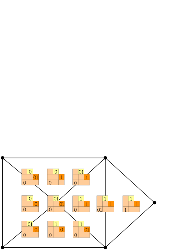
Figure 4. Continuing Example 1.6; the interior faces of the $2$-dimensional ${\rm KL}_{234651789\underline{10},\underline{10}954382761}$

The claims in Theorem 1.4 about the structure of ${\rm KL}_{v,w}$ then follow immediately from [KnuMilYon08, Theorem 2.8]. This was, we conclude that the interior faces of ${\rm KL}_{v,w}$ are labeled by semistandard set-valued drift tableaux while the exterior faces are labeled by non-semistandard but limit semistandard tableaux. Also the codimension of a face ${\mathcal{D}}$ is $|{\mathcal{D}}|-\#{\rm continents}$, the number of “extra” entries of ${\mathcal{D}}$.

4.2. $K$-polynomials of ${\rm KL}_{v,w}$

Let us take this opportunity to formalize a connection between the $K$-polynomials of ${\rm KL}_{v,w}$ and $P_{v,w}(q)$. We will utilize facts collected about general tableau complexes from [KnuMilYon08, Section 4]. Let $V$ be the set of vertices of a simplicial complex $\Delta$ and set $R=\Bbbk[\Delta]$ to be the polynomial ring in variables $x_{\mathfrak{v}}$ for ${\mathfrak{v}}\in V$. This is the ambient ring for the Stanley-Reisner ideal $I_{\Delta}=\left\langle\prod_{{\mathfrak{v}}\in F}x_{\mathfrak{v}}:F\mbox{\ is not a face of $\Delta$}\right\rangle$ of $\Delta$, and $R/I_{\Delta}$ is the Stanley-Reisner ring. We use the alphabet ${\bf t}_{\mathfrak{v}}=\{t_{\mathfrak{v}}:{\mathfrak{v}}\in V\}$ for the finely graded Hilbert series ${\rm Hilb}(R/I_{\Delta};{\bf t})$ and $K$-polynomials ${\mathcal{K}}(R/I_{\Delta},{\bf t})$.

Let us define a family of polynomials for $v\leq w$ where $w$ is covexillary. We will see this is a hybrid of the $K$-polynomial of ${\rm KL}_{v,w}$ and the Kazhdan-Lusztig polynomial $P_{v,w}(q)$:

(4.1) $${\mathfrak{P}}_{v,w}(\beta;{\bf t})=\sum_{{\mathcal{D}}\in SVDT(v,w)}\beta^{|{\mathcal{D}}|-\#{\rm continents}(v,w)}\prod_{b\in\lambda(w)}\prod_{y\in{\mathcal{D}}(b)}(1-t_{(b\not\mapsto y)}),$$

where $SVDT(v,w)$ is the set of set-valued drift tableaux associated to drift configurations in ${\rm drift}(v,w)$, $\#{\rm continents}(v,w)$ is the number of continents in ${\rm Pangaea}(v,w)$, $|{\mathcal{D}}|$ is the number of entries in ${\mathcal{D}}$. There are a number of interesting specializations of this polynomial. Here we do not assume $|{\mathcal{E}}_{v,w}(b)|>1$, i.e., $(b\not\mapsto y)$ might be a phantom vertex.

By the ballness/sphereness claim of ${\rm KL}_{v,w}$ from Theorem 1.4, together with [KnuMilYon08, Theorem 4.3] it follows that

(4.2) $${\mathfrak{P}}_{v,w}(-1;{\bf t})={\mathcal{K}}(R/I_{{\rm KL_{v,w}}};{\bf t})$$

One can consider a vertex decomposition of any complex $\Delta$ at a vertex ${\mathfrak{v}}$. This is given by $\Delta={\rm del}_{\mathfrak{v}}(\Delta)\cup{\rm star}_{\mathfrak{v}}(\Delta)$ where ${\rm del}_{\mathfrak{v}}(\Delta)=\{F\in\Delta:{\mathfrak{v}}\not\in F\}$ is the deletion of ${\mathfrak{v}}$ and ${\rm star}_{\mathfrak{v}}(\Delta)=\{F\in\Delta:F\cup\{{\mathfrak{v}}\}\in\Delta\}$ is the star of ${\mathfrak{v}}$. Automatically one has, for ${\mathfrak{v}}=(b\not\mapsto y)$

(4.3) $${\mathcal{K}}(R/I_{{\rm KL}_{v,w}};{\bf t})=t_{(b\not\mapsto y)}{\mathcal{K}}(R/I_{{\rm del}_{(b\not\mapsto y)}({\rm KL}_{v,w})};{\bf t})+(1-t_{(b\not\mapsto y)}){\mathcal{K}}(R/I_{{\rm star}_{(b\not\mapsto y)}({\rm KL}_{v,w})};{\bf t}).$$

By tracing the specializations below, one should eventually interpret recursions from [LasSch81] for $P_{v,w}(q)$ using (4.3) and thus vertex decompositions of ${\rm KL}_{v,w}$. We do not pursue this here.

Consider

(4.4) $${\mathfrak{P}}_{v,w}(-1;t_{(b\not\mapsto y)}\mapsto 1-x_{y})=\sum_{{\mathcal{D}}\in SVDT(v,w)}(-1)^{|{\mathcal{D}}|-\#{\rm continents}(v,w)}{\bf x}^{\mathcal{D}},$$

where

$${\bf x}^{\mathcal{D}}=\prod_{i\geq 0}x_{i}^{\tiny{\#\mbox{$i$'s appearing in ${\mathcal{D}}$}}}.$$

Another specialization is given by

(4.5) $${\mathfrak{P}}_{v,w}(0;t_{(b\not\mapsto y)}\mapsto 1-x_{y})=\sum_{{\mathcal{D}}\in SSDT(v,w)}{\bf x}^{\mathcal{D}},$$

where $SSDT(v,w)$ is the set of ordinary, semistandard drift tableau associated to $v,w$. (In setting $\beta=0$ we take the convention that $0^{0}=1$ in (4.1).)

Finally, by considering the principal specialization of (4.5) we have

$${\mathfrak{P}}_{v,w}(0;t_{(b\not\mapsto y)}\mapsto 1-q^{y})=P_{v,w}(q).$$

5. The proof of Theorem 1.4(I)

5.1. Proof of $Q_{v,w}(q)=P_{v,w}(q)$

We give a weight-preserving bijection between ${\rm drift}(v,w)$ and the trees weight-enumerated by Lascoux’s rule [Las95] for $P_{v,w}(q)$. We mostly follow the presentation of his rule found in [BilLak01, 6.3.29].

Given $\mathcal{D}\in{\rm drift}(v,w)$, construct a rooted, edge-labeled tree ${\mathcal{T}}$ as follows. Associate to each continent $C$ a non-root vertex of ${\mathcal{T}}$. Moreover if the special box $b$ of $C$ is southwest of the special box $b^{\prime}$ of an adjacent continent $C^{\prime}$, then we draw an edge between the corresponding vertices. If there is no special box strictly southwest of $b$, then the corresponding vertex is joined to the root of ${\mathcal{T}}$.

Thus, each $1\times 1$ continent $C=\{(h,\lambda(w)_{h})\}$ (equivalently, those that come from northeast corners of $\lambda(w)$) corresponds to a leaf $p$ of ${\mathcal{T}}$. Now we bound the edge incident to $p$ by $b_{h}-h$, where

$$b_{h}=\max\{m\ |\ B(v,w)_{m}\geq\lambda(w)_{h}+m-h\}.$$

Let $DL({\mathcal{T}})$ be the set of all edge labelings of ${\mathcal{T}}$ by nonnegative integers such that the labels weakly increase from root to leaf. For any edge labeled tree ${\mathcal{G}}$ let $|{\mathcal{G}}|$ be the sum of the edge labels of ${\mathcal{G}}$.

For example, below are the trees for drift configurations in Figure 3. The framed number below each leaf is the bound for that leaf.

Figure 5. Edge labeled trees from $DL({\mathcal{T}})=EL({\mathcal{T}})$, respectively corresponding to drift configurations in Figure 3.

Lemma 5.1.

There is a bijection $\Phi:{\rm drift}(v,w)\to DL({\mathcal{T}})$ such that ${\rm wt}({\mathcal{D}})=|\Phi({\mathcal{D}})|$.

Proof.

Define $\Phi({\mathcal{D}})$ to be the edge labeling of ${\mathcal{T}}$ such that the edge associated to a continent $C$ (i.e., the edge whose child end is the vertex associated to $C$) is labeled by the distance that $C$ has drifted in ${\mathcal{D}}$. That the labels are weakly increasing in $\Phi({\mathcal{D}})$ is implied by the condition that the continents do not overlap in ${\mathcal{D}}$. Note that if $C$ is a $1\times 1$ continent then $b_{h}-h$ is the largest distance that $C$ can drift inside $B(v,w)$; this accounts for the leaf bound (see Figure 5 for a diagram). It is then easy to check that $\Phi$ is the desired bijection. ∎

Lascoux’s rule constructs a tree ${\mathcal{T}}^{\prime}$ as follows: For the partition $\lambda(w)$, the parenthesis-word is a word using “(” and “)” and obtained by walking with east and south steps along the northeast border of $\lambda(w)$. We record a “(” for each east step and a “)” for each south step. Now pair left and right parentheses starting from the the closest pairs “$()$”. Each pair corresponds to a vertex of the tree, the closest pairs are associated to leaves and a pair encloses its children. Unpaired parentheses do not contribute to the tree. This process results in a directed forest. Finally, we introduce an additional root and attach an edge to the root of each tree in the forest.

Lemma 5.2.

There is a graph isomorphism $\delta:{\mathcal{T}}\to{\mathcal{T}}^{\prime}$. Moreover under this isomorphism if $v$ corresponds to a $1\times 1$ continent associated to a corner $c$ of $\lambda(w)$, then $\delta(v)$ corresponds to a closest parenthesis pair associated to the same corner $c$.

Proof.

Each leaf of ${\mathcal{T}}$ corresponds to a corner $c$ of $\lambda(w)$. On the other hand, this corner gives rise to a closest pair “$(\ )$” in Lascoux’s construction, which corresponds to a leaf of ${\mathcal{T}}^{\prime}$. Thus we can construct a bijection between the leaves of the two trees, which we now argue extends to the bijection $\delta$ between the two trees themselves.

A continent $C$ is a $z$-continent if it is defined by a $z$-special box $b$. Fix a vertex $v\in{\mathcal{T}}$ associated to such a continent. By construction, each child of $v$ is a vertex $\{v^{\prime}\}$ associated to a $y$-continent $C^{\prime}$ adjacent and northeast of $C$ in ${\rm Pangaea}(v,w)$, where $y<z$. Since $b\in C$ is a special box, by using the fact that $|{\rm arm}(b)|=|{\rm leg}(b)|$ we have that the column $b$ is in corresponds to a $($ and the row $b$ in in corresponds to a $)$ where these two parentheses are paired with one another in the parenthesis word. Clearly, this pair gives a vertex $v^{\prime}\in{\mathcal{T}^{\prime}}$, and all vertices of ${\mathcal{T}^{\prime}}$ arise this way. That is, there is a bijection at the level of vertices $\delta:{\mathcal{T}}\to{\mathcal{T}}^{\prime}$. Moreover, that the children of $\delta(v)$ are exactly $\{\delta(v^{\prime})\}$ (for children $v^{\prime}$ of $v$) is also immediate from the constructions of ${\mathcal{T}}$ and ${\mathcal{T}}^{\prime}$ ∎

Lascoux’s rule similarly defines increasing edge labelings $EL({\mathcal{T}})$ on ${\mathcal{T}}$ as we did for $DL({\mathcal{T}})$. It remains to check that these labelings are the same as the ones in $DL({\mathcal{T}})$. For this, we only need to show that the bound attached to the leaves are the same. In [BilLak01, 6.3.29, Step 2], for each given leaf, a bigrassmannian permutation is determined in three sub-steps, from which Lascoux’s leaf bounds are determined. We now explain these steps. (For readers comparing what follows with [BilLak01], note their $x$ is our ${\widetilde{w}}=w^{-1}w_{0}$ while their $w$ is our ${\widetilde{v}}=v^{-1}w_{0}$.)

The reader may find the following diagram useful for the description of Lascoux’s labeling process:

Figure 6. Diagram for the proof of $P_{v,w}(q)=Q_{v,w}(q)$

Sub-step (1) [leaves $p$ of ${\mathcal{T}}$ correspond to distinct numbers in the code of $\widetilde{w}$]: The code $(c_{1},\dots,c_{n})$ of $\widetilde{w}$ is given by

$$c_{i}=\#\{j>i\ |\ {\widetilde{w}}_{j}<{\widetilde{w}}_{i}\}=\#\{\mbox{boxes of $D(w)$ in row $i$}\}.$$

Recall $\lambda(w)$ is the result of sorting this code into decreasing order. A leaf $p$ of ${\mathcal{T}}$ corresponds to a corner ${\mathfrak{e}}^{\prime\prime}=(h,\lambda(w)_{h})$ of $\lambda(w)$. Associate $\lambda(w)_{h}$ to $p$. This $\lambda(w)_{h}$ is equal to $c_{i}$ for some $i$. Clearly a different $c_{i}$ is assigned to each $p$.

Sub-step (2) [$\lambda(w)_{h}$ gives a crossing of $\widetilde{w}$]: By definition, a crossing of $\widetilde{w}$ is a 4-tuple $(i,j,j+1,k)$ satisfying

(5.1) $$\widetilde{w}_{j+1}\leq\widetilde{w}_{k}<\widetilde{w}_{i}\leq\widetilde{w}_{j},\quad\widetilde{w}_{i}=\widetilde{w}_{k}+1\mbox{\quad for $i\leq j<k$;}$$

cf. [LasSch96]. Now given the ${\mathfrak{e}}^{\prime\prime}$ associated to $p$, there is a unique essential box ${\mathfrak{e}}$ in $D(w)$ that is diagonally northeast of ${\mathfrak{e}}^{\prime\prime}$. We define $j$ and $k$ by declaring that the coordinates of ${\mathfrak{e}}$ are $(j,{\widetilde{w}}_{k})$. Let $i$ be such that $\widetilde{w}_{i}=\widetilde{w}_{k}+1$.

We claim that $(i,j,j+1,k)$ forms a crossing. Let us first check the weak inequalities of $\widetilde{w}_{j+1}\leq\widetilde{w}_{k}<\widetilde{w}_{i}\leq\widetilde{w}_{j}$ (the strict inequality being true by definition). For the rightmost inequality, we have ${\widetilde{w}}_{j}=w^{-1}w_{0}(j)=w^{-1}_{n-j+1}$, which in words is the column position of the $\bullet$ of $G(w)$ that necessarily must be to the right of ${\mathfrak{e}}$, which itself is in column ${\widetilde{w}}_{k}$. In other words ${\widetilde{w}}_{k}\leq{\widetilde{w}}_{j}$. Now, for the leftmost inequality, note ${\widetilde{w}}_{j+1}=w^{-1}w_{0}(j+1)=w^{-1}(n-j)$ which is the column position of the $\bullet$ of $G(w)$ in row $j+1$. Since ${\mathfrak{e}}$ is an essential box, that $\bullet$ must be weakly to the left, i.e., ${\widetilde{w}}_{j+1}\leq{\widetilde{w}}_{k}$, as desired. It remains to check $i\leq j$ and $j<k$. For the former inequality, we compute $w{\widetilde{w}}_{i}=n-i+1$ which is the row position of the $\bullet$ of $G(w)$ in column ${\widetilde{w}}_{i}$. Since ${\mathfrak{e}}$ is an essential box, the $\bullet$ is weakly below the ${\mathfrak{e}}$, i.e., $i\leq j$. Similarly, for the latter inequality, we consider $w{\widetilde{w}}_{k}=n-k+1$, which is the position of the $\bullet$ of $G(w)$ in column ${\widetilde{w}}_{k}$. This must be strictly above the ${\mathfrak{e}}$, i.e., $j<k$.

Now associate the crossing $(i,j,j+1,k)$ to $p$ (and hence $\lambda(w)_{h}$). Actually, the description in [BilLak01] gives a different way to assign a crossing to $p$. However, it is straightforward to check that their crossing is same as the one described above.

Sub-step (3) [each crossing gives a maximal bigrassmannian $[a,b,c,d]$ below $\widetilde{w}$]: Here $[a,b,c,d]$ denotes

$$(1,\dots,a,a+c+1,\dots,a+c+b,a+1,\dots,a+c,a+c+b+1,\dots,a+b+c+d)\in S_{n}.$$

Lascoux’s rule corresponds $(i,j,j+1,k)$ to a maximal bigrassmannian

$$[z,j-z,{\widetilde{w}}_{k}-z,n-{\widetilde{w}}_{k}-j+z],$$

where

$$z=\#\{p<j:{\widetilde{w}}_{p}<{\widetilde{w}}_{k}\}.$$

Notice $z$ is the number of $\bullet$’s in $G(w)$ weakly southwest of ${\mathfrak{e}}=(j,{\widetilde{w}}_{k})$, i.e.

(5.2) $$z=r^{w}_{\mathfrak{e}}.$$

This concludes Sub-step (3) of step 2 of [BilLak01].

Lascoux’s rule then assigns to $p$ the following leaf bound:

$${\rm distance}([z,j-z,{\widetilde{w}}_{k}-z,n-{\widetilde{w}}_{k}-j+z],\widetilde{v}),$$

where

$${\rm distance}([a,b,c,d],\widetilde{v})=\max\{r\geq 0|[a-r,b+r,c+r,d-r]\leq\widetilde{v}\,\},$$

and where “$\leq$” refers to Bruhat order on $S_{n}$.

This completes the description of Lascoux’s algorithm.

Recall $r^{v}_{(a+b,a+c)}$ equals the number of dots of $G(v)$ weakly southwest of $(a+b,a+c)$. Observe the following fact, whose proof is straightforward to argue (and also follows from the deeper developments in [LasSch96]):

Lemma 5.3.

For any bigrassmannian permutation $[a,b,c,d]$ and permutation $\widetilde{v}$ in $S_{n}$, the inequality $[a,b,c,d]\leq\widetilde{v}$ is equivalent to $r^{v}_{(a+b,a+c)}\leq a$, where $v=w_{0}\widetilde{v}^{-1}$.∎

Proposition 5.4.

The leaf bounds on $DL({\mathcal{T}})$ and $EL({\mathcal{T}})$ are the same.

Proof.

By Lemma 5.3,

(5.3) $$[z-r,j-z+r,{\widetilde{w}}_{k}-z+r,n-{\widetilde{w}}_{k}-j+z-r]\leq\widetilde{v}$$

$$\iff r^{v}_{(z-r)+(j-z+r),(z-r)+({\widetilde{w}}_{k}-z+r)}\leq z-r$$

$$\iff r^{v}_{(j,{\widetilde{w}}_{k})}\leq z-r$$

$$\iff r^{v}_{{\mathfrak{e}}}\leq z-r.$$

Hence, the maximal $r$ such that any of the inequalities (5.3) hold is

$$r=z-r^{v}_{{\mathfrak{e}}}=r^{w}_{{\mathfrak{e}}}-r^{v}_{{\mathfrak{e}}},$$

where we have used (5.2).

In terms of drift configurations, $r$ is the largest distance that a corner ${\mathfrak{e}}^{\prime\prime}=(h,\lambda(w)_{h})$ can be moved diagonally northeast and remain in $B(v,w)$ (cf. [LiYon10, Lemma 5.7]). By the definition of $B(v,w)$, $b_{h}=j-r^{v}_{\mathfrak{e}}$. It is also easy to check that $j=h+r^{w}_{\mathfrak{e}}$ (again by [LiYon10, Lemma 5.7]). Then

$$b_{h}-h=j-r^{v}_{\mathfrak{e}}-h=(j-h)-r^{v}_{\mathfrak{e}}=r^{w}_{\mathfrak{e}}-r^{v}_{\mathfrak{e}}=r.$$

This completes the proof of the proposition. ∎

By Lascoux’s rule,

$$P_{w_{0}{\widetilde{v}},w_{0}{\widetilde{w}}}(q)(=P_{w_{0}v^{-1}w_{0},w_{0}w^{-1}w_{0}}(q)=P_{v,w}(q))=\sum q^{|T|}$$

where the sum is over $EL(T)$ and $|T|$ is the total sum of the edge labels. Since we have established the desired weight-preserving bijection, the claim $Q_{v,q}(q)=P_{v,w}(q)$ then follows.

Remark 5.5.

There are two basic symmetries of the Kazhdan-Lusztig polynomials: (1) $P_{v,w}(q)=P_{w_{0}v^{-1}w_{0},w_{0}w^{-1}w_{0}}(q)$ and (2) $P_{v,w}(q)=P_{v^{-1},w^{-1}}(q)$. The symmetry (1) is manifest in our rule and ${\rm drift}(w_{0}vw_{0},w_{0}ww_{0})$ is obtained by transposing the drift configurations of ${\rm drift}(v,w)$. For (2), it is an exercise to prove that $\lambda(w)=\lambda(w^{-1})$ and $B(v,w)=B(v^{-1},w^{-1})$ and so ${\rm drift}(v^{-1},w^{-1})={\rm drift}(v,w)$.

Remark 5.6.

From Theorem 1.4(I) it is not hard to show the following. For $w,v\in S_{n}$ where $w$ is covexillary and $v\leq w$, let $k$ be the number of special boxes of $\lambda(w)$ and let $m=\lfloor\frac{n-k+1}{2}\rfloor$. If $[m]_{q}=1+q+\cdots+q^{m-1}$, then $[q^{i}]P_{v,w}(q)\leq[q^{i}]([m]_{q})^{k}$ for all $i$. In particular, $P_{v,w}(1)\leq m^{k}$.

6. Another $q$-analogue of multiplicity

We can think of $H_{v,w}(q)$ as a $q$-analogue of Hilbert-Samuel multiplicity, in the sense that $H_{v,w}(1)={\rm mult}_{e_{v}}(X_{w})$. Let us point out that in the covexillary setting, there is another $q$-analogue available. As in Theorem 1.4(II), regard each box of $\lambda(w)$ as a separate country; the “drift configurations” are precisely the pipe dreams $P\in{\rm Pipes}(v,w)$ in [LiYon10]. Now let

$${\widetilde{\rm wt}}(P)=q^{d}$$

where $d$ is the total of the distance drifted by the countries, and set

$${\widetilde{H}}_{v,w}(q)=\sum_{\rm P\in{\rm Pipes}(v,w)}{\widetilde{\rm wt}}(P).$$

In the following theorem we use the standard $q$-notation:

$$[a]_{q}=1+q+\cdots+q^{a-1}\mbox{\ and ${a\choose b}_{q}=\frac{[a]_{q}[a-1]_{q}\cdots[a-b+1]_{q}}{[b]_{q}\cdots[1]_{q}}$.}$$

Theorem 6.1.

$${\widetilde{H}}_{v,w}(q)=q^{-\sum_{i\geq 1}(i-1)\lambda_{i}}\det\left({b_{i}+\lambda_{i}-i+j-1\choose\lambda_{i}-i+j}_{q}\right)_{1\leq i,j\leq\ell(\lambda)},$$

where $\ell(\lambda)$ is the number of nonzero parts of $\lambda$ and ${\bf b}={\bf b}(\Theta_{v,w})$.

Proof.

For brevity, we refer the reader to the setup of [LiYon10, Sections 5.2 and 6.2]. Notice that

$$s_{\lambda,{\bf b}}(1,q,q^{2},q^{3},\ldots)=\det\left({b_{i}+\lambda_{i}-i+j-1\choose\lambda_{i}-i+j}_{q}\right)_{1\leq i,j\leq\ell(\lambda)}$$

where the lefthand side of the equality is the principal specialization of the (single) flagged Schur polynomial for shape $\lambda(w)$ with flag ${\bf b}={\bf b}(\Theta_{v,w})$.

Given a pipe dream $P\in{\rm Pipes}(v,w)$ that corresponds to a flagged semistandard Young tableau $T$, write

$${\rm wt}_{x}(P):={\rm wt}_{x}(T)$$

to mean the usual multivariate weight assigned to $T$ (i.e., so that $s_{\lambda,{\bf b}}(x_{1},x_{2},x_{3},\ldots)=\sum_{T}{\rm wt}_{x}(T)$). Let ${\rm wt}_{q}^{\prime}(P)$ be the principal specialization of ${\rm wt}_{x}(P)$ given by $x_{i}\mapsto q^{i-1}$ and finally set

$${\rm wt}_{q}(P)=q^{-\sum_{i\geq 1}(i-1)\lambda_{i}}\times{\rm wt}_{q}^{\prime}(P).$$

It remains to show that for each $P$, ${\rm wt}_{q}(P)={\widetilde{\rm wt}}(P)$. To do this, let us induct on ${\widetilde{\rm wt}}(P)\geq 0$. The base case that ${\widetilde{\rm wt}}(P)=0$, i.e., where $P$ is the starting configuration holds since ${\rm wt}^{\prime}_{q}(P)=q^{\sum_{i\geq 1}(i-1)\lambda_{i}}$.

Now suppose ${\widetilde{\rm wt}}(P)>0$. Then there is a $P^{\prime}$ such that a move of the form

$$\begin{matrix}\cdot&\cdot\\ +&\cdot\end{matrix}\ \ \mapsto\ \ \begin{matrix}\cdot&+\\ \cdot&\cdot\end{matrix}$$

in some $2\times 2$ subsquare of $[n]\times[n]$ brought us to $P$ (and no other $+$ in $P^{\prime}$ has changed). Thus, we can compare ${\rm wt}_{x}(P^{\prime})$ and ${\rm wt}_{x}(P)$: the latter only differs from the former in that some factor of $x_{i}$ changed to $x_{i+1}$ (where $i$ and $i+1$ are the rows changed by the move above). Hence applying induction we have

$${\rm wt}_{q}(P)={\rm wt}_{q}(P^{\prime})\times q={\widetilde{\rm wt}}(P^{\prime})\times q={\widetilde{\rm wt}}(P),$$

as desired. ∎

It is clear from Theorem 1.4 that

$$P_{v,w}(q)\preceq{\widetilde{H}}_{v,w}(q).$$

With the same proof that we used for $H_{v,w}(q)$, one shows that ${\widetilde{H}}_{v,w}(q)$ is upper semicontinuous. However, in general ${\widetilde{H}}_{v,w}(q)\neq H_{v,w}(q)$. Moreover, we do not know any algebraic/geometric measure for general Schubert varieties that specializes to ${\widetilde{H}}_{v,w}(q)$.

7. Concluding remarks

We are presently unaware of any geometric proof of the inequality of Theorem 1.2. For general $Y$, let us assume, for simplicity of our discussion, that all odd local intersection cohomology groups vanish, and set

$$P_{p,Y}(q)=\sum_{i\geq 0}\dim({\mathcal{H}}_{p}^{2i}(Y))q^{i}.$$

Question 7.1.

Under what assumptions is either the inequality $P_{p,Y}(q)\preceq H_{p,Y}(q)$ and/or the weaker inequality $P_{p,Y}(1)\leq H_{p,Y}(1)(={\rm mult}_{p}(Y))$ true?

Our results on $H_{v,w}(q)$ are based on the degeneration, flat over ${\rm Spec}({\mathbb{Z}})$, given in [LiYon10]. Hence Theorem 1.7 is valid over a field ${\Bbbk}$ of arbitrary characteristic and Conjecture 1.1 seems similarly valid. However, the arguments of [LiYon10] also prove that the projectivized tangent cones of the Kazhdan-Lusztig varieties ${\mathcal{N}}_{v,w}$ are isomorphic to those for ${\mathcal{N}}_{id,\Theta_{v,w}}$. It is then not hard to construct some cograssmannian $v^{\prime},w^{\prime}$ with the same property. We do not know if ${\mathcal{N}}_{v,w}$ and any such ${\mathcal{N}}_{v^{\prime},w^{\prime}}$ are actually isomorphic, although a number of useful implications would be a consequence of this fact.

A number of formulae have been obtained for $P_{v,w}(q)$. For example, general, non-positive formulae have been obtained by [BilBre07] and [Bre94]. Beyond the covexillary case, few positive formulae are known, see, e.g., [BilWar01] (which treats the $321$-hexagon avoiding case) and the references therein. It would be interesting to try to extend our main theorems to these other contexts as well.

Finally, we believe many of the ideas of this paper can be extended to other Lie groups. In particular, we expect Theorems 1.2, 1.4 and 1.7 to have analogues for (co)minuscule $G/P$, cf. [Boe88]. However, this requires sufficient technicalities that it is better left to a separate treatment.

References

- [BilBre07] L. Billera and F. Brenti, Quasisymmetric functions and Kazhdan-Lusztig polynomials, preprint 2007. arxiv:0710.3965
- [BilLak01] S. Billey and V. Lakshmibai, Singular loci of Schubert varieties, Progr. Math. 182(2000), Birkhäuser, Boston.
- [BilWar01] S. Billey and G. Warrington, Kazhdan-Lusztig polynomials for -hexagon-avoiding permutations, J. Alg. Comb., 13(2) (2001), 111–136.
- [Boe88] B. D. Boe, Kazhdan-Lusztig polynomials for hermitian symmetric spaces, Trans. Amer. Math. Soc. 309(1988), 279–294.
- [BraMac01] T. Braden and R. MacPherson, From moment graphs to intersection cohomology, Math. Ann. 321(2001), no. 3, 533–551.
- [Bre98] F. Brenti, Lattice paths and Kazhdan-Lusztig polynomials, J. Amer. Math. Soc., 11(1998), 229–259.
- [Bre94] by same author, Log-concave and unimodal sequences in algebra, combinatorics, and geometry: an update, Jerusalem combinatorics ’93, 71–89, Contemp. Math., 178, Amer. Math. Soc., Providence, RI, 1994.
- [Bri03] M. Brion, Lectures on the geometry of flag varieties, Notes de l’école d’été “Schubert Varieties” (Varsovie, 2003), 59 pages.
- [BruHer93] W. Bruns and J. Herzog, Cohen-Macaulay rings, Cambridge Studies in Advanced Mathematics, 39. Cambridge University Press, Cambridge, 1993. xii+403 pp.
- [Buc00] A. S. Buch, A Littlewood-Richardson rule for the -theory of Grassmannians, Acta Math. 189(2002), no. 1, 37–78.
- [Ful92] W. Fulton, Flags, Schubert polynomials, degeneracy loci, and determinantal formulas, Duke Math. J. 65 (1992), no. 3, 381–420.
- [IkeNar09] T. Ikeda and H. Naruse, Excited Young diagrams and equivariant Schubert calculus, Trans. Amer. Math. Soc. 361(2009), 5193–5221.
- [Irv88] R. Irving, The socle filtration of a Verma module, Ann. Sci. École. Norm. Sup. series 421(1988), no. 1, 47–65.
- [JonWoo10] B. Jones and A. Woo, Kazhdan-Lusztig polynomials for cograssmannian permutations, preprint, 2010.
- [KazLus80] D. Kazhdan and G. Lusztig, Schubert varieties and Poincaré duality, Proc. Symp. Pure. Math., A. M. S., 36(1980), 185–203.
- [KazLus79] by same author, Representations of Coxeter Groups and Hecke Algebras, Invent. Math. 53 (1979), 165–184.
- [Knu09] A. Knutson, Frobenius splitting, point counting, and degeneration, preprint, 2009. arXiv:0911.4941
- [KnuMil05] A. Knutson and E. Miller, Gröbner geometry of Schubert polynomials, Ann. of. Math. (2) 161(2005), no. 3, 1245–1318.
- [KnuMil04] by same author, Subword complexes in Coxeter groups, Adv. Math. 184(2004), no. 1, 161–176.
- [KnuMilYon09] A. Knutson, E. Miller and A. Yong, Gröbner geometry of vertex decompositions and of flagged tableaux, J. Reine Angew. Math. 630(2009), 1–31.
- [KnuMilYon08] by same author, Tableau complexes, Israel J. Math., 163(2008), 317–343.
- [KreRob05] M. Kreuzer, L. Robbiano, Computational commutative algebra. 2, Springer-Verlag, Berlin, 2005. x+586 pp.
- [LakSan90] V. Lakshmibai and B. Sandhya, Criterion for smoothness of Schubert varieties in , Proc. Indian Acad. Sci. Math. Sci. 100 (1990), no. 1, 45–52.
- [Las95] A. Lascoux, Polynomes de Kazhdan-Lusztig pour les varietes de Schubert vexillaires, C. R. Acad. Sci. Paris Ser. I Math. 321(6), (1995), 667 ड 1ऄ1 770.
- [LasSch96] A. Lascoux and M. -P. Schützenberger, Treillis et bases des groupes de Coxeter, Electron. J. Combin., 3:2 (1996).
- [LasSch81] by same author, Polynomes de Kazhdan Lusztig pour les Grassmanniennes, Astérisque 87–88 (1981), 249–266.
- [LiYon10] L. Li and A. Yong, Some degenerations of Kazhdan-Lusztig polynomials and multiplicities of Schubert varieties, preprint 2010. arXiv:1001.3437
- [Man01a] L. Manivel, Symmetric functions, Schubert polynomials and degeneracy loci, American Mathematical Society, Providence 2001.
- [Man01b] by same author, Generic singularities of Schubert varieties, preprint 2001. arXiv:math.AG/0105239.
- [MilStu04] E. Miller and B. Sturmfels, Combinatorial Commutative Algebra, Graduate Texts in Mathematics Vol. 227, Springer-Verlag, New York, 2004.
- [Pol00] P. Polo, Construction of arbitrary Kazhdan-Lusztig polynomials, Represent. Theory 3 (1999), 90–104.
- [Ram85] A. Ramanathan, Schubert varieties are arithmetically Cohen-Macaulay, Invent. Math., 80(1985), 283–294.
- [Rub05] M. Rubey, The -vector of a ladder determinantal ring cogenerated by minors is log-concave, J. Algebra 292(2005), no. 2, 303–323.
- [ShiZin10] K. Shigechi and P. Zinn-Justin, Path representation of maximal parabolic Kazhdan-Lusztig polynomials, preprint 2010. arXiv.1001.1080
- [Sta89a] R. P. Stanley, Log-concave and unimodal sequences in algebra, combinatorics, and geometry. Graph theory and its applications: East and West (Jinan, 1986), 500–535, Ann. New York Acad. Sci., 576, New York Acad. Sci., New York, 1989.
- [WooYon09] A. Woo and A. Yong, A Gröbner basis for Kazhdan-Lusztig ideals, preprint 2009. arxiv:0909.0564
- [WooYon08] by same author, Governing singularities of Schubert varieties, J. Algebra, 320(2008), no. 2, 495–520.