Relic Abundance Predicts Universal
Mass-Width Relations for Dark Matter Interactions

Abstract

We find new and universal relations for the properties of dark matter particles consistent with standard relic abundances. Analysis is based on first characterizing the $s$-channel resonant annihilation process in great detail, keeping track of all velocity-dependence, the presence of multiple scales and treating each physical regime above, below, and close to thresholds separately. The resonant regime as well as extension to include non-resonant processes are then reduced to analytic formulas and inequalities that describe the full range of multi-dimensional numerical work. These results eliminate the need to recompute relic abundance model by model, and reduce calculations to verifying certain scale and parameter combinations are consistent. Remarkably simple formulas describe the relation between the total width of an $s$-channel intermediate particle, the masses and the couplings involved. Eliminating the width in terms of the mass produces new consistency relations between dark matter masses and the intermediate masses. The formulas are general enough to test directly whether new particles can be identified as dark matter. Resonance mass and total width are quantities directly observable at accelerators such as the LHC, and will be sufficient to establish whether new discoveries are consistent with the cosmological bounds on dark matter.

Thermal evolution of dark matter in the early universe can be found in textbooks to predict a velocity-averaged annihilation cross section ${\langle\sigma v\rangle}\sim 3\times 10^{-26}cm^{3}/s$. However the textbook exercise happens to assume velocity-independent cross sections that are neither general, nor reliable. In this paper we give a complete and general analysis based on a new strategy. Our method solves the inverse problem of bounding the multi-dimensional parameter regions such that the relic abundance is fixed. The analysis involves several novel steps.

Many models are summarized by $t$ and $u$-channel exchanges that are slowly varying, plus $s$-channel resonances that are a great complication. An early study by Greist and Seckel griest noted that resonant processes violate the assumptions of constant cross sections, while being impossible to summarize with equivalently simple formulas. A typical resonant calculation involves several coupling constants and 5 dimensionful scales: the incoming energy, two masses $m_{X}$, $m_{Y}$, the final state mass or masses, and the final relic density. Choosing one point in this huge parameter space and solving the Boltzmann relic evolution will predict one particular relic density. Complete exploration has previously appeared impossible, and most studies are limited to checking consistency in a plane of a few selected parameters.

Our approach first characterizes relic evolution via $s$-channel annihilation. The work is partly numerical, and partly analytic; we make no assumptions about masses, couplings, or final states. We find several tricks to identify the important scales and ratios of scales that describe every possible parameter region. We use unitarity and the optical theorem to represent exactly the $s$-channel decay into all possible final states.

As a result, we find universal mass-width relations which fit the numerical work across the whole parameter range. Let $X$ be the dark matter (mass $m_{X})$, and $Y$ be the $s$-channel intermediate connector (mass $m_{Y}$, width $\Gamma_{Y})$, by which $X+X\rightarrow Y\rightarrow anything$. The mass-v-width relation for the pole below threshold is

$$\Gamma_{Y}(m_{Y}<2m_{X}) = {8\over\pi}{1\,GeV\over C_{jj^{\prime}}\alpha_{XXY}}\left({m_{X}\over 730\,GeV}\right)^{3}$$

$$\times\left(1+{m_{X}\over 2m_{Y}}\right)\left(1-\frac{m_{Y}}{2m_{X}}\right)^{2}.$$

Here $\alpha_{XXY}$ is the coupling of dark matter to the intermediate connector particle, and $C_{jj^{\prime}}$ is a spin-counting coefficient from which dimensionful scales have been removed. An equivalent formula for a pole above threshold ($m_{Y}>2m_{X}$) is presented in Eq. 16, Section IV.

To show how the relation works, suppose an $s$-channel connector of mass $m_{Y}=600$ GeV has coupling $\alpha_{XYY}=10^{-2}$ and width $\Gamma_{Y}=5$ GeV. Then $m_{X}=417.8$ GeV is the mass of the dark matter if the pole lies below threshold and dominates the relic evolution. This is far more precise and specific than the order-of-magnitude estimates generated by ${\langle\sigma v\rangle}\sim 3\times 10^{-26}cm^{3}/s$. If we have the same mass $m_{X}$, and the width $\Gamma_{Y}=2$ GeV, then the resonance $Y$ is too narrow to give the usual relic abundance.

Many examples of dominant $s$-channel dark matter annihilation models can be found in the literature Ibe:2009dx ; Kadota:2010xm . However we are not limited to $s$-channel dominance. The most general cross section, including any number of channels and interference, is either larger or smaller than the $s$-channel annihilation. Supposing that the cross section with extra non-resonant channels is larger provides an inequality of a particular sense, given in Section II.2. An inequality of the opposite sense comes from the opposite assumption. In general the $s$-channel dominant case produces a bounding surface in the space of all the parameters. The surface is simple enough that a number of powerful inequalities in selected parameter planes come out rather easily. But we can do more: Eq. LABEL:newanappx shows quantitatively how to take into account any amount of resonant versus non-resonant cross sections with a simple “replacement rule.”

The mass-width relations also serve as a test of any new physics compared to dark matter cosmology. If the width and mass of a resonance do not match our relations then it is not a candidate to produce relics. Conversely a match of mass and width would be an indisputable signal of discovery. Note the width of a new particle is always a physical observable available from its production, allowing direct data-versus-data comparisons not depending on model details. Thus we expect our formulas to be useful for dark matter studies at the LHC and the ILC Cheung:2007ut ; Kumar:2006gm ; Han:2007ae .

Moreover, widths are calculable in almost every model. The ansatz $\Gamma_{Y}=\alpha_{\Gamma}m_{Y}$ is typical, but we also use it as a definition of the symbol $\alpha_{\Gamma}$ for analysis. Recall that the Standard Model $Z$-boson has a mass of $m_{Z}=91.2GeV$ and a total width $\Gamma_{Z}=2.1GeV$, giving an effective coupling of $\alpha_{Z}=0.03$. The effective coupling absorbs all the channels, including the invisible ones, all the couplings, spin factors, and phase space. Combining $\Gamma_{Y}=\alpha_{\Gamma}m_{Y}$ with Eq. ‣ Relic Abundance Predicts Universal Mass-Width Relations for Dark Matter Interactions yields a non-linear equation relating $m_{X}$, $m_{Y}$ and the couplings. For $m_{X}>>100$ GeV the relation reduces to $m_{Y}=2m_{X}+c_{1}+c_{2}/m_{X}+...$ where $c_{1}$, $c_{2}$ are known functions of couplings. It is very surprising there is always an allowed solution for arbitrarily large $m_{X}$, $m_{Y}$, contrary to the expectations of Born-level estimates. In the event that symbol $\alpha_{\Gamma}$ contains some mass dependence, as with certain theories with dimensionful couplings, the mass relation remains good and can be explored without needing to repeat the relic abundance calculations.

We built on previous experience with $s$-channel annihilation effects in the galactic halo Backovic:2009rw . Velocity dependence in annihilation came to the front with recent satellite data from PAMELA Adriani:2008zr , FERMI Baltz:2008wd , PPB-BETS Torii:2008xu and other experiments Barwick ; chang . Whether or not the data might be a signal, the studies have led to recognition that Born-level cross sections are not adequate. Exaggerated claims about “Sommerfeld factors,” sometimes thought to be exact non-perturbative effects, both violate general principles Backovic:2009rw and phenomenological tests Dent:2009bv ; Zavala:2009mi ; Feng:2010zp . Refs. haloIbe ; haloGuo ; Backovic:2009rw found the enhancements of ordinary resonant physics can be surprisingly large. Resonant processes can saturate unitarity bounds on annihilation in halo circumstances, generating large “boost factors” suggested by the data. It is because certain width-dependent effects ,perturbatively small in the high energy limit, may dominate everything in the non-relativistic limit. The problems of hevy thremal relic evolution in the early universe are similar, because the abundance is determined primarily in a regime sensitive to non-relativistic dynamics. Refs. Baro:2007em ; Drees:2009gt show concrete examples in which even the effects of one loop corrections on the relic abundance can be significant.

There are many applications of our results. Section I reviews the standard relic abundance formalism for completeness. Section II presents the $s$-channel mass-width relation for a pole below threshold, along with motivation for the analytic formula. At each stage where it is appropriate we convert the equalities developed for $s$-channel dominance into inequalities, illustrated with graphics. Section III explores consequences of calculable widths. This leads to $m_{X}-m_{Y}$ relations between the intermediate particle and the dark matter. The surprising fact that $m_{Y}\sim 2m_{X}$ can fit relic abundance for arbitrarily large masses is something to explore. It turns out to be a generalization of the “funnel’ region” known in minimal supersymmetric models (SUSY) Bhattacharya:2009ij ; Djouadi:2005dz ; Ellis:2007by ; Lahanas:2001yr ; Herrmann:2007ku ; Belanger:2006qa , without making an assumption of SUSY. We suspect that our relations are more restrictive than the commonly known ones, and may rule out some models. Separate analysis for the case where the intermediate connector mass $m_{Y}$ is above the kinematic threshold $2m_{X}$ is given in Section IV.

I Cross Sections and Relic Abundance

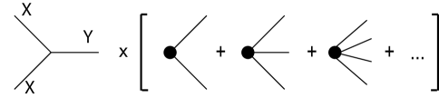
Figure 1: $s$-channel dark matter annihilation diagrams into all possible final states.

The thermally evolving number density $Y$ is calculated as a function of the inverse temperature $x\equiv m_{X}/T$ using

$$\frac{dY}{dx}=\xi(x,\,m_{X}){\langle\sigma v\rangle}(x)(Y^{2}-Y^{2}_{EQ}),$$

where $Y_{EQ}$ is the equilibrium density, and $\xi(x,\,m_{X})=-xs(x)/H(m_{X})$ is a combination of standard entropy and Hubble functions Kolb . The asymptotic solution follows in the regime of $Y_{EQ}\rightarrow 0$:

$$\frac{dY}{Y^{2}} = \xi(x,\,m_{X}){\langle\sigma v\rangle}(x)dx;$$

$$Y_{\infty}^{-1} = \int_{x_{d}}^{\infty}dx\,\xi(x,\,m_{X}){\langle\sigma v\rangle}.$$ (1)

The lower limit $x_{d}$ is computed self-consistently. Given the standard value of the critical density, the asymptotic density $\Omega=m_{X}Y_{\infty}s_{0}/\rho_{crit}$ follows, using the critical density $\rho_{crit}$ and entropy density $s_{0}$ of the present universe.

Particle physics enters in the annihilation cross section $\sigma(v)$ and its thermal average ${\langle\sigma v\rangle}(x)$. The rapid energy dependence and multiple scales of resonant cross sections require special analysis. Expansions of the form ${\langle\sigma v\rangle}\approx a+b/x+c/x^{2}+...$ are never good approximations over the entire range of $x$.

Let $M_{XX\rightarrow f}$ be the amplitude for $XX$ to go to a final state $f$. The cross section $\sigma$ goes like the amplitude-squared, summed over all final states (Fig.1), and integrated over final state phase space LIPS:

$$d\sigma\sim{1\over flux}\sum_{f}\,|M_{XX\rightarrow f}|^{2}\,dLIPS.$$

The total cross section into all possible final states is given by the optical theorem:

$$\sigma_{tot}=-{1\over 2kE_{CM}}Im(M(s,\,t=0)).$$

Here $k$ is the momentum of either particle in the center of mass frame, and $M$ is the elastic scattering amplitude. For a given total center of mass energy $E_{CM}$ and its square $s$, the forward propagators of intermediate states $Y$ go like $(s-m_{Y}^{2}+im_{Y}\Gamma)^{-1}$, where $\Gamma$ is the total width. Let $g_{XXY}^{2}t_{jj^{\prime}}$ be the component of the elastic amplitude containing the couplings of the initial/final states of spin $j$ to an $s$-channel particle of spin $j^{\prime}$. Then channel by channel, the optical theorem predicts

$$\sigma_{tot} = -{1\over 2kE_{CM}}Im\left({g_{XXY}^{2}t_{jj^{\prime}}\over s-m_{Y}^{2}+im_{Y}\Gamma_{Y}}\right)$$ (2)

$$= {g_{XXY}^{2}\over 2kE_{CM}}{m_{Y}\Gamma_{Y}t_{jj^{\prime}}\over(s-m_{Y}^{2})^{2}+m_{Y}^{2}\Gamma_{Y}^{2}}.$$

The symbol $\Gamma_{Y}$ represents the total width of $Y$ to all final states, which allows us to describe numerous models with a single parameter.

In standard convention for amplitudes, the Feynman rules contain in/out state polarization and vertex factors compiled into the symbol $t_{jj^{\prime}}$. It is important to extract the mass ($m_{X})$ dependence of these factors for analysis. We define

$$t_{jj^{\prime}}=4m_{X}^{2}C_{jj^{\prime}},$$ (3)

whereby $C_{jj^{\prime}}$ is typically a number of order unity. Scaling like $m_{X}^{2}$ is expected from dimensional analysis, and inevitable when the initial state is dominated by the mass as the largest scale. We emphasize that $C_{jj^{\prime}}$ is a definition that allows for any model while postponing spin-sums and vertex factors until a model is chosen. For example, the annihilation of unpolarized Dirac Fermions via a $\gamma^{\mu}$ vertex produces $C_{{1/2}\,1}=3/4.$ Another example is the annihilation of two scalar particles to a vector, which will have two derivatives going like $k^{2}\sim m_{X}^{2}$, times the polarization sum over the vector particle modes. The coupling and spin factors then appear in the combination $4\pi a_{XXY}C_{jj^{\prime}}$, where $\alpha_{XYY}=g_{XXY}^{2}/(4\pi)$.

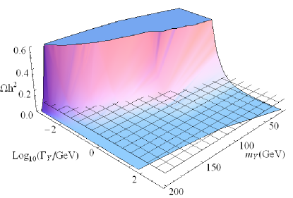
Figure 2: Intersection of the mesh plane representing $\Omega h^{2}=0.1$ and the surface $\Omega h^{2}(\Gamma_{Y},m_{Y},m_{*},\alpha_{*})$ gives a unique curve $\Gamma(m_{Y})$. $m_{*}=100GeV$, $\alpha_{*}=0.01$ for the purpose of the graphic.

Now all $m_{X}$ dependence of the cross section, rate ${\langle\sigma v\rangle}$, and density $Y_{\infty}$ dependence has been scaled out, except for a minor cutoff ($x_{d}$) dependence in Eq. 1, which must be reconciled numerically. In the numerical work we first choose a particular dark matter mass $m_{X}=m_{*}$ and coupling $\alpha_{*}$, and then compute thousands of relic densities covering the $\Gamma_{Y}$, $m_{Y}$ plane. The condition $\Omega(\Gamma_{Y},\,\,m_{*},\,m_{Y},\alpha_{*})h^{2}\rightarrow 0.1$ produces a unique curve $\Gamma_{Y}$ versus $m_{Y}$, namely the function $\Gamma_{Y}=\Gamma_{Y}(m_{Y};\,m_{*},\alpha_{*})$, as seen in Fig. 2. With the scaling relations in hand, the curves are extended to numerical predictions for the general functional dependence of $\Gamma=\Gamma(m_{Y};\,m_{X},\alpha_{XYY})$ consistent with a fixed relic density.

II Mass-Width Relations: Pole Below Threshold ($m_{Y}<2m_{X}$)

Fig. 3 shows the mass-width relation as a family of curves plotted for selected $m_{X}$. The trend is that the further the $m_{Y}$ is from the threshold, the larger $\Gamma_{Y}$ must be needed to keep relic densities constant, and vice versa. This is because the proximity to threshold (rather than the absolute size) of $m_{Y}$ is the dominant effect. Poles closer to the threshold make for larger cross sections, which need to be compensated by smaller width.

This quantitative understanding leads to remarkable analytic formulas reproducing the whole parameter range.

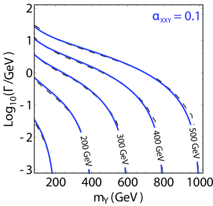
Figure 3: Relation of the $s$-channel width $\Gamma_{Y}$ and mass $m_{Y}$ for a pole below threshold consistent with cosmological relic density $\Omega h^{2}=0.1$. Dashed curves (black online) are the numerical calculation. Solid curves (blue online) are the analytic relation of Eq. 6. Each curve is evaluated with a fixed dark matter mass $m_{X}$ =100-500 GeV in 100 GeV increments.

II.1 Analytic Representation

Observe in Fig. 3 that each dashed (black) curve moving to the right terminates in a region of $\Gamma_{Y}\rightarrow 0$. Near the threshold everything is determined by the degree of the zero of the function, $\Gamma_{Y}\sim(m_{Y}-2m_{X})^{n}$. The power $n=2$ can be gotten analytically, but was also fit directly with numerical work. Then we know $\Gamma_{Y}\sim(1-m_{Y}/2m_{X})^{2}$, times a known factor of $m_{X}$

In the opposite extreme of $m_{Y}<<2m_{X}$ the velocity averaged cross section ${\langle\sigma v\rangle}$ reduces to another simple analytic result:

$${\langle\sigma v\rangle}(m_{Y}<<2m_{X})\rightarrow\frac{\pi\alpha_{XXY}C_{jj^{\prime}}}{4m_{X}^{4}}m_{Y}\Gamma_{Y}$$ (4)

Notice the dependence going like $1/(m_{Y}\Gamma_{Y})$. Inverting the equation gives

$$\Gamma_{Y}\rightarrow{4m_{X}^{4}\over\pi\alpha_{XXY}C_{jj^{\prime}}m_{Y}}{\langle\sigma v\rangle}$$ (5)

The limit of small connector mass $m_{Y}\rightarrow 0$ with $\Gamma_{Y}<<2m_{X}$ approaches the Born approximation, and for us is the unique case where the Born cross section is relevant. In the Born limit we know ${\langle\sigma v\rangle}\rightarrow 3\times 10^{-26}cm^{3}/s$, which fixes one overall scale. Then accounting for factors of $m_{X}$ gives

$$\Gamma_{Y}\sim{4m_{X}^{3}\over\pi C_{jj^{\prime}}\alpha_{XXY}}(2.6\times 10^{-9}GeV^{-2})$$

$$\times\left(1-\frac{m_{Y}}{2m_{X}}\right)^{2}{m_{X}\over m_{Y}}g(m_{Y}/m_{X}).$$

The dimensionless interpolating function $g(m_{Y}/m_{X})$ remains. It must obey $g\rightarrow 1$ when $m_{Y}<<2m_{X}$, suggesting a polynomial expansion $g\sim 1+\sum_{k}\,g_{k}(m_{Y}/m_{X})^{k}$. Two terms suffice with $g_{1}=2$. Our analytic formula for the pole below threshold mass-width relation is then

$$\Gamma_{Y} = {8\over\pi}{1\,GeV\over C_{jj^{\prime}}\alpha_{XXY}}\left({m_{X}\over 730\,GeV}\right)^{3}$$ (6)

$$\times \left(1+{m_{X}\over 2m_{Y}}\right)\left(1-\frac{m_{Y}}{2m_{X}}\right)^{2},$$

$$\>\>\>\>\>for\>m_{Y}<2m_{X}$$

The fit of the formula to the numerical work is extremely good. Fig. 3 shows a typical example.

We have already noted that Eq. 6 generalizes and replaces the traditional formula ${\langle\sigma v\rangle}=3\times 10^{-26}cm^{3}/s$. The formula accounts for the fact that intermediate states of all particles coupling to dark matter are either absolutely stable or have a finite lifetime. To underscore the difference, compare the traditional counting rules, motivated on dimensional analysis, using annihilation cross sections of order 1-picobarn. Under the assumption $\sigma v\sim\alpha_{X}^{2}/m_{X}^{2}\sim pb$, a typical upper limit $\alpha_{X}^{2}\lesssim 10^{-4}$ would imply $m_{X}\lesssim 200$ GeV. This well-known result needs a finely tuned mass-couping relation to make a Universe. Our formula contains far more information, and reveals the hidden assumption that $m_{Y}<<m_{X}$ was implicitly assumed for the traditional formula to be consistent.

II.2 Replacement Rule for Adding Non-Resonant Channels

Some models of dark matter annihilation include more than one channel. No matter how many channels are involved, as long as the $s$-channel is a part of the model, the mass-width relation of Eq. 6 can be generalized.

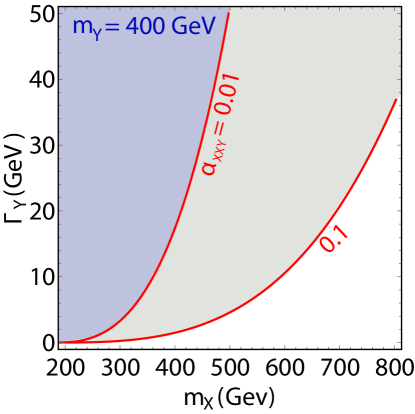
Figure 4: Upper limits on $\Gamma_{Y}$ assuming $s$-channel annihilation (pole below threshold) plus other channels increasing the cross section. Shaded regions to the left and above the contours are not allowed. Curves show different couplings $\alpha_{XXY}=g_{XXY}^{2}/4\pi$; $m_{Y}=400$ GeV is used for the purpose of the graphic. Larger $m_{Y}$ pushes contours to the right.

For definiteness, suppose the addition of other processes increases the annihilation rate. Then the theory keeping $\Omega h^{2}$ fixed will require smaller $\Gamma_{Y}$, all other things fixed. That condition rules out all contours to the right and above the contours shown in Fig. 3 created by $s$-channel dominance. The allowed region to the right and below each line implies an inequality (Fig. 4) :

$$\Gamma_{Y} \leq {8\over\pi}\left({1\,GeV\over C_{jj^{\prime}}\alpha_{XXY}}\right)\left({m_{X}\over 730\,GeV}\right)^{3}$$ (7)

$$\times\left(1+{m_{X}\over 2m_{Y}}\right)\left(1-\frac{m_{Y}}{2m_{X}}\right)^{2}.$$

While cross sections often increase when channels are added, destructive interference occurs in some models. In that case the inequality reverses the sign.

To illustrate the use of Eq. 7, suppose a new vector boson ($Z^{\prime}$ perhaps) is discovered at the LHC. Measuring the resonance observed in any channel will give its mass $m_{Y}$, and the total width $\Gamma_{Y}$. Applying Eq. 7 then gives the consistent $m_{X},\,\alpha_{XXY}$ parameter space regions consistent with relic abundance without a need for an extensive numerical parameter space scan. These predicted coupling relations are then compared to the information from production rate and branching ratio into particular channels seen in the experiment.

A new relation comes from a “replacement rule.” Let the total velocity averaged cross section be expressed as

$${\langle\sigma v\rangle}_{tot}={\langle\sigma v\rangle}_{s}+{\langle\sigma v\rangle}_{other}.$$

Suppose ${\langle\sigma v\rangle}_{other}$ happens to be consistent with the traditional Born-style of approximation, by which

$${\langle\sigma v\rangle}_{other}=\sum_{i}\alpha^{i}_{eff}/m_{X}^{2},$$

where $\alpha^{i}_{eff}$ is an effective coupling to the $i^{th}$ channel. (An example model in the context of heavy hidden sector dark matter can be found in Ref. MarchRussell:2008yu .) Matching the extreme limits produces the replacement rule. If the $s$-channel pole is near the threshold, the mass width relation should approach Eq. 6. If the pole is far from threshold the resonant cross section approaches an effective Born-level cross section, and adds to it. That implies a boundary condition of ${\langle\sigma v\rangle}_{s}+{\langle\sigma v\rangle}_{other}\approx 10^{-9}GeV^{-2}$ at this endpoint. Reviewing how that scale previously entered the analysis suggests a replacement rule:

$$2.6\times 10^{-9}GeV^{-2}\rightarrow 2.6\times 10^{-9}{GeV}^{-2}-{\sum_{i}\alpha^{i}_{eff}\over m_{X}^{2}}$$ (8)

The revised mass-v-width relation then becomes

$$\Gamma(m_{Y}) = {8\over\pi}{1\,GeV\over C_{jj^{\prime}}\alpha_{XXY}}\left[1-\sum_{i}\alpha^{i}_{eff}\left({730\,GeV\over m_{X}}\right)^{2}\right]$$

$$\times\,\,({m_{X}\over 730\,GeV})^{3}\left(1+\frac{m_{X}}{2m_{Y}}\right)\left(1-\frac{m_{Y}}{2m_{X}}\right)^{2}$$

Fig. 5 shows the replacement rule performs quite well. Not surprisingly, the difference relative to a pure $s$-channel annihilation model increases for smaller $m_{X}$. This is because the individual cross section contributions from other channels shown in Eq. LABEL:newanappx scale uniformly like $1/m_{X}^{2}$.

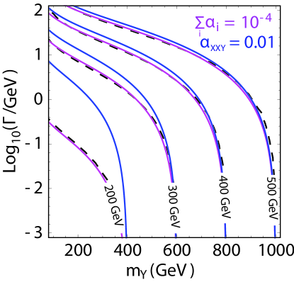
Figure 5: Generalization of the mass-width relation to include “Born-like” channels. Black dashed curves show numerical evaluation. Solid curves (magenta online) are the revised fit of Eq. LABEL:newanappx. Thick solid curves (blue online) are the approximations of Eq. 6, consistent with the role as an upper bound. Different curves use different masses $m_{X}=100-500GeV$, from left to right. Parameter $\alpha_{XXY}=10^{-2}$ and $\sum_{i}\alpha_{eff}^{i}=10^{-4}$ for the purpose of the graphic.

III Calculable Widths Constrain the Masses

Up to here we have considered the width $\Gamma_{Y}$ as an independent parameter. In this section we go a step further and consider widths as quantities which can be calculated. When we say that “widths are calculable” it emphasizes the facts that (1) most theories are perturbatively coupled, and (2) most of the width will usually occur in a finite number of channels. Whatever the model, combining the calculation of the width with the mass-width relation creates a new relation.

The differential rate $d\Gamma$ of a general decay of a particle of mass $m_{Y}$ is given by

$$d\Gamma\sim{1\over 2m_{Y}}|M|^{2}dLIPS.$$

Symbol $M$ is the amplitude. The final state phase space of two identical particles yield $\int dLIPS_{2}\sim v_{f}$ where $v_{f}$ is the velocity of either final state particle in the center of mass frame. In many cases the width is dominated by relativistic final states, $v_{f}\rightarrow 1$. It would be unusual, and a case of rather fine tuning, for all channels with phase space limitations $v_{f}<<1$ to dominate the total width. Barring that event, by dimensional analysis, the width of a heavy particle with dimensionless coupling generally goes like its mass:

$$\Gamma_{Y}\sim\alpha_{\Gamma}m_{Y}.$$ (10)

We make this an equality allowing symbol $\alpha_{\Gamma}$ to absorb coupling constants, the number of important channels, and model details. The general scaling of widths-proportional-to-mass is rather kinematic. However, if a dimensionful coupling is introduced, then the mass dependence of rest of the calculation is dominated by dimensional analysis again. Keeping in mind that $\alpha_{\Gamma}$ stands for the width actually calculated in a particular model, we continue.

With $\alpha_{\Gamma}$ fixed, the formula for $\Gamma_{Y}$ is an increasing function of $m_{Y}$. Meanwhile the $s$-channel mass-v-width requirements are all decreasing functions of $m_{Y}$ (Fig. 3, Eq. 6, Eq. LABEL:newanappx). Then the width-v-mass relation always matches the $s$-channel mass-v-width relation at a definite point. Fig. 6 shows $\Gamma_{Y}=\alpha_{\Gamma}m_{Y}$ as red curves, whose intersections with the blue curves constrain the masses.

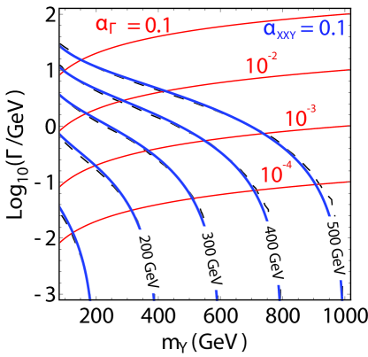
Figure 6: Combining the below-threshold width-v-mass $m_{Y}$ relation of Fig. 3 with $\Gamma_{Y}=\alpha_{\Gamma}m_{Y}$ represented by solid thin curves (red online). Intersections of the curves predict a non-linear relation between $m_{X}$ and $m_{Y}$ (text). Values of $\alpha_{\Gamma}=10^{-1}$ (top curve) range to $\alpha_{\Gamma}=10^{-4}$ (bottom curve) in factor of 10 increments.

Inspection finds a surprising fact. Rather weakly coupled theories ($\alpha_{\Gamma}\lesssim 10^{-4}$) only intersect the relic curves in the region where $m_{Y}\approx 2m_{X}$. In minimal supersymmetry, this result corresponds to the so called higgs ”funnel” region of $m_{0},m_{1/2}$ parameter space. However, our result is much more general and extends beyond the assumptions of SUSY.

The two couplings, $\alpha_{\Gamma}$ and $\alpha_{XXY}$ act in the same direction. Smaller $\alpha_{\Gamma}$ makes smaller widths that force the system into the threshold region to be viable. Smaller $\alpha_{XYY}$ worsens the situation by pushing the contours of constant $\Omega h^{2}$ up in the $\Gamma_{Y}-m_{Y}$ plane. The trend of both pushes masses into very near coincidence of $m_{Y}\sim 2m_{X}$, which we call a “finely-tuned threshold.”

Except for bound state formation we have no reason to consider finely-tuned thresholds very plausible, but we can afford to stay neutral. Bound states have been discussed in detail in Refs. Shepherd:2009sa ; MarchRussell:2008tu . Some basic relations between bound state widths and masses are reviewed in Ref. Backovic:2009rw . Bound state relations are very specific and require separate treatment that is not our topic here.

Our mass-width relation allows for classification of models according to the degree of fine tuning. For example, Fig. 6 shows a theory with $\alpha_{XXY}=0.1$. The intersections are not very demanding, and the theory is not finely tuned for $\alpha_{\Gamma}\geq 10^{-3}$. However the same theory using $\alpha_{XXY}=10^{-3}$ will require widths $100$ times bigger for the same $m_{Y}$ to keep $\Omega h^{2}$ constant. At that point all contours are pushed up to such a degree we’d find the theory finely-tuned for all reasonable $\Gamma_{Y}$.

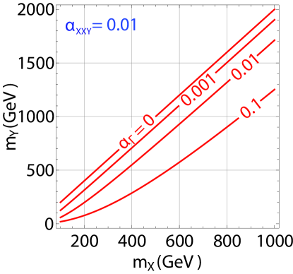
Figure 7: Mass of dark matter $m_{X}$ versus the mass of the particle in the $s$-channel $m_{Y}$. Red lines represent $\alpha_{\Gamma}=0.001,0.01,0.1$ from top to bottom. $\alpha_{XXY}=0.01$ for the purpose of the graphic. Small widths ($\alpha_{\Gamma}$ small) require fine mass tuning, $m_{Y}\approx 2m_{X}$ to accommodate correct relic abundance.

III.1 Dark Matter and Pole Mass Relations

So far we have looked at an $m_{Y}$ - $\Gamma_{Y}$ relationship, given $m_{X}$. It is very interesting to consider the relation between $m_{Y}$ and $m_{X}$ given $\alpha_{\Gamma}$. Fig. 7 shows the mass relationships for different values of $\alpha_{\Gamma}$. Once again $\alpha_{\Gamma}\rightarrow 0$ forces the resonance into the finely tuned region of $m_{Y}\approx 2m_{X}$.

Solving Eq. 6 yields a cubic equation fixing $m_{Y}=m_{Y}(m_{X},\alpha_{XXY},\alpha_{\Gamma})$. The relationship is nearly linear for a wide range of $m_{X}$. Collect the couplings into a new symbol

$$\alpha_{\kappa}^{2}={\alpha_{XXY}\alpha_{\Gamma}C_{jj^{\prime}}\over 10^{-4}}$$

Note the symbol has been re-scaled in units of $\alpha_{XXY}/10^{-2}$, $\alpha_{\Gamma}/10^{-2}$ we find reasonable. The series expansion for large $m_{X}$ is found to be

$$m_{Y}\approx 2m_{X}-313GeV\alpha_{\kappa}+40.2GeV\,\alpha_{\kappa}^{2}\,({730GeV\over m_{X}})$$

$$-5.87GeV\,\alpha_{\kappa}^{3}\,({730GeV\over m_{X}})^{2}+...$$ (11)

Eq. 11 with only the first two terms kept is essentially exact for $\alpha_{\kappa}\lesssim 1,\,m_{X}\gtrsim 100$ GeV, while for $\alpha_{\kappa}\gtrsim 1$ a numerical evaluation is preferable.

Analyzing Fig. 7 and 8 we notice that the mass range of 100-500 GeV does not require extreme fine tuning for a reasonable range of perturbative couplings. On the other hand the regime of $m_{X}>>100GeV$ seems to require a pole tuned very finely according to Eq. 11.

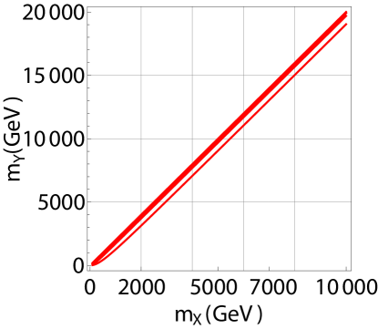
Figure 8: Same as Fig. 7 but for an extended range of $m_{X}$. Red lines represent $\alpha_{\Gamma}=0.001,0.01,0.1$ from top to bottom. $\alpha_{XXY}=0.01$ for the purpose of the graphic.

IV Mass-Width Relations: Pole Above Threshold ($m_{Y}>2m_{X}$)

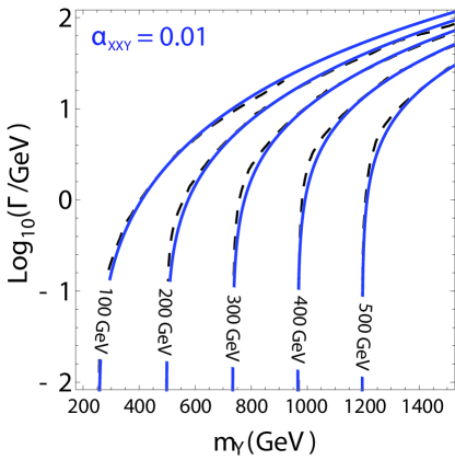
Figure 9: Relation of the $s$-channel width $\Gamma_{Y}$ and pole mass $m_{Y}$ above threshold consistent with cosmological relic density $\Omega h^{2}=0.1$. Dashed curves (black online) are the numerical calculation. Solid curves (blue online) are the analytic relation of Eq. 16. Each curve is evaluated with a fixed dark matter mass $m_{X}$ =100-500 GeV in 100 GeV increments.

The relic abundance calculation for a pole above threshold is complicated by a saddle point in the integration of ${\langle\sigma v\rangle}$. To begin we again consider the extreme limits. For $m_{Y}>>2m_{X}$ the velocity averaged cross section reduces to

$${\langle\sigma v\rangle}(m_{Y}>>2m_{X})\rightarrow{4\pi\alpha_{XXY}C_{jj^{\prime}}\over m_{Y}^{3}}\Gamma_{Y}.$$ (12)

By construction this limit reproduces the Born-level estimate, ${\langle\sigma v\rangle}\approx 10^{-9}GeV^{-2}$. Introduce a dimensionless function $h$ to describe other limits, expressed by

$$\Gamma_{Y} \sim {m_{Y}^{3}\over 4\pi\alpha_{XXY}C_{jj^{\prime}}}(6.4\times 10^{-9}GeV^{-2})$$

$$\times h(m_{Y},\,m_{X},\,A,\,\alpha_{XXY}C_{jj^{\prime}}).$$

We have normalized $h\rightarrow 1$ for $m_{Y}>>2m_{X}$ by absorbing the overall normalization into $6.4\times 10^{-}9GeV^{-2}$, suggesting the ansatz

$$h=1-{\eta\,m_{X}\over m_{Y}},$$ (13)

where $\eta$ is the measure of the ”offset” of $m_{Y}$ from the threshold $2m_{X}$. Unlike the case of pole below threshold, the saddle point causes $\eta$ to be a function of $m_{X}$ and a relic scale parameter, which we call $A$.

Figure 10: Mass of dark matter $m_{X}$ vs. the mass of the $s$-channel particle $m_{Y}$ for a pole above threshold, $m_{Y}>2m_{X}$ Red lines represent $\alpha_{\Gamma}=0,0.01,0.05,0.1$ from top to bottom. $\alpha_{XXY}=0.01$ for the purpose of the graphic. Small widths ($\alpha_{\Gamma}$ small) require very fine tuning of masses, $m_{Y}\approx\eta m_{X}$ to accommodate correct relic abundance.

The extreme of $\Gamma\rightarrow 0$ gives more information about the function $h$. The Breit-Wigner factor can be approximated as

$${\Gamma m_{Y}\over(s-m_{Y}^{2})^{2}+(m_{Y}\Gamma)^{2}}\rightarrow\pi\delta(s-m_{Y}^{2}).$$ (14)

The Boltzmann equation is then solved analytically in terms of error functions, predicting $h$ and $\eta$ in this limit:

$$\eta(m_{X},\alpha_{XXY},C_{jj^{\prime}})\equiv 2\sqrt{1+{2\,\over x_{d}}erfc^{-1}({A\,m_{X}^{2}\over\alpha_{XXY}C_{jj^{\prime}}})},$$ (15)

where $A=1.3\times 10^{-11}GeV^{-2}$ gives a good fit for all reasonable $m_{Y}$ and $\Gamma_{Y}$. The lower integration limit $x_{d}$ is computed in a self consistent way and we find that the standard value of $x_{d}=30$ is appropriate.

Eq. 15 involves the inverse complementary error functions ($erfc^{-1}$), which is somewhat cumbersome. While many numerical packages (including Mathematica) compute it, a simpler analytic formulation of $\eta$ is useful. Let $z=A\,m_{X}^{2}/\alpha_{XXY}C_{jj^{\prime}}$. We find the approximation

$$\eta(z)\approx 1.978-0.521z-0.051Log[z]$$

is almost exact in the range $10^{-8}\leq z\leq 1$.

Our analytic formula for a pole above threshold is now:

$$\Gamma_{Y} = {1GeV\over 4\pi\alpha_{XXY}C_{jj^{\prime}}}\left({m_{Y}\over 589GeV}\right)^{3}\left(1-{\eta(z)\,m_{X}\over m_{Y}}\right),$$ (16)

$$\>\>\>\>\>for\>m_{Y}>2m_{X}$$

Once again, the analytic approximation matches numerical work remarkably well. Fig. 9 shows an example.

Eq. 16 reveals more finely tuned parameter regions for a pole above threshold. In the limit $\Gamma_{Y}\rightarrow 0$, $m_{Y}$ is finely tuned to $\eta m_{X}$, as seen in Fig. 10. The competition between the pole position, width, and thermal Gaussian are all summarized by this generalization of the pole below-threshold relation.

As before, eliminating $\Gamma_{Y}=\alpha_{\Gamma}m_{Y}$ produces an $m_{X}-m_{Y}$ relation:

$$m_{Y}={\eta(z)m_{X}\over 2}+{1\over 2}\sqrt{\eta^{2}(z)m_{X}^{2}+16\pi\mu^{2}\alpha_{\Gamma}\alpha_{XXY}C_{jj^{\prime}}},$$

where $\mu^{2}=589^{3}GeV^{2}$.

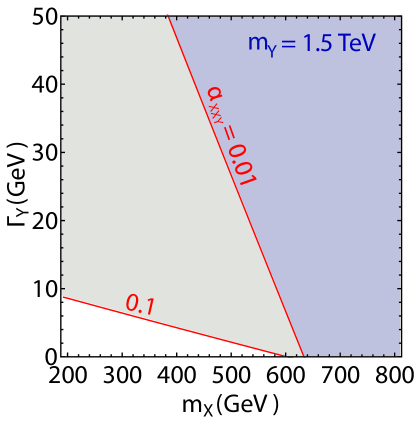
Figure 11: Typical upper limits on $\Gamma_{Y}$ given a mass $m_{Y}$ for different masses of dark matter $m_{X}$ assuming both $s$-channel annihilation (pole above threshold) and other non-resonant channels. Shaded regions to the left and above the contours are not allowed. $m_{Y}=1.5$ TeV was used for the purpose of the graphic; larger $m_{Y}$ pushes contours to the right.

IV.0.1 Upper Limit on $m_{X}$

The particular form of the ”offset function” $\eta$ yields an upper limit on $m_{X}$. From the derivation the argument of $erfc^{-1}$ must be less than one, which implies

$$m_{X}\leq 2.77\times 10^{5}GeV\sqrt{\alpha_{XXY}C_{jj^{\prime}}}$$ (17)

This formula is more precise than supposing $m_{Y}$ is bounded by a Born-level estimate and $2m_{X}<m_{Y}$. Consider for example a small coupling $\alpha_{XXY}=10^{-4}$. Consistency with relic abundance requires dark matter masses $m_{X}\lesssim 2.8TeV$.

IV.0.2 Inequalities for Non-Resonant Channels

Generalization of the above-threshold mass width relation to allow for non-resonant channels is similar to the below-threshold case. When ${\langle\sigma v\rangle}_{tot}\geq{\langle\sigma v\rangle}_{s}$ the mass width relation becomes

$$\Gamma_{Y}\leq{1GeV\over 4\pi\alpha_{XXY}C_{jj^{\prime}}}\left({m_{Y}\over 589GeV}\right)^{3}\left(1-{\eta\,m_{X}\over m_{Y}}\right).$$ (18)

An illustration of the inequality can be seen in Fig. 11. Notice that for large couplings, i.e. $\alpha_{XXY}>0.1$ major portions of the parameter space can be ruled out. The termination point ($\Gamma_{Y}\rightarrow 0$) is simply the $\eta m_{X}=m_{Y}$ point, giving us another bound on $m_{X}$. By inspection, a coupling $\alpha_{XXY}=0.1$ and $m_{Y}=1.5TeV$ requires $m_{X}\lesssim 600GeV$.

V Conclusions

The dynamical effects of resonant processes and finite particle widths play an important role in dark matter evolution in the early universe. The Born approximation is seldom adequate because the non-relativistic velocity dependence of cross sections drives decoupling. Organizing the calculation in terms of observable quantities gives new relations between the masses and widths of intermediate states that will be consistent with fixed relic abundance.

Given that particle widths are generally calculable, our mass-v-width relations develop into mass-v-mass consistency relations between the dark matter with a given relic density and the mass of an $s$-channel connector. Depending on the model, this produces a significant revision of a traditional rule ${\langle\sigma v\rangle}\sim 3\times 10^{-26}\,cm^{3}/s$. The relation between $m_{X}$ and $m_{Y}$ depends on the way the width is calculated, but in a broad class of models permits an unlimited range of both masses. Our relations can be used to test candidates for dark matter in LHC-based experiments, while also eliminating much of the need to re-compute relic evolution on a model-by-model basis.

Acknowledgments: We thank Yudi Santoso and KC Kong for helpful discussions. Research supported in part under DOE Grant Number DE-FG02-04ER14308.

References

- (1) K. Griest and D. Seckel, Phys. Rev. D bf43, 3191 (1991).
- (2) M. Ibe, Y. Nakayama, H. Murayama and T. T. Yanagida, JHEP bf0904, 087 (2009) [arXiv:0902.2914 [hep-ph]].
- (3) K. Kadota, K. Freese and P. Gondolo, arXiv:1003.4442 [hep-ph].
- (4) K. Cheung and T. C. Yuan, JHEP bf0703, 120 (2007) [arXiv:hep-ph/0701107].
- (5) J. Kumar and J. D. Wells, Phys. Rev. D bf74, 115017 (2006) [arXiv:hep-ph/0606183].
- (6) T. Han, Z. Si, K. M. Zurek and M. J. Strassler, JHEP bf0807, 008 (2008) [arXiv:0712.2041 [hep-ph]].
- (7) M. Backovic and J. P. Ralston, Phys. Rev. D bf81, 056002 (2010) [arXiv:0910.1113 [hep-ph]].
- (8) O. Adriani et al. [PAMELA Collaboration], Nature bf458, 607 (2009) [arXiv:0810.4995 [astro-ph]].
- (9) E. A. Baltz et al., JCAP bf0807, 013 (2008) [arXiv:0806.2911 [astro-ph]].
- (10) S. Torii et al. [PPB-BETS Collaboration], arXiv:0809.0760 [astro-ph].
- (11) S. W. Barwick et. al. , [HEAT Collaboration] Astrophys.J. 482 (1997) L191-L194
- (12) J. Chang et. al. , Nature 456. (2008)
- (13) J. Zavala, M. Vogelsberger and S. D. M. White, Phys. Rev. D bf81, 083502 (2010) [arXiv:0910.5221 [astro-ph.CO]].
- (14) J. L. Feng, M. Kaplinghat and H. B. Yu, arXiv:1005.4678 [hep-ph].
- (15) J. B. Dent, S. Dutta and R. J. Scherrer, Phys. Lett. B bf687, 275 (2010) [arXiv:0909.4128 [astro-ph.CO]].
- (16) M. Ibe, H. Murayama and T. T. Yanagida, Phys. Rev. D bf79, 095009 (2009) [arXiv:0812.0072 [hep-ph]].
- (17) W. L. Guo and Y. L. Wu, Phys. Rev. D bf79, 055012 (2009) [arXiv:0901.1450 [hep-ph]].
- (18) N. Baro, F. Boudjema and A. Semenov, Phys. Lett. B bf660, 550 (2008) [arXiv:0710.1821 [hep-ph]].
- (19) M. Drees, J. M. Kim and K. I. Nagao, Phys. Rev. D bf81, 105004 (2010) [arXiv:0911.3795 [hep-ph]].
- (20) S. Bhattacharya, U. Chattopadhyay, D. Choudhury, D. Das and B. Mukhopadhyaya, Phys. Rev. D bf81, 075009 (2010) [arXiv:0907.3428 [hep-ph]].
- (21) A. Djouadi, M. Drees and J. L. Kneur, Phys. Lett. B bf624, 60 (2005) [arXiv:hep-ph/0504090].
- (22) J. R. Ellis, S. F. King and J. P. Roberts, JHEP bf0804, 099 (2008) [arXiv:0711.2741 [hep-ph]].
- (23) A. B. Lahanas and V. C. Spanos, Eur. Phys. J. C bf23, 185 (2002) [arXiv:hep-ph/0106345].
- (24) B. Herrmann and M. Klasen, Phys. Rev. D bf76, 117704 (2007) [arXiv:0709.0043 [hep-ph]].
- (25) S. Y. Choi and Y. G. Kim, Phys. Lett. B bf637, 27 (2006) [arXiv:hep-ph/0602109].
- (26) G. Belanger, F. Boudjema, S. Kraml, A. Pukhov and A. Semenov, Phys. Rev. D bf73 (2006) 115007 [arXiv:hep-ph/0604150].
- (27) E. W. Kolb,M. S. Turner, The Early Universe, Addison-Wesley, MA, (1990)
- (28) J. March-Russell, S. M. West, D. Cumberbatch and D. Hooper, JHEP bf0807, 058 (2008) [arXiv:0801.3440 [hep-ph]].
- (29) W. Shepherd, T. M. P. Tait and G. Zaharijas, Phys. Rev. D bf79, 055022 (2009) [arXiv:0901.2125 [hep-ph]].
- (30) J. D. March-Russell and S. M. West, Phys. Lett. B bf676, 133 (2009) [arXiv:0812.0559 [astro-ph]].