Dispersion and damping of two-dimensional dust acoustic waves: Theory and Simulation

Abstract

A two-dimensional generalized hydrodynamics (GH) model is developed to study the full spectrum of both longitudinal and transverse dust acoustic waves (DAW) in strongly coupled complex (dusty) plasmas, with memory-function-formalism being implemented to enforce high-frequency sum rules. Results are compared with earlier theories (such as quasi-localized charge approximation and its extended version) and with a self-consistent Brownian dynamics simulation. It is found that the GH approach provides good account, not only for dispersion relations, but also for damping rates of the DAW modes in a wide range of coupling strengths, an issue hitherto not fully addressed for dusty plasmas.

1 Introduction

Dusty, or complex plasmas have grown into a mature research field with a surprisingly broad range of interdisciplinary facets [1, 2, 3]. There has been significant interest in the study of dynamics of collective excitations of dusty plasmas, both in experiments [4, 5, 6, 7, 8, 9, 10] and through theory/numerical simulation of strongly-coupled Yukawa systems [11, 12, 13, 14, 15, 16, 17, 18, 19, 20, 21, 22, 23]. Of particular interest in these studies is theoretical modeling of longitudinal and transverse dust acoustic wave (DAW) modes [11], and consequently several assessments of how the existing analytical theories compare with the results from computer experiments have appeared recently [19, 20, 22, 23, 24]. Specifically, by comparing the Brownian dynamics (BD) simulation results for the DAW spectra with various theoretical models, it was shown that the so-called Quasi-localized charge approximation (QLCA) [15, 20] provides an overall good account of the DAW dispersion relations, i.e., the peak locations in those spectra, for both three-dimensional (3D) and two-dimensional (2D) dusty plasma states characterized by the coupling strength $\Gamma$ in the range $10<\Gamma<1000$ [22, 24]. However, since the QLCA provides no information about the profile of such spectra and, consequently, gives no account of damping processes for the collective modes [15], it is desirable to explore alternate theoretical approaches to strongly coupled systems. In that context, generalized hydrodynamics (GH) offers possibility to describe full wave spectra by introducing viscoelastic effects in the dynamics of dusty plasmas in a phenomenological manner, as was demonstrated in studying DAWs in 3D dusty plasmas [12, 13, 14].

In contrast to ordinary hydrodynamics (OH), which is only valid for weakly coupled fluids with $\Gamma\ll 1$ in the long wavelength limit, GH covers wider ranges of coupling strengths and wavelengths, where structural effects begin to show up. Particularly suitable and physically intuitive framework for implementing the GH model is provided by descriptions of the Lennard-Jones fluids, pioneered by Ailawadi et al. [25], Boon and Yip [26], and Hansen and McDonald [27]. This framework may be applied to a dusty plasma by asserting that dust particles form a quasi-neutral fluid with the inter-particle interactions described via a Debye-Hückel, or Yukawa potential, which arises due to screening of the charge accumulated on dust particles by the background electron and ion fluids. Successful applications of the GH model to dusty plasma were conducted by Kaw and Sen [13] and Murillo [14] to study the wave dispersion and the shear wave cutoff in 3D dust liquids, respectively.

However, there is still great demand for a GH model for 2D strongly coupled dusty plasmas (SCDPs), especially because such systems have become particularly favored in recent laboratory experiments [3, 28]. Therefore, our principal motivation in this work is to develop and implement a GH model for studying the collective dynamics in 2D SCDPs. In addition, it is necessary to generalize the GH model to include the effects of collisions of dust particles with the neutral gas in the background plasma in a manner similar to that used for colloidal suspensions in describing the collisions of macroions with the solvent molecules [29]. While such collisions give rise to the classical Brownian motion of macroparticles in both these systems, it should be stressed that the friction forces on dust particles due to the neutrals in dusty plasmas are generally much weaker than the friction forces on the colloidal macroions. Accordingly, effects of the neutral gas on the DAW dispersion relations are found to be negligible for the range of parameters of interest in experiments with dusty plasmas, thus validating the use of molecular dynamics (MD) simulations for such systems [24]. However, it is still unclear as to what extent can damping due to the neutral gas compete with the viscous damping of longitudinal DAWs at finite frequencies and finite wavelengths in dusty plasmas [30]. While this difficult issue naturally arises in this work, our primary motivation in using BD simulation lies in the fact that treating the dust particles as Brownian particles provides a natural and convenient way to eliminate the need for thermostation that arises in the MD simulation of dusty plasmas [22, 31].

In this paper we perform a BD simulation of strongly coupled 2D Yukawa liquids, and use the results to evaluate the equilibrium radial distribution function (RDF) and the static structure factor, as well as the (power) spectral densities for both the longitudinal and transverse current densities in such systems. The former two quantities enable us to use the GH approach within the memory function formalism to evaluate both the dispersion relation and the damping rate of the DAW modes in 2D dusty plasmas by enforcing the low-order, high-frequency sum rules upon the theoretical spectral densities. It is found that the GH approach provides dispersion relations that compare well with those resulting from the simulation spectra over broad ranges of wavelengths and coupling strengths. Additional comparison with the dispersion relations from the QLCA model shows that the GH approach provides a good account of the direct thermal effect at lower coupling strengths and shorter wavelengths, which is absent in the QLCA approach, but is seen in the simulation data. On the other hand, a simple extension of the QLCA dispersion relation, which was recently proposed in Ref. [22], is found to be in a much better agreement with both the GH results and simulation data. Most importantly, the GH results are shown to yield a good fit to the spectral density profiles from our BD simulations, thus providing semi-analytical modeling of the wave-number dependent damping rates of the DAW modes in strongly coupled dusty plasmas in a broad range of coupling strengths, an issue that has not been fully addressed so far [22]. Finally, we also find that the effect of collisions with the neutrals on the DAW damping rates is well accounted for by introducing a local in time friction force into the GH equations.

The manuscript is organized as follows. The details of the BD simulation are given in Section 2. Theoretical development of the generalized hydrodynamics is discussed in Section 3. Results based on two simple models for the memory function are presented in Section 4, while we conclude in Section 5.

2 Simulation

We perform BD simulation of a 2D system consisting of $N=4000$ dust particles, each carrying a constant charge $q_{d}$, which are initially placed at random positions within a square simulation cell in the $\mathbf{r}=(x,y)$ plane with periodic boundary conditions. Evolution of the system is governed by equations that may be regarded as a stochastic generalization of the usual MD method, where the effect of collisions with the neutral particles in the background plasma is modeled by a Langevin generalization of the usual Newton’s equations. Therefore, equations for the velocity and the position vectors of the $i$-th dust particle are given by

$$\frac{d\mathbf{v}_{i}(t)}{dt} = -\gamma_{n}\mathbf{v}_{i}(t)+\frac{1}{m_{d}}\sum_{j\neq i}\mathbf{F}\!\left(\mathbf{r}_{i}(t)\!-\!\mathbf{r}_{j}(t)\right)+\mathbf{A}_{i}(t),$$

$$\frac{d\mathbf{r}_{i}(t)}{dt} = \mathbf{v}_{i}(t),$$ (1)

where $m_{d}$ is the mass of each dust particle and $\mathbf{F}(\mathbf{r})=-(\mathbf{r}/r)dU(r)/dr$ is the pair-wise force between two dust particles a distance $r=\sqrt{x^{2}+y^{2}}$ apart, interacting via the Yukawa potential, $U(r)=(q_{d}^{2}/r)\exp\left(-r/\lambda_{D}\right)$, with $\lambda_{D}$ being the Debye screening length of electrons and ions in the background plasma. Collisions of the $i$-th dust particle with the neutrals in the plasma give rise to a systematic drag force, which we model by the Epstein drag coefficient $\gamma_{n}$, and to a cumulative random force, which we model by a delta-correlated Gaussian white noise. When the system is in thermal equilibrium, the friction coefficient $\gamma_{n}$ and the stochastic acceleration of the $i$-th particle $\mathbf{A}_{i}(t)$ are related to the ambient temperature $T_{d}$ via the fluctuation-dissipation theorem. Equations (1) are solved for our system by the Gear-like predictor-corrector algorithm for BD simulation [31], which was previously used in modeling both the equilibrium structure [32] and collective modes in 2D dusty plasmas [22].

Equations (1) can be expressed in terms of just three parameters [22]: the coupling strength $\Gamma=q_{d}^{2}/\left(ak_{B}T_{d}\right)$, the reduced neutral drag coefficient $\gamma=\gamma_{n}/\omega_{pd}$, and the screening parameter $\kappa=a/\lambda_{D}$, where $a\equiv 1/\sqrt{\pi\rho}$ is the average inter-particle separation with $\rho$ being the average surface density of dust particles, and $\omega_{pd}=\sqrt{2q_{d}^{2}/\left(m_{d}a^{3}\right)}$ is the characteristic dust-plasma frequency. In this work, we perform BD simulations using $\gamma=0.06$ (which is a value chosen as a matter of convenience only) and $\kappa$ = 1 as standard values, in a range of coupling strengths $20\leq\Gamma\leq 1000$ covering liquid-to-crystalline states of dusty plasma [22].

Further, the current density of dust particles is defined as

$$\mathbf{j}(\mathbf{r},t)=\frac{1}{\sqrt{N}}\sum^{N}_{i=1}\mathbf{v}_{i}(t)\delta(\mathbf{r}-\mathbf{r}_{i}(t)),$$ (2)

with the Fourier transform of its cartesian component $\alpha$ given by

$$j_{\alpha}(\mathbf{k},t)=\frac{1}{\sqrt{N}}\sum^{N}_{i=1}v_{i\alpha}(t)e^{i\mathbf{k}\cdot\mathbf{r}_{i}(t)}.$$ (3)

Assuming that the dust collective modes propagate along the $x$-direction, i.e., $\mathbf{k}=(k,0)$, we let $\alpha=x$ or $y$, allowing us to define the corresponding longitudinal or transverse current density auto-correlation functions as

$$C_{l,t}(k,t)=\langle j^{*}_{l,t}(\mathbf{k},0)j_{l,t}(\mathbf{k},t)\rangle,$$ (4)

where the angular brackets denote ensemble averaging over the initial time. The longitudinal/transverse spectral densities are then obtained as the Fourier transform of the respective current density auto-correlation functions as,

$$P_{l,t}(k,\omega)=\int^{\infty}_{-\infty}dt\ e^{i\omega t}C_{l,t}(k,t).$$ (5)

The Fourier transforms defined in Eq. (5) are evaluated using Fast Fourier transform from simulation data. An equivalent and useful definition of the spectral densities, to be used later, is given as the real part of the Laplace transform [27] of the current density auto-correlation functions,

$$P_{l,t}(k,\omega)=2\Re\{\mathcal{L}[C_{l,t}(k,t)]\}_{s=i\omega}.$$ (6)

3 Generalized Hydrodynamics

The basic approach we will take in the development of a GH model for a 2D dusty plasma is to treat the dust system as a compressible, viscous neutral fluid of particles interacting via the Yukawa potential, analogous to the way how molecules in a Lennard-Jones fluid interact [27, 30]. In that context, we note that the OH approach provides a satisfactory account of the long-time (or low-frequency) response of a fluid in the weak coupling regime by means of the familiar Naiver-Stokes equation, in which viscous effects are treated as instantaneous (or local in time) internal friction force, related to fast thermalization of dust particles due to their mutual collisions. However, as the coupling strength increases, the effect of “caging” sets in, so that individual dust particles are temporarily trapped in potential wells that migrate through the system on a slow time scale, similar to the picture invoked in the QLCA model. Therefore, the short-time (or high-frequency) response of the system is dominated by elastic effects due to the restoring forces on dust particles in the itinerant potential wells. In the GH approach to the Naiver-Stokes equation, a transition from the purely viscous, fluid-like behavior to the elastic response of a solid-like system is described by postulating a non-local (in time) friction with a memory function characterized by relaxation time $\tau$, such that the limit of a viscous fluid is recovered at times $t\gg\tau$, whereas the solid-like elastic effects are dominant at times $t\ll\tau$.

In addition to the collisions among dust particles, it is necessary to include in the GH approach also the effect of their repeated collisions with the neutral molecules in the background plasma. These collisions may be treated as a Gaussian white noise, giving rise to a picture of Brownian motion, where each dust particle is subject to a local (in time) friction force with the neutral drag coefficient $\gamma_{n}$. We note that for typical dusty plasmas one expects $\gamma_{n}\tau\ll 1$. On the other hand, at times $t\ll\gamma_{n}^{-1}$, the Brownian motion of dust particles due to the neutrals may be considered as ballistic. Therefore, it is justified to ignore the effect of neutral drag at the time scale $t\sim\tau\ll\gamma_{n}^{-1}$ where viscoelastic effects dominate due to interactions among the dust particles [29]. On the other hand, at long times, such that $t\sim\gamma_{n}^{-1}\gg\tau$, both the viscous drag and the neutral drag on dust particles may be treated by means of two additive, local in time friction forces in a generalized Navier-Stokes equation because the underlying physical mechanisms of energy dissipation are statistically independent.

Therefore, we first ignore the neutral drag and introduce a memory function formalism, which incorporates the effects of viscous relaxation into the short-time dynamics of the dust collective modes by enforcing high-frequency sum rules upon the power spectral densities of such modes [26]. The even-order sum rules are defined in terms of the corresponding frequency moments as

$$\frac{1}{2\pi}\int_{-\infty}^{\infty}d\omega\ \omega^{2n}P_{l,t}(k,\omega)=\langle\omega^{2n}_{l,t}(k)\rangle,$$ (7a)

whereas all odd moments of frequency vanish since $$P_{l,t}(k,\omega) \omega$$ are even functions of . For example, the zeroth-order sum rule is given by [26]

$$\frac{1}{2\pi}\int_{-\infty}^{\infty}d\omega\ P_{l,t}(k,\omega)=v_{th}^{2},$$ (7b)

where $v_{th}=\sqrt{k_{B}T_{d}/m_{d}}$ is the dust thermal speed. A connection with microscopic properties of the system is accomplished by expressing, e.g., the second moments of frequency for the longitudinal and transverse collective modes in Eq. (7a) with $n=1$ in terms of the RDF of the dust layer, $g(r)$, respectively as [26]

$$\langle\omega^{2}_{l}(k)\rangle=3k^{2}v_{th}^{4}+\frac{\rho}{m_{d}}v_{th}^{2}\int d^{2}\mathbf{r}\,g(r)\left[1-\cos\left(kx\right)\right]\frac{\partial^{2}U(r)}{\partial x^{2}},$$ (7h)

$$\langle\omega^{2}_{t}(k)\rangle=k^{2}v_{th}^{4}+\frac{\rho}{m_{d}}v_{th}^{2}\int d^{2}\mathbf{r}\,g(r)\left[1-\cos\left(kx\right)\right]\frac{\partial^{2}U(r)}{\partial y^{2}}.$$ (7i)

Once the initial-value properties of the relevant memory functions are fixed by enforcing the sum rules in Eqs. (7b) and (7a), one may incorporate the effect of the neutral drag by simply adding a local dissipative force into the fluid equations of motion [13, 30], as explained in section 3.2.

3.1 Collective Modes

The starting point for the extension of OH to GH is given by the linearized continuity equation and the Navier-Stokes equation, which may be written for the longitudinal and transverse dust current densities as [26]

$$\frac{\partial}{\partial t}\delta\!\rho(k,t)-ikj_{l}(k,t)=0,$$ (7ja)

$$\frac{\partial}{\partial t}j_{l}(k,t)-\frac{ik\delta\!\rho(k,t)}{m_{d}\rho\chi_{T}}=-\nu_{l}k^{2}j_{l}(k,t),$$ (7jb)

$$\frac{\partial}{\partial t}j_{t}(k,t)=-\nu_{1}k^{2}j_{t}(k,t),$$ (7jc)

where $\chi_{T}$ is the isothermal compressibility, $\nu_{l}=2\nu_{1}+\nu_{2}$ is defined as the longitudinal viscosity, with $\nu_{1}$ being related to the shear viscosity and $\nu_{2}$ to the bulk viscosity, $\rho$ is the average surface density, $\delta\!\rho$ is a small perturbation in density, and $j_{l,t}(k,t)$ is a small perturbation to the longitudinal/transverse current density, assumed to be zero on average.

Inserting the integral of Eq. (7ja) into Eqs. (7jb) and (7jc), one can obtain integro-differential equations for the current density auto-correlation functions $C_{l,t}(k,t)$ defined in Eq. (4), which must be subject to the initial condition $C_{l,t}(k,0)=v_{th}^{2}$. In order to model the short-time correlation effects, the resulting equations can be modified to satisfy the frequency sum rules in the following way [25, 26]. In the first step, longitudinal spectral density is forced to satisfy the zeroth frequency sum rule, Eq. (7b), by replacing the isothermal compressibility with the static structure factor, $S(k)$, as

$$\chi_{T}\mapsto\frac{S(k)}{\rho k_{B}T_{d}},$$ (7jk)

which generalizes a standard statistical-mechanical relation in the limit $k\to 0$. In the next step, generalizations of the longitudinal and shear viscosities are introduced via the as yet undefined memory functions, $\phi_{l}(k,t)$ and $K_{t}(k,t)$, respectively, giving integro-differential equations of the form

$$\frac{\partial}{\partial t}C_{l,t}(k,t)=-\int_{0}^{t}dt^{\prime}\ K_{l,t}(k,t-t^{\prime})C_{l,t}(k,t^{\prime}),$$ (7jl)

where

$$K_{l}(k,t)=\frac{(kv_{th})^{2}}{S(k)}+k^{2}\phi_{l}(k,t).$$ (7jm)

It can be shown that the second frequency sum rule, Eq. (7a) with $n=1$, can be satisfied if the initial values of the longitudinal and transverse viscosity memory functions are expressed in terms of the corresponding second frequency moments, Eqs. (7h) and (7i), respectively, as [26]

$$\phi_{l}(k,0)=\frac{\langle\omega^{2}_{l}(k)\rangle}{v_{th}^{2}k^{2}}-\frac{v_{th}^{2}}{S(k)},$$ (7jna)

$$K_{t}(k,0)=\frac{\langle\omega^{2}_{t}(k)\rangle}{v_{th}^{2}}.$$ (7jnb)

3.2 Effects of neutral drag

For typical conditions in 2D dusty plasmas, the effect of neutral drag on the dispersion relations of DAW modes is expected to show up at very low frequencies only, $\omega<\gamma_{n}$, and we have indeed found in our BD simulations that the actual value of the drag coefficient $\gamma_{n}$ has very little effect on the dispersion relations in comparison to the viscoelastic effects. However, the spectral widths in Eqs. (5) or (6) are found to be affected by the neutral drag, as discussed in section 4.

With the short time dynamics of both the longitudinal and transverse dust collective modes fixed by enforcing the sum rules upon the initial-value properties of the relevant memory functions, we may now follow suggestions of Refs. [13, 30] and introduce the long time relaxation effect due to neutral drag by simply adding a local dissipative term in Eq. (7jl), giving

$$\frac{\partial}{\partial t}C_{l,t}(k,t)=-\int_{0}^{t}dt^{\prime}\ K_{l,t}(k,t-t^{\prime})C_{l,t}(k,t^{\prime})-\gamma_{n}C_{l,t}(k,t).$$ (7jno)

We proceed with solving Eq. (7jno) by means of Laplace transform in order to derive expressions for the spectral density by invoking the definition Eq. (6). For the longitudinal mode we obtain

$$P_{l}(k,\omega)=2v_{th}^{2}\frac{\omega^{2}[k^{2}\phi^{\prime}_{l}(k,\omega)+\gamma_{n}]}{[\omega^{2}-\omega_{0}^{2}(k)+\omega k^{2}\phi^{\prime\prime}_{l}(k,\omega)]^{2}+\{\omega[k^{2}\phi^{\prime}_{l}(k,\omega)+\gamma_{n}]\}^{2}},$$ (7jnp)

where $\phi^{\prime}_{l}(k,\omega)$ and $\phi^{\prime\prime}_{l}(k,\omega)$ are the real and imaginary parts, respectively, of the Laplace transformed longitudinal viscosity memory function, $\mathcal{L}[\phi_{l}(k,t)]_{s=i\omega}$, and where we have explicitly defined

$$\omega_{0}(k)=\frac{kv_{th}}{\sqrt{S(k)}}.$$ (7jnq)

Similarly, we obtain for the transverse mode

$$P_{t}(k,\omega)=2v^{2}_{th}\frac{K^{\prime}_{t}(k,\omega)+\gamma_{n}}{[\omega+K^{\prime\prime}_{t}(k,\omega)]^{2}+[K^{\prime}_{t}(k,\omega)+\gamma_{n}]^{2}},$$ (7jnr)

with $K^{\prime}_{t}(k,\omega)$ and $K^{\prime\prime}_{t}(k,\omega)$ being the real and imaginary parts, respectively, of the Laplace transformed transverse viscosity memory function, $\mathcal{L}[K_{t}(k,t)]_{s=i\omega}$.

3.3 Model Memory Functions

We note that no approximations were used in the development of the GH approach so far. Specific forms of Eqs. (7jnp) and (7jnr) may now be obtained by introducing simple phenomenological models for the corresponding memory functions.

3.3.1 Exponential model

Choosing an exponential longitudinal viscosity memory function of the form $\phi_{l}(k,t)=\phi_{l}(k,0)e^{-t/\tau_{l}}$, we obtain [26]

$$\phi^{\prime}_{l}(k,\omega)=\phi_{l}(k,0)\frac{\tau_{l}}{1+\omega^{2}\tau^{2}_{l}},$$ (7jnsa)

$$\phi^{\prime\prime}_{l}(k,\omega)=-\phi_{l}(k,0)\frac{\omega\tau^{2}_{l}}{1+\omega^{2}\tau^{2}_{l}},$$ (7jnsb)

to be used in Eq. (7jnp). We first discuss the limits of very short and very long viscous relaxation times $\tau_{l}$.

In the limit of small relaxation time, $\omega\tau_{l}\ll 1$, we recover the so-called delta function model for the memory function be letting $\phi_{l}(k,0)=\nu_{l}/\tau_{l}$, where $\nu_{l}$ is the longitudinal viscosity. This situation corresponds to a fluid where viscous drag is described by a local friction force, so that Eq. (7jnp) is reduced to [26]

$$P_{l}(k,\omega)=2v_{th}^{2}\frac{\omega^{2}\left(k^{2}\nu_{l}+\gamma_{n}\right)}{[\omega^{2}-\omega_{0}^{2}(k)]^{2}+\left[\omega\left(k^{2}\nu_{l}+\gamma_{n}\right)\right]^{2}},$$ (7jnst)

giving the dispersion relation as $\omega=\omega_{0}(k)$ with $\omega_{0}(k)$ defined in Eq. (7jnq), and having the full width at half maximum of $\gamma_{n}+k^{2}\nu_{l}$. This result provides a relatively simple account of the interplay between the neutral drag and viscous damping, assuming that the quasi-static longitudinal viscosity $\nu_{l}$ can be defined properly [33].

On the other hand, it is important to study the opposite limit, $\omega\tau_{l}\gg 1$, for the sake of comparison with the QLCA model, which is inherently valid in this regime [35]. In particular, we find that the viscous damping vanishes in this limit and the elastic effects in the system’s response prevail, giving the dispersion relation $\omega=\omega^{l}_{\infty}(k)$ where

$$\omega^{l}_{\infty}(k)=\frac{\sqrt{\langle\omega^{2}_{l}(k)\rangle}}{v_{th}},$$ (7jnsu)

with the second frequency moment given in terms of the RDF via Eq. (7h). We note that this situation is analogous to that in the QLCA model with two important differences: the dispersion relation $\omega=\omega^{l}_{\infty}(k)$ is different from that found in the QLCA model, and the neutral drag still provides a mechanism for damping of the DAW modes.

For finite values of $\tau_{l}$, a dispersion relation in the exponential model for the longitudinal viscosity memory function may be obtained from the peak positions in the spectral density given by Eq. (7jnp) with Eqs. (7jnsa) and (7jnsb). This spectral density is fully determined by the functions $S(k)$ and $\langle\omega^{2}_{l}(k)\rangle$ via Eqs. (7jnq) and (7jna), respectively, and by the longitudinal viscosity relaxation time $\tau_{l}$, which may be a function of $k$ as well. We note that the former two functions can be calculated, at least in principle, from the RDF of the dust layer by using the usual definition for $S(k)$, and Eq. (7h) for $\langle\omega^{2}_{l}(k)\rangle$. However, while $g(r)$ can be obtained directly from BD simulations, or may be available from first principles, there is no simple way to determine $\tau_{l}$ from first principles. One possibility to proceed is to ignore its $k$ dependence and treat $\tau_{l}$ as a free parameter, possibly dependent on $\Gamma$, that can be determined from, e.g., fitting the peak positions of Eq. (7jnp) to the peak positions of the spectral densities obtained from experiments or computer simulations. It is expected that such a procedure would yield a dispersion relation lying somewhere between $\omega=\omega_{0}(k)$ and $\omega=\omega^{l}_{\infty}(k)$, defined via Eqs. (7jnq) and (7jnsu), respectively.

Implementation of the exponential model for transverse viscosity memory function $K_{t}(k,t)$ is a straightforward repetition of the procedure outlined above, and it produces a result for the spectral density that is entirely equivalent to that derived by Murillo for transverse modes in 3D strongly coupled Yukawa liquids [14]. In brief, one assumes $K_{t}(k,t)=K_{t}(k,0)e^{-t/\tau_{t}}$ with the initial value given in Eq. (7jnb), where the second moment of frequency for the transverse mode may also be obtained from the RDF by using Eq. (7i). One further obtains the real and imaginary parts of the Laplace transform $\mathcal{L}[K_{t}(k,t)]_{s=i\omega}$ by using expressions analogous to Eqs. (7jnsa) and (7jnsb), which, upon substitution into Eq. (7jnr) yield a spectral density for the transverse mode in the exponential model.

It should be reiterated that, in the case of vanishing relaxation time, $\tau_{t}=0$, the transverse mode is purely diffusive and the resulting spectral density in Eq. (7jnr) exhibits no dispersion [26]. In the opposite limit of $\tau_{t}\to\infty$, viscous damping vanishes, while the dispersion relation, given by $\omega=\omega^{t}_{\infty}(k)$ with

$$\omega^{t}_{\infty}(k)=\frac{\sqrt{\langle\omega^{2}_{t}(k)\rangle}}{v_{th}},$$ (7jnsv)

can be shown to exhibit a quasi-acoustic behavior in the long wavelength limit. On the other hand, when using the peak positions of the spectral density in Eq. (7jnr) for the exponential model with finite $\tau_{t}$, one encounters a cutoff wavenumber, $k_{c}$, in the dispersion relation for the transverse mode, which can be estimated from the condition $\langle\omega^{2}_{t}(k_{c})\rangle=\left(v_{th}/\tau_{t}\right)^{2}$ in the limit of vanishing neutral drag [14, 22]. However, like in the case of the longitudinal mode, since there is no simple way to determine $\tau_{t}$ from first principles, one can again treat it as a free parameter that may be determined from an appropriate fitting, e.g., by using the cutoff values $k_{c}$ observed in the experiments on shear waves in 2D Yukawa liquids [8].

3.3.2 Gaussian model

Instead of using $\tau_{l}$ and $\tau_{t}$ as free parameters, one may attempt enforcing higher-order frequency sum rules to see if a refinement of the above exponential model can be achieved. However, since the exponential model for the viscosity memory functions does not support moments higher than the second order when used in Eqs. (7jnp) or (7jnr), one needs a model with different time dependence. Besides having to satisfy the second-frequency sum rule via Eq. (7jna), it is shown in the Appendix that such model must additionally satisfy both the third-order sum rule giving $\left[\frac{\partial}{\partial t}\phi_{l}(k,t)\right]_{t=0}=0$, and the fourth-order sum rule giving

$$\left[\frac{\partial^{2}}{\partial t^{2}}\phi_{l}(k,t)\right]_{t=0}=\frac{\frac{\langle\omega^{2}_{l}(k)\rangle^{2}}{v^{2}_{th}}-\langle\omega^{4}_{l}(k)\rangle}{k^{2}v^{2}_{th}}.$$ (7jnsw)

We see now that a Gaussian model for the longitudinal viscosity memory function of the form $\phi_{l}(k,t)=\phi_{l}(k,0)\exp\left[-t^{2}/\sigma^{2}_{l}(k)\right]$ will satisfy all moments up to and including the fourth if the Gaussian relaxation time $\sigma_{l}(k)$ is given by

$$\sigma^{2}_{l}(k)=\frac{2k^{2}v^{4}_{th}\phi_{l}(k,0)}{v^{2}_{th}\langle\omega^{4}_{l}(k)\rangle-\langle\omega^{2}_{l}(k)\rangle^{2}},$$ (7jnsx)

with the initial value of the memory function, $\phi_{l}(k,0)$, given by Eq. (7jna). Finally, by using the Laplace transform of the Gaussian longitudinal viscosity memory function with $s=i\omega$ in Eq. (7jnp), we obtain a spectral density which is fully determined by three functions: $S(k)$, $\langle\omega^{2}_{l}(k)\rangle$, and $\langle\omega^{4}_{l}(k)\rangle$ via Eqs. (7jnq) and (7jna) without the need for free parameters. Unfortunately, analytical expressions that can be used for calculation of the fourth frequency moment are rather cumbersome and require a three-particle distribution function, which is difficult to obtain from simulations [26]. Therefore, since calculation of $\langle\omega^{4}_{l}(k)\rangle$ from first principles is impractical, we may use the Gaussian model by computing the fourth moment numerically from Eq. (7a) with $n=2$ where $P_{l}(k,\omega)$ is obtained from simulation. For consistency, it is then desirable to also compute the second moment from Eq. (7a) with $n=1$ using the same $P_{l}(k,\omega)$ based on simulation data. In this way, we may use the Gaussian model as a simulation-based, parameter-free test of the quality of the approximation achieved in using the exponential model with a suitable choice of finite relaxation time $\tau_{l}$.

We finally note that a completely analogous development of the Gaussian model can be applied to the transverse mode.

4 Results and Discussion

We tested several values for the reduced neutral drag coefficient $\gamma$ in our BD simulation and found no noticeable dependence of the resulting spectra on $\gamma$. Moreover, all the quantities used in the GH modeling of the collective modes (e.g., the RDF and the relaxation times in the exponential model of the memory functions for the longitudinal and transverse modes) were also found to be robustly independent of the (small) values of $\gamma$ used in simulation. Therefore, all results will be shown for a standard value of $\gamma=0.06$, along with the standard screening parameter $\kappa=1$.

4.1 Longitudinal Wave Mode

We use coupling strength with values $\Gamma=$ 20, 60, 100, 200, 600, and 1000 to investigate the longitudinal mode in a broad range of dusty plasma conditions, going from liquid to crystalline states.

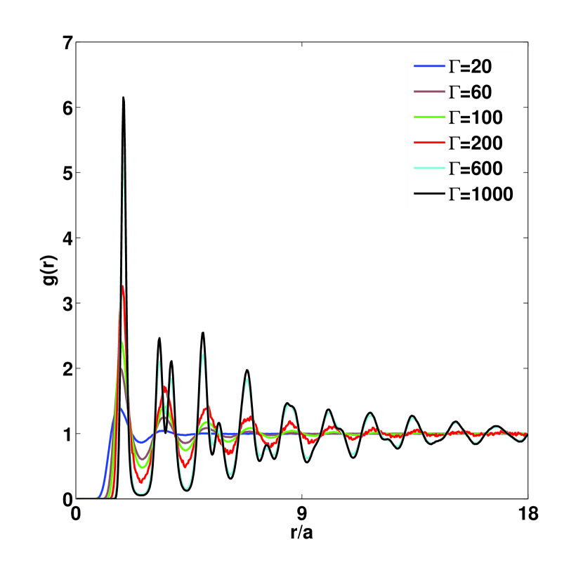
Figure 1: Radial distribution function $g(r)$ as a function of the reduced distance $r/a$ for $\kappa=1.0$, $\gamma=0.06$, and $\Gamma=20$, 60, 100, 200, 600, and 1000, corresponding to the increasing hight of the principal peak, respectively.

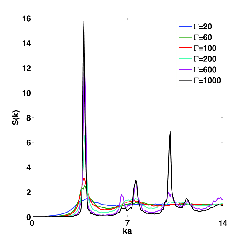
Figure 2: Static structure factor $S(k)$ as a function of the reduced wave-number $ka$ for $\kappa=1.0$, $\gamma=0.06$, and $\Gamma=20$, 60, 100, 200, 600, and 1000, corresponding to the increasing hight of the principal peak, respectively.

As described above, both the static structure factor $S(k)$ and the second frequency moments can be calculated from the equilibrium RDF $g(r)$, which is shown in Fig. 1 for several values of $\Gamma$. However, there are significant difficulties related to using $S(k)$ for modeling the dispersion relation of the longitudinal mode at long wavelengths. Namely, when $S(k)$ is calculated from the RDF, its small-$k$ values exhibit a very strong dependence on the fluctuations appearing in the simulation due to the finite number of dust particles [34]. This is expected to give rise to rather noisy dispersion curves, especially in the situations characterized by short relaxation times when the dispersion is dominated by the frequency $\omega_{0}(k)$ defined in Eq. (7jnq). To remedy the situation to some extent, we resort to calculating $S(k)$ directly from the simulation data by using the long time average of the Fourier transformed particle density in equilibrium, as follows

$$S(k)=\langle\rho^{*}(\mathbf{k})\rho(\mathbf{k})\rangle,$$ (7jnsy)

where

$$\rho(\mathbf{k})=\frac{1}{\sqrt{N}}\sum^{N}_{i=1}e^{i\mathbf{k}\cdot\mathbf{r}_{i}}.$$ (7jnsz)

In Fig. 2, we show the thus obtained results for $S(k)$ for several $\Gamma$ values, and note that the peak structures in that figure were found to be identical to those arising in $S(k)$ computed from the corresponding RDFs in Fig. 1.

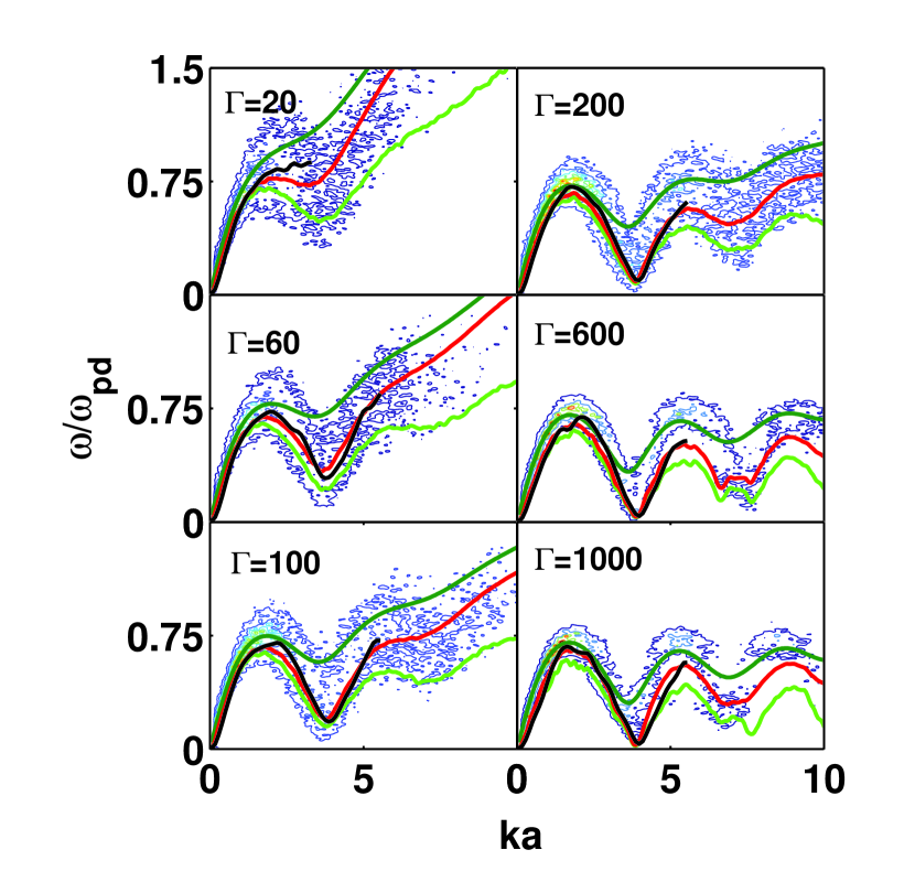
Figure 3: Longitudinal wave dispersion curves against simulation spectra for $\kappa=1.0$, $\gamma=0.06$, and $\Gamma=20$, 60, 100, 200, 600, and 1000. The upper (dark green), middle (red) and the lower (light green) solid curves represent the exponential model with an infinitely long, finite, and vanishing relaxation times, respectively. The thick solid (black) curve represents the Gaussian model for wave-numbers $ka<6$.

In Fig. 3 we show the simulation data for the spectral density of the longitudinal mode, along with the dispersion curves from the exponential model, represented by three solid curves corresponding to, in descending order, infinitely long, finite, and vanishing relaxation times $\tau_{l}$. Also shown in Fig. 3 by a thick black solid line is the dispersion curve obtained from the Gaussian model with the second and fourth frequency moments evaluated from Eq. (7a) with $n=1$ and 2, respectively, where $P_{l}(k,\omega)$ was taken directly from the simulation data for spectral density. While the three curves for the exponential model extend over the full range of wave-numbers shown in Fig. 3, the results for the Gaussian model are shown over a reduced range of wave-numbers covering the first Brillouin zone only, $ka<6$, because computations of the frequency moments via Eq. (7a) were hampered by a significant noise in the simulation spectra at larger wave-numbers and lower coupling strengths.

One notices in Fig. 3 that, for the exponential model with vanishing relaxation time (or, equivalently, the delta-function model), the resulting dispersion relation, $\omega=\omega_{0}(k)$ with $\omega_{0}(k)$ given in Eq. (7jnq), displays some noise coming from the simulation data via Eq. (7jnsy). We found this noise to be significantly weaker than the noise arising when $S(k)$ is calculated from the RDF. On the other hand, as the longitudinal relaxation time $\tau_{l}$ increases in the exponential model, there is a relative increase in the contribution of the second frequency moment $\langle\omega^{2}_{l}(k)\rangle$, which, when evaluated from the RDF via Eq. (7h), exhibits a much smoother $k$ dependence than $\omega_{0}(k)$ with $S(k)$ evaluated from Eq. (7jnsy).

As mentioned before, the dispersion relation for finite values of the relaxation time $\tau_{l}$ in the exponential model for the longitudinal viscosity memory function is obtained from the peak positions in the spectral density given by Eq. (7jnp) with Eqs. (7jnsa), (7jnsb), (7jnq), and (7jna). We have chosen the values of $\tau_{l}$ which provide the best fit to the peaks in the simulation spectral densities, and we have found $\tau_{l}$ to be a relatively weak function of $\Gamma$ that may be reasonably well approximated by

$$\tau_{l}(\Gamma)=\cases{0.769&for $\Gamma\leq 60$\\ 1.000&for $60<\Gamma\leq 200$\\ 1.333&for $200<\Gamma\leq 1000$.\\ }$$ (7jnsaa)

We emphasize that the quality of our choice of the values for $\tau_{l}$ in the exponential model is confirmed through a close agreement with the dispersion curves from the Gaussian model for wave-numbers in the first Brillouin zone, as displayed in Fig. 3.

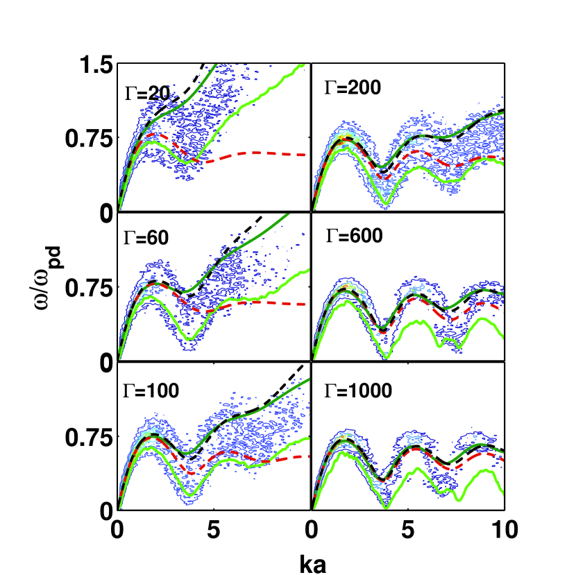
Figure 4: Longitudinal wave dispersion curves against simulation spectra for $\kappa=1.0$, $\gamma=0.06$, and $\Gamma=20$, 60, 100, 200, 600, and 1000. The upper (black) and the lower (red) dashed curve represent the results from the EQLCA and QLCA models, respectively. The upper (dark green) and the lower (light green) solid curves represent the exponential model with an infinitely long and vanishing relaxation times, respectively.

It is worth mentioning that the extreme cases of the exponential model, corresponding to the limits $\tau_{l}\to 0$ and $\tau_{l}\to\infty$, yield two parameter-free dispersion relations for the longitudinal mode, $\omega=\omega_{0}(k)$ and $\omega=\omega^{l}_{\infty}(k)$, respectively. Remarkably, it is noticed in Fig. 3 that these two dispersion relations provide good account of the simulation data by straddling the thermal noise, seen in the recorded spectra at the low-to-medium $\Gamma$ values. Moreover, at the medium-to-high $\Gamma$ values, one notices that $\omega=\omega_{0}(k)$ closely follows the dispersion relation from the Gaussian model for the wave-numbers in the first Brillouin zone and, in particular, reproduces the near-vanishing of frequency at around $ka\approx 4$ for $\Gamma=600$ and 1000. This is somewhat surprising, given that the delta-function model is stretched well into the condensed state at those two coupling strengths.

We further compare in Fig. 4 the dispersion relations $\omega=\omega_{0}(k)$ and $\omega=\omega^{l}_{\infty}(k)$ (shown by the upper and lower solid curves, respectively) with the results from the QLCA model [24], shown by the lower dashed curve. It is immediately obvious that the QLCA dispersion does not reproduce the direct thermal effect, which is responsible for a quasi-linear increase in the peak frequencies of the simulation spectra at higher wave-numbers and lower coupling strengths. In a previous work, we have shown that this deficiency can be easily rectified by a simple extension of the QLCA model, labeled as the EQLCA model in Ref.[22], which is shown by the upper dashed curve in Fig. 4. One notices a surprisingly good agreement between the EQLCA dispersion relation and the curve $\omega=\omega^{l}_{\infty}(k)$ from the exponential model for $\tau_{l}\to\infty$. While an agreement with the QLCA dispersion relation was expected at the higher $\Gamma$ values and lower $k$ values owing to the fact that the QLCA model inherently assumes $\omega\tau_{l}\gg 1$ [35] and the direct thermal effect is relatively weak at low $k$ and high $\Gamma$ values [22], it is remarkable how the parameter-free dispersion relation $\omega=\omega^{l}_{\infty}(k)$ provides justification for the empirically derived EQLCA model over the broad ranges of wavenumbers and coupling strengths.

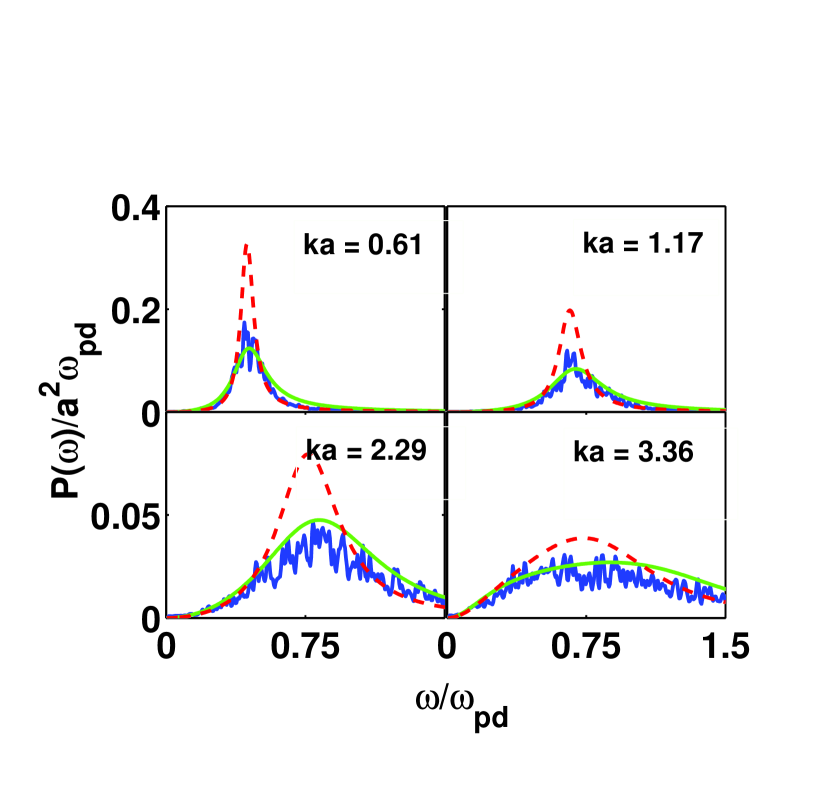
Figure 5: Longitudinal spectral density profile curves versus reduced frequency $\omega/\omega_{pd}$ for $\kappa=1.0$, $\gamma=0.06$, $\Gamma=20$, and $ka=0.61,1.17,2.29$, and 3.36. Simulation data are shown by the noisy (blue) solid curve, exponential model with finite relaxation time is represented by the dashed (red) curve, and the Gaussian model is represented by the smooth solid (green) curve.

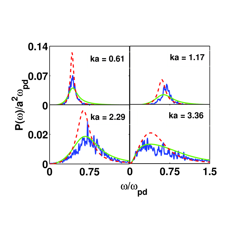
Figure 6: The same as Fig. 5, but for $\Gamma=60$.

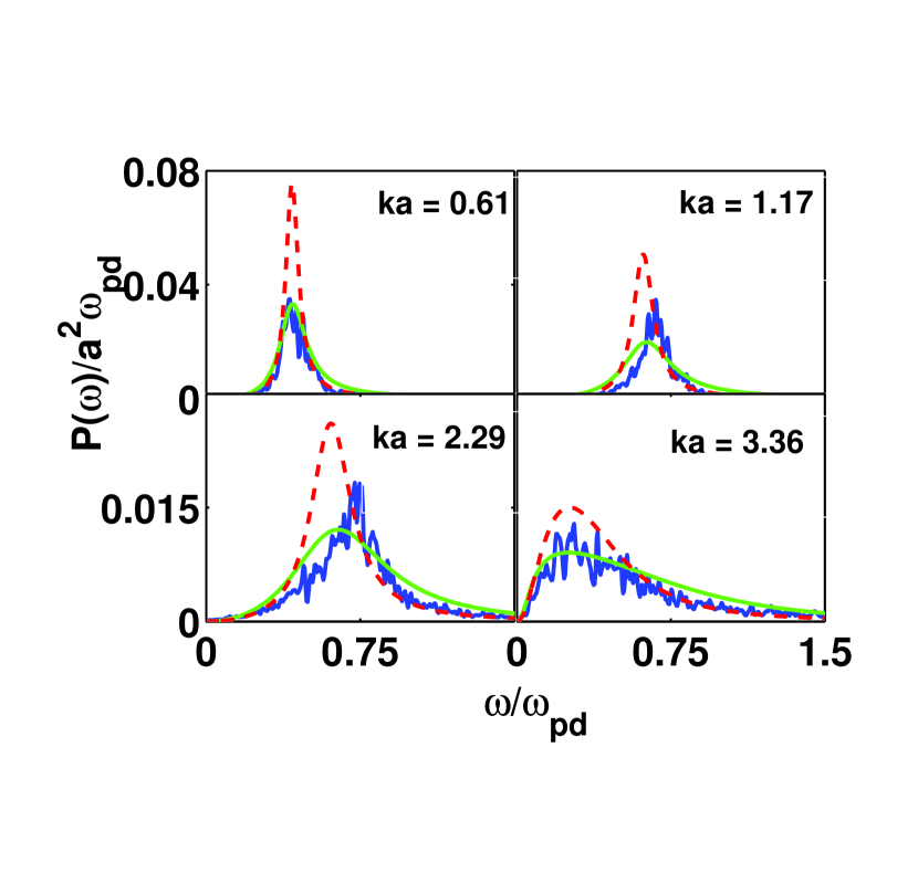
Figure 7: The same as Fig. 5, but for $\Gamma=100$.

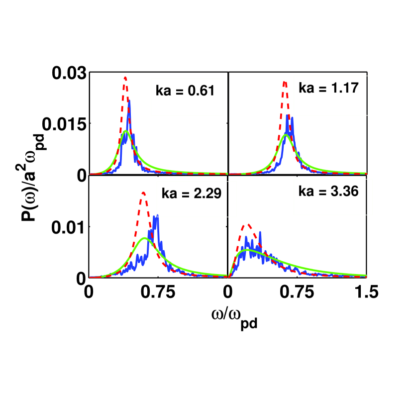
Figure 8: The same as Fig. 5, but for $\Gamma=200$.

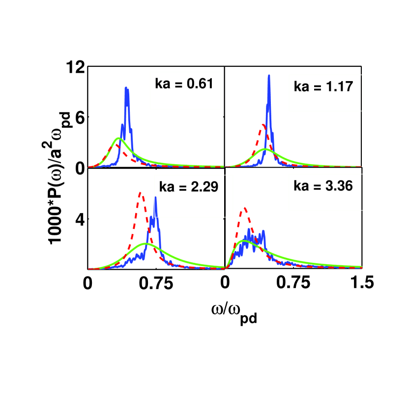
Figure 9: The same as Fig. 5, but for $\Gamma=600$.

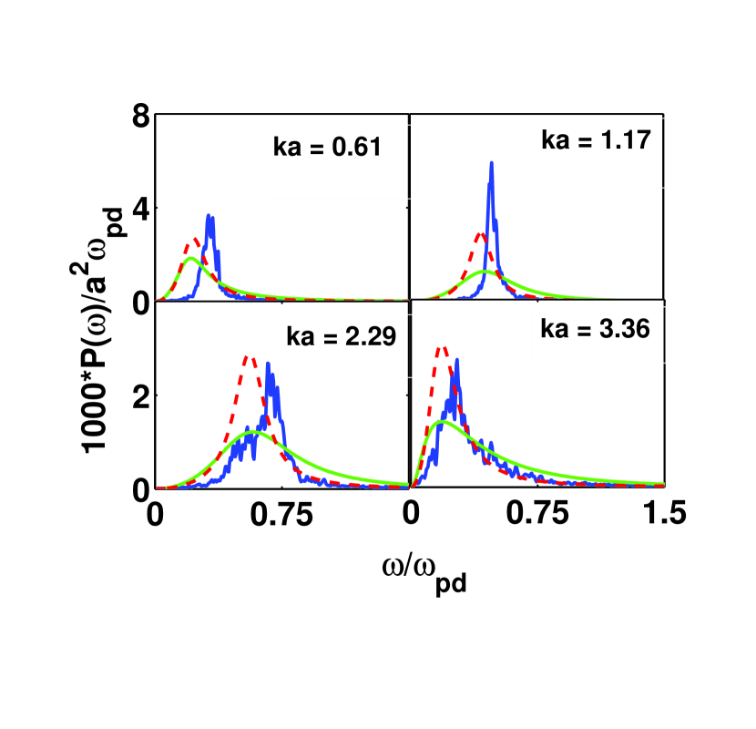
Figure 10: The same as Fig. 5, but for $\Gamma=1000$.

We next compare the performances of the exponential model with finite relaxation time $\tau_{l}$ from Eq. (7jnsaa) and the Gaussian model with the frequency moments evaluated from the simulation spectra via Eq. (7a) by using these two models in Eq. (7jnp) to predict the frequency dependent spectral profiles at several fixed wave-numbers. Given that the half-width at half-maximum (HWHM) of these profiles may be directly related to the wave-number dependent damping rate of the longitudinal DAW mode, in this way we demonstrate the advantage of using the memory function formalism within the GH model in tackling the difficult issue of damping of the collective excitation modes in dusty plasmas.

Specifically, we show in Figs. 5-10 the frequency dependencies obtained from the spectral density in Eq. (7jnp) with the exponential and the Gaussian models for four wave-numbers, $ka=0.61,1.17,2.29$, and 3.36, and compare them with the corresponding profiles of the simulation spectral density for $\Gamma=$ 20, 60, 100, 200, 600, and 1000, respectively. One notices in Figs. 5-10 a fair agreement between the simulation data and both GH models, which is especially good for lower $\Gamma$ values where the hydrodynamic regime is expected to be more pronounced, while for very high coupling strengths, say, $\Gamma>200$, the agreement begins to deteriorate. Comparison of both GH models with the simulation data may be considered fairly reasonable, even at high coupling strengths where the hydrodynamic model has been stretched well into the crystalline state.

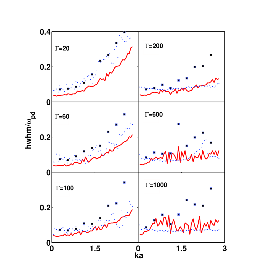
Figure 11: Half-width at half maximum of the spectral profile curves versus the reduced wave-number $ka$ for $\kappa=1.0$, $\gamma=0.06$, and $\Gamma=20$, 60, 100, 200, 600, and 1000, with the (blue) dots representing the simulation data, the (red) noisy solid curve representing the exponential model with finite relaxation time, and the squares representing the Gaussian model.

Finally, in Fig. 11, we show a comparison between the wave-number dependent HWHM values, obtained from the simulation spectral density profiles and from Eq. (7jnp) where we used both the exponential model with finite $\tau_{l}$ values given in Eq. (7jnsaa), and the Gaussian model with the frequency moments evaluated from the simulation spectra via Eq. (7a). One notices that all three sets of data are noisy due to the noise in the simulation spectra (one recalls that, in the case of the exponential model, the noise stems from $\omega_{0}(k)$ with $S(k)$ evaluated from Eq. (7jnsy)). As expected, the HWHM values from the Gaussian model are systematically somewhat larger than those from the exponential model, but they are both seen to be in reasonably good agreement with the simulation data, even though the agreement becomes blurred by the increased noise at the highest $\Gamma$ values, say $\Gamma>200$. One also notices in Fig. 11 that all damping rates roughly follow a quadratic dependence on $k$, with increasing opening of the parabola as $\Gamma$ gama increases, and with the limiting value as $k\to 0$ being close to the damping rate due to the neutral drag, given by $\gamma/2=0.03$.

4.2 Transverse Wave Mode

Transverse, or shear waves are expected to only exist for higher coupling strengths $\Gamma$ [14, 8]. In the following we compare the simulation results with the GH approach for a typical case of $\Gamma=100$.

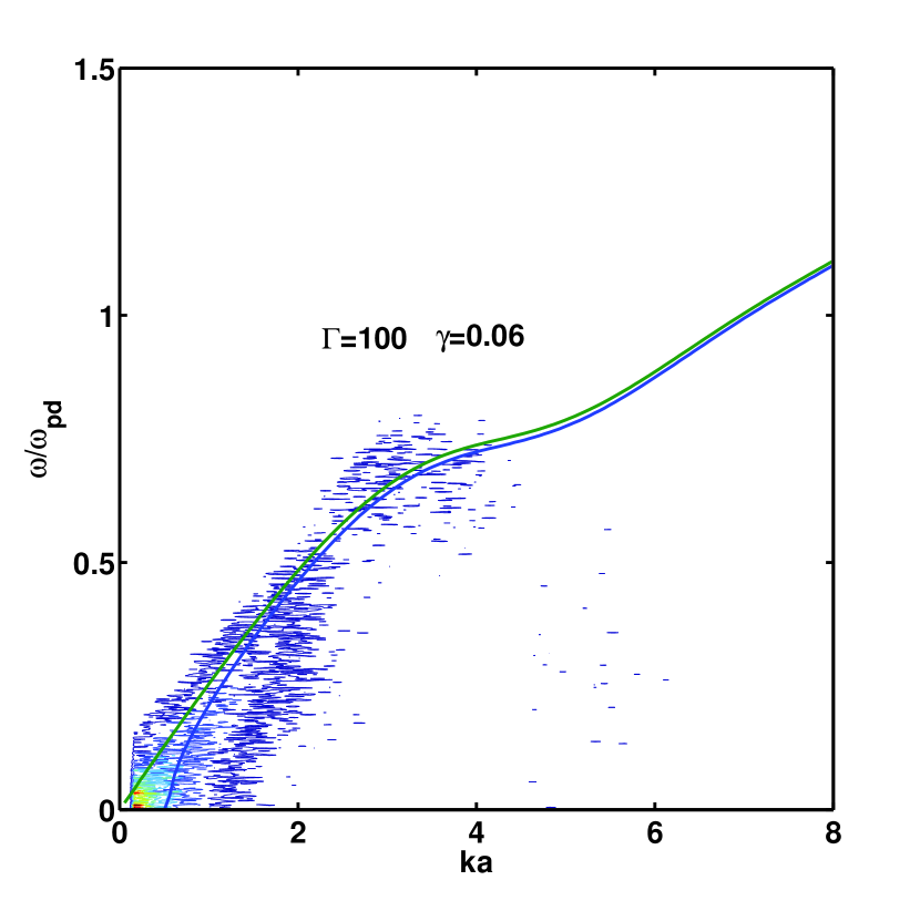
Figure 12: Transverse wave dispersion curves against the simulation spectra for $\kappa=1.0$, $\gamma=0.06$, and $\Gamma=100$, with the upper solid (green) curve and the lower solid (blue) curve representing the exponential model with an infinitely long and finite relaxation times, respectively.

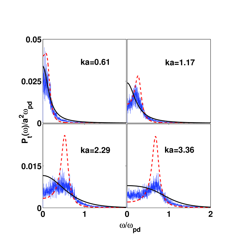
Figure 13: Transverse spectral density profile curves versus reduced frequency $\omega/\omega_{pd}$ for $\kappa=1.0$, $\gamma=0.06$, $\Gamma=100$, and $ka=0.61,1.17,2.29$, and 3.36. Simulation data are shown by the noisy (blue) solid curve, exponential model with finite relaxation time is represented by the dashed (red) curve, and the Gaussian model is represented by the smooth solid (black) curve.

Using Eq. (7i) to evaluate the second frequency moment from the RDF, we have obtained a dispersion relation from the peak positions of the spectral density in Eq. (7jnr) for the exponential model with $\tau_{t}=5.0$ (note that typical values of $\tau_{t}$ for the transverse mode are generally found to be larger than those for the longitudinal mode, in agreement with the remarks of Boon and Yip [26]). The results are shown in Fig. 12, along with the dispersion relation in the limit of infinite relaxation time, $\tau_{t}\to\infty$, given by $\omega=\omega^{t}_{\infty}(k)$ with Eq. (7jnsv), and are compared with the simulation spectrum for $\Gamma=100$. Both theoretical dispersion curves show good agreement with the simulation data for $ka<4$ and, while the simulation spectrum is not conclusive about the cutoff wave-number, the model with finite $\tau_{t}$ clearly exhibits a cutoff at $k_{c}\approx 0.5/a$ [14, 8].

Further, several profile plots of the spectral density are shown in Fig. 13 for $\Gamma=100$, where the results from Eq. (7jnr) for both the exponential model with $\tau_{t}=5.0$ and the Gaussian model with the frequency moments evaluated from the simulation data via Eq. (7a) are compared with the simulation profiles for $ka=0.61,1.17,2.29$, and 3.36. One notices that the agreement of the exponential model with the simulation spectral profiles is quite satisfactory for the lower two wave-numbers, but the simulation profiles at the two higher wave-numbers are seen to be much broader than the corresponding peaks from the exponential model. On the other hand, the Gaussian model does not reproduce the dispersion of the transverse mode at all, since the corresponding profile curves peak at zero frequency for all wave-numbers, as displayed in Fig. 13. Nevertheless, the broadening of the simulation profiles at the two higher wave-numbers in Fig. 13 seems to be better echoed by the Gaussian than by the exponential spectral profile curves.

5 Concluding Remarks

We have carried out Brownian Dynamics simulation of a 2D layer of strongly-coupled dusty plasma and extracted the equilibrium radial distribution function, static structure factor, and the spectral densities for both the longitudinal and transverse dust acoustic wave modes.

We have then shown that the memory function formalism of the theory of generalized hydrodynamics provides good semi-analytic results to model these wave modes. In particular, following the approach of Boon and Yip[26], we have developed an exponential model for the viscosity memory functions that satisfies the second frequency sum rule with the relaxation time being used as a fitting parameter. With such exponential model we have obtained good fits to the simulation data for the longitudinal dispersion curves over a wide range of coupling strengths, $20\leq\Gamma\leq 1000$, as well as reasonable match with the spectral density profiles for several values of the wave-number $k$. Next, we have extended the theory in a straightforward manner to satisfy the third and fourth frequency sum rules, providing a parameter-free Gaussian model for the viscosity memory function. The results using this model provided a successful test for our choice of the relaxation time in the exponential model in modeling both the dispersion relations and the spectral density profiles.

Moreover, we pointed out that the limits of an infinitely long and infinitesimally short relaxation times in the exponential model represent two parameter-free models that are fully determined by the equilibrium radial distribution function and the static structure factor of the system. It was then shown that these two limits provide good upper and lower bounds for the thermal noise observed in the simulation spectra for the longitudinal mode. Comparisons of the dispersion relations obtained from these two limits of the exponential model with the dispersion relations obtained from both the Quasi-localized charge approximation (QLCA) and the extended QLCA (EQLCA) showed that the limit of an infinitely long relaxation time reproduces remarkably well all the features of the EQLCA model, including the direct thermal effect. On the other hand, the limit of an infinitesimally short relaxation time was found to reproduce the near-vanishing of the dispersion relation, which is seen in the simulation spectra at certain short wave-lengths for large coupling strengths, but is not reproduced by the QLCA group of results.

In addition, we have also tested the memory function formalism within the theory of generalized hydrodynamics against the simulation results obtained for transverse wave modes at the coupling strength of $\Gamma=100$, and found that the exponential model with relaxation time used as a fitting parameter can provide a reasonable estimate for the wave dispersion relation, including the appearance of a cutoff wave-number. Both the peak positions and the widths in the spectral density profiles from the simulation were well reproduced by the exponential model at long wavelengths, whereas the broadening of these spectra at short wavelengths was better echoed by the Gaussian model.

The most important finding of the present analysis is that the wave-number dependent damping rates, which were extracted from the simulation spectra, were found in good agreement with the results from both the exponential and Gaussian models, testifying to the strengths and potentials of using the memory-function formalism within the GH theory in describing the damping of the longitudinal dust acoustic wave in strongly-coupled dusty plasmas.

Finally, we have included the effect of neutral drag due to the collisions of dust particle with neutral molecules in the background plasma via a (local in time) drag coefficient. While we did not find that the neutral drag affects our modeling of dispersion relations for both the longitudinal and transverse waves in any significant way, the overall damping rates for the longitudinal wave showed possibly important roles of the neutral drag at long wavelengths and high coupling strengths where viscous damping is expected to be reduced. This aspect of the GH theory shall be studied in future work.

In conclusion, the memory function formalism of the generalized hydrodynamics provides a very promising route to analytical modeling of spectral density of collective modes in strongly coupled 2D dusty plasmas and, in particular it demonstrates a good account of viscoelastic effects which are not well described by other analytical methods.

This work was supported by the Natural Sciences and Engineering Research Council of Canada. LJH would thank M. S. Murillo and V. Nosenko for valuable discussions.

Appendix A Frequency sum rules

Initial-value properties of the current density auto-correlation functions are related to the even-order frequency moments via [26]

$$\langle\omega^{2n}_{l,t}(k)\rangle=(-1)^{n}\left[\frac{\partial^{2n}}{\partial t^{2n}}C_{l,t}(k,t)\right]_{t=0},$$ (7jnsab)

whereas all odd-order moments must vanish. We extend here the development outlined by Boon and Yip [26] by introducing the third and fourth frequency sum rules into the GH theory of spectral density. Since these sum rules are used to fix the short time properties of the model memory functions, we may again initially neglect the neutral drag.

To illustrate this procedure for the longitudinal mode, we differentiate Eq. (7jl) twice to obtain the third derivative as

$$\frac{\partial^{3}}{\partial t^{3}}C_{l}(k,t)=-\frac{k^{2}v_{th}^{2}}{S(k)}\frac{\partial}{\partial t}C_{l}(k,t)-k^{2}\int_{0}^{t}dt^{\prime}\ C_{l}(k,t^{\prime})\frac{\partial^{2}}{\partial t^{2}}\phi_{l}(k,t-t^{\prime})$$

$$-k^{2}\left[C_{l}(k,t^{\prime})\frac{\partial}{\partial t}\phi_{l}(k,t-t^{\prime})\right]_{t^{\prime}=t}-k^{2}\phi_{l}(k,0)\frac{\partial}{\partial t}C_{l}(k,t),$$ (7jnsac)

which on evaluating at $t=0$, yields

$$\left[\frac{\partial^{3}}{\partial t^{3}}C_{l}(k,t)\right]_{t=0}=-k^{2}\left[C_{l}(k,t^{\prime})\frac{\partial}{\partial t}\phi_{l}(k,t-t^{\prime})\right]_{t^{\prime}=t=0}.$$ (7jnsad)

Since the third moment must vanish, we have the condition

$$-k^{2}C_{l}(k,0)\left[\frac{\partial}{\partial t}\phi_{l}(k,t-t^{\prime})\right]_{t^{\prime}=t=0}=0,$$ (7jnsae)

showing that the first derivative of the longitudinal viscosity memory function must vanish at initial time. This is to be expected because a memory function should be viewed as being just another time auto-correlation function with vanishing derivatives of odd order at the initial time [26]. Next, evaluating the fourth moment we find

$$\frac{\partial^{4}}{\partial t^{4}}C_{l}(k,t)=-\frac{k^{2}v_{th}^{2}}{S(k)}\frac{\partial^{2}}{\partial t^{2}}C_{l}(k,t)-k^{2}\int_{0}^{t}dt^{\prime}\ C_{l}(k,t^{\prime})\frac{\partial^{3}}{\partial t^{3}}\phi_{l}(k,t-t^{\prime})$$

$$-k^{2}\left[C_{l}(k,t^{\prime})\frac{\partial^{2}}{\partial t^{2}}\phi_{l}(k,t-t^{\prime})\right]_{t^{\prime}=t}-k^{2}\left[\frac{\partial}{\partial t}C_{l}(k,t)\frac{\partial}{\partial t}\phi_{l}(k,t-t^{\prime})\right]_{t^{\prime}=t}$$

$$-k^{2}\phi_{l}(k,0)\frac{\partial^{2}}{\partial t^{2}}C_{l}(k,t).$$ (7jnsaf)

Again setting $t=0$ we obtain,

$$\left[\frac{\partial^{4}}{\partial t^{4}}C_{l}(k,t)\right]_{t=0}= -\frac{k^{2}v_{th}^{2}}{S(k)}\left[\frac{\partial^{2}}{\partial t^{2}}C_{l}(k,t)\right]_{t=0}$$ (7jnsag)

$$-k^{2}C_{l}(k,0)\left[\frac{\partial^{2}}{\partial t^{2}}\phi_{l}(k,t-t^{\prime})\right]_{t^{\prime}=t=0}$$

$$-k^{2}\phi_{l}(k,0)\left[\frac{\partial^{2}}{\partial t^{2}}C_{l}(k,t)\right]_{t=0}.$$

Substituting $\phi_{l}(k,0)$ from Eq. (7jna) and invoking Eq. (7jnsab) with $n=1$ and 2, we obtain Eq. (7jnsw) in the main text.

References

References

- [1] P.K. Shukla and A.A. Mamun, Introduction to Dusty Plasma Physics (Institute of Physics, Bristol, 2002).
- [2] P.K. Shukla and B. Eliasson, Rev. Mod. Phys. 81, 25 (2009).
- [3] G.E. Morfill and A.V. Ivlev, Rev. Mod. Phys. 81, 1353 (2009).
- [4] J. B. Pieper, and J Goree, Phys. Rev. Lett. 84, 6026 (1996).
- [5] A. Homann, A. Melzer, S. Peters et al., Phys. Rev. E 56, 7138 (1997); Phys. Lett. A 242, 173 (1998).
- [6] S. Nunomura, J. Goree, S. Hu, X. Wang, A. Bhattacharjee, and K. Avinash, Phys. Rev. Lett. 89, 035001 (2002).
- [7] S. Nunomura, S. Zhdanov, D. Samsonov, and G. Morfill, Phys. Rev. Lett. 94, 045001 (2005).
- [8] V. Nosenko, J. Goree, and A. Piel, Phys. Rev. Lett. 97, 115001 (2006).
- [9] L. Couedel, V. Nosenko, S. K. Zhdanov, A. V. Ivlev, H. M. Thomas, and G. E. Morfill, Phys. Rev. Lett. 103, 215001 (2009).
- [10] L. Couedel, V. Nosenko, A. V. Ivlev, S. K. Zhdanov, H. M. Thomas, and G. E. Morfill, Phys. Rev. Lett. 104, 195001 (2010).
- [11] N. N. Rao, P. K. Shukla, and M. Y. Yu, Planetary and Space Science 38, 543 (1990).
- [12] X. Wang and A. Bhattacharjee, Phys. Plasmas 4, 3759 (1997).
- [13] P.K. Kaw and A. Sen, Phys. Plasmas 5, 3552 (1998).
- [14] M.S. Murillo, Phys. Rev. Lett. 85, 2514 (2000).
- [15] K.I. Golden and G.J. Kalman, Phys. Plasmas 7, 14 (2000).
- [16] G. Kalman, M. Rosenberg, and H. E. DeWitt, Phys. Rev. Lett. 84, 6030 (2000)
- [17] H. Ohta and S. Hamaguchi, Phys. Rev. Lett. 84, 6026 (2000).
- [18] X. Wang, A. Bhattacharjee, and S. Hu, Phys. Rev. Lett. 86, 2569 (2001).
- [19] S. Zhdanov, S. Nunomura, D. Samsonov, and G. Morfill, Phys. Rev. E 68, 035401(R) (2003).
- [20] G. J. Kalman, P. Hartmann, Z. Donkó and M. Rosenberg, Phys. Rev. Lett. 92, 065001 (2004).
- [21] A. Piel and J. Goree, Phys. Plasmas 13, 104510 (2006).
- [22] L. J. Hou, Z.L. Miskovic, A. Piel, and M.S. Murillo, Phys. Rev. E 79, 046412 (2009).
- [23] L. J. Hou, P. K. Shukla, A. Piel, Z. L. Miskovic, Phys. Plasmas 16, 073704 (2009).
- [24] Z. Donko, G.J. Kalman, and P. Hartmann, J. Phys.: Cond. Matt. 20, 413101 (2008).
- [25] N. Ailawadi, A. Rahman, and R. Zwanzig, Phys. Rev. A 4, 1616 (1971).
- [26] J.P. Boon and S. Yip, Molecular Hydrodynamics (McGraw-Hill, New York, 1980).
- [27] J.P. Hansen and I.R. McDonald, Theory of Simple Liquids (Academic Press, London, 1986).
- [28] A. Piel, V. Nosenko and J. Goree, Phys. Plasmas 13, 042104 (2006).
- [29] W. Hess and R. Klein, Adv. Physics 32, 173 (1983).
- [30] M.S. Murillo, Phys. Plasmas 7, 33 (2000).
- [31] L. J. Hou, Z. L. Miskovic, A. Piel and P. K. Shukla, Phys. Plasmas 16, 053705 (2009); L. J. Hou and Z. L. Miskovic, arXiv:0806.3912.
- [32] N. Upadhyaya, L. J. Hou, and Z. L. Miskovic, Phys. Lett. A 374, 1379 (2010).
- [33] Z. Donko, J. Goree, P. Hartmann, and B. Liu, Phys. Rev. E 79, 026401 (2009).
- [34] P. Hartmann, G.J. Kalman, Z. Donko, and K. Kutasi, Phys. Rev. E 72, 026409 (2005).
- [35] P.K. Kaw, Phys. Plasmas 8, 1870 (2001).