The overlap parameter across an inverse first order phase transition in a 3D spin-glass

Abstract

We investigate the thermodynamic phase transition taking place in the Blume-Capel model in presence of quenched disorder in three dimensions (3D). In particular, performing Exchange Montecarlo simulations, we study the behavior of the order parameters accross the first order phase transition and its related coexistence region. This transition is an Inverse Freezing.

1 Introduction

In the present paper, we will consider the Blume-Capel[1, 2, 3] model with quenched disorder (BC-random)[4, 5, 6, 7]: a spin-glass model with bosonic spin$-1$ variables ($s_{i}=-1,0,+1$). BC-random is one of the simplest spin glass models that displays an Inverse Transition (IT)[8]. By IT we mean a reversible transition occurring between phases whose entropic content is in the inverse order relation relatively to standard transitions. The case - already hypothesized by Tammann more than a century ago [9] - of “ordering in disorder” taking place in a crystal solid that liquefies on cooling, is generally termed inverse melting. The IT phenomenon also includes the transformation involving amorphous solid phases, as that of a liquid vitrifying upon heating, and the term inverse freezing (IF) is somewhat used in the literature: both phases are disordered but the fluid appears to be the one with least entropic content. IT has been experimentally observed in many materials: some examples of inverse melting can be found in[10, 11, 12, 13, 14, 15, 16, 17, 18, 19, 20, 21, 22, 23], while IF takes place in[24, 25, 26]. The reason for these counter intuitive phenomenon is that a phase usually at higher entropic content happens to exist in very peculiar patterns such that its entropy actually decreases below the entropy of the phase normally considered the most ordered one[27, 28].
The Mean Field (MF) solution of the BC-random model in the Full Replica Symmetry Breaking (RSB) scheme[5, 6] predicts a phase diagram (fig. 1) with a second order transition line (between Spin-Glass (SG) and Paramagnet (PM) phase) ending in a tricritical point, where a first order phase transition line starts, and from where a phase coexistence region departs.
We stress that the transition is first order in the thermodynamic sense, with latent heat and is not related to the so-called random first order transition[29] occurring in MF models for structural glasses. Furthermore, the first order transition is characterized by the phenomenon of IF [30, 31]: the low temperature phase is PM, with a lower entropy than the SG phase, and the transition line develops a reentrance.
In the present work we will study the behavior of the 3D BC-random model on a cubic lattice with nearest-neighbor quenched interaction. The nature of the phases that appear in the phase diagram, in particular across the IF First Order Phase Transition (FOPT), is studied through the shape of the order parameters distributions: this qualitative method allow us to understand, in a very simple way, the fundamental phenomenology that drives the IF scenario. Other results on the same model have been presented in [8, 32].

2 Model and Observables

The Hamiltonian of the BC-random is defined as follows

$${\mathcal{H}}_{J}[s]=-\sum_{(i,j)}J_{ij}s_{i}s_{j}+D\sum_{i}s_{i}^{2}$$ (1)

where $({i}{j})$ indicates ordered couples of nearest-neighbor sites, and $s_{{i}}=-1,0,+1$ are spin$-1$ variables lying on a cubic lattice of size $N=L^{3}$ with Periodic Boundary Condition. The external crystal field $D$ plays the role of a chemical potential. Random couplings $J_{{i}{j}}$ are independent identically distributed as

$$P(J_{{i}{j}})=\frac{1}{2}\delta(J_{{i}{j}}-1)+\frac{1}{2}\delta(J_{{i}{j}}+1).$$ (2)

We simulate two real replicas of the system and define the overlap, i.e. the order parameter usually characterizing the SG transition, as

$$q^{(J)}\equiv\frac{1}{N}\sum_{{i}}\langle s^{(1)}_{{i}}s^{(2)}_{{i}}\rangle$$ (3)

where $\langle\ldots\rangle$ is the thermal average. If a thermodynamic first order phase transition occurs, with latent heat, the most significant order parameter that drives the transition is the density $\rho$ of magnetically active ($|s_{i}|=1$) sites:

$$\rho^{(J)}=\frac{1}{N}\sum_{{i}}\langle s^{2}_{{i}}\rangle\;.$$ (4)

The apex $J$ recalls us that the values of the parameters depend on the particular realization of disorder ($\{J_{{i}{j}}\}$). All the information about the equilibrium properties of the system is in the knowledge of the following probability distribution functions (pdfs)

$$P(q) \equiv \overline{P_{J}(q)}=\overline{\left\langle\delta\left(q^{(J)}-\frac{1}{N}\sum_{i}s_{i}^{(1)}s_{i}^{(2)}\right)\right\rangle}$$ (5)

$$P(\rho) \equiv \overline{P_{J}(\rho)}=\overline{\left\langle\delta\left(\rho^{(J)}-\frac{1}{N}\sum_{{i}}s^{2}_{{i}}\right)\right\rangle}\;.$$

We denote by ${\overline{\phantom{(}\ldots\phantom{)}}}$ the average over quenched disorder. The dependence on the random couplings $J_{ij}$ is known to be self-averaging for the density probability distribution, but not for the overlap distributions $P_{J}(q)$, whose average over the quenched disorder in the thermodynamic limit is different from the thermodynamic limit of a single realization of random couplings[33]:

$$P(q) \equiv \lim_{N\to\infty}\overline{P_{J}(q)}\neq\lim_{N\to\infty}P^{(N)}_{J}(q)\,.$$ (6)

We can introduce the notion of active and inactive site: when $s_{i}=0$ the site is inactive; otherwise, if $s_{i}^{2}=1$, it can interact with its neighbors ($s_{i}$ is an active site): as we will see in the next sections the IF indeed takes place between a SG of high density to an almost empty PM. The few active sites practically do not interact with each other but almost exclusively with inactive neighbors and this induces zero magnetization and overlap. The corresponding PM phase at the same $D$ and high $T$ has, instead, higher density and the paramagnetic behavior is brought about by the lack of both magnetic order (zero magnetization) and blocked spin configurations (zero overlap), cf. Sec 3.

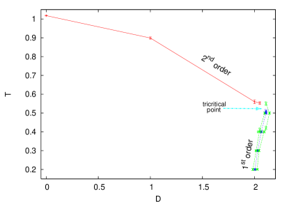
Figure 1: Left panel: the phase diagram of the BC model with quenched disorder for the fully-connected lattice with Gaussian distribuited random couplings (MF solution [5, 6]): the Second Order Phase Transition ends in a tricritical point where an Inverse Freezing First Order Phase Transition takes place. The variance of $P(J_{ij})$ in the MF model was $\propto 1/z$, $z$ being the number of sites connected to each spin. In the 3D model, where $z=6$ (right panel), a bimodal distribution has been chosen with variance $1$ rather than $\propto 1/6$.

3 Phase Transitions and Order Parameters

The equilibrium dynamics of the BC-random has been numerically simulated through Parallel Tempering (PT) technique: we have simulated in parallel the dynamic of the system at different values of $T$ and $D$. For the PT in $T$, the swap probability of two copies at $T$ and $T+\Delta T$ was:

$$P_{\mbox{swap}}(\Delta\beta)=\min\left[1,\exp\{\Delta\beta\Delta\mathcal{H}\}\right]\,.$$ (7)

While, for PT in $D$, two copies with $D$ and $D+\Delta D$ were exchanged with probability

$$P_{\mbox{swap}}(\Delta D)=\min\left[1,\exp\{\beta\Delta D\Delta\rho\}\right]\,.$$ (8)

We will present data of 3D systems studied with PT in $T$ at $D=0$, and in $D$ at $T=0.2,0.3,0.4,0.5$. At $D=0$ we simulated from $33$ to $40$ replicated copies $N_{T}$ at linear size $L=6,8,10,12$ (number of disordered sample: $N_{J}=2000$), for $D=0$ we simulated $N_{T}\in[20:33]$ at $L=16,20$ ($N_{J}\in[900:1500]$) and $N_{T}\in[17:22]$ at $L=24$ ($N_{J}\in[500:1000]$). For the PT cycles in $D$, $N_{D}\in[21:37]$, parallel replicas at different $D$ were simulated, for size $L=6,8,10,12$ and $15$ ($N_{J}=1000$). In the latter case, to resolve the coexistence region, varying $\Delta D$ were used, larger in the pure phases and progressively smaller approaching the transition. The number of Monte Carlo (MC) steps varies from $2^{15}$ to $2^{21}$ according to $L$ and to the lowest values of $T,D$ reached.
Thermalization has been cross checked by looking at: (i) the symmetry of the overlap distributions $P_{N,J}(q)$, (ii) the $t$-log behavior of the energy (when at least the last two points coincide), (iii) the lack of variation of each considered observable (e.g., $P(q),\,P(\rho)$) on logarithmic time-windows.

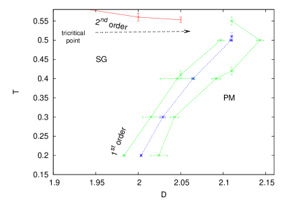
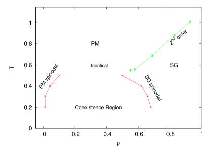
Figure 2: The phase diagrams of the BC model with quenched disorder in three dimension. In the left panel is shown the $T-D$ plane. The FOPT transition line develops a reentrance, it is an IT: decreasing the temperature the system leaves the SG phase and liquefies in a PM phase. In figure the spinodal lines (green) are reported and the blue line is the critical line of the FOPT. The arrow pointing to the region of the phase diagram where is located the tricritical point. In the right panel the $T-\rho$ plane is shown.

In fig. (2) the phase diagram of the model is shown: both in $T-D$ and in $T-\rho$ plane. The second order phase transition has already been studied in [8], details can be found in [32]. In short, by the study of the four-spins correlation function

$$C_{4}(x)\equiv\overline{\frac{1}{N}\langle\sum_{i}q_{i}^{(J)}q_{i+x}^{(J)}\rangle}=\overline{\frac{1}{N}\langle\sum_{i}s_{i}^{(1)}s_{i}^{(2)}s_{i+x}^{(1)}s_{i+x}^{(2)}\rangle}$$ (9)

we can introduce a correlation lenght $\xi(T,L)/L$ that is scale invariant at the critical point: this property allows to define a size-dependet $T_{c}(L)$. Finally, through Finite Size Scaling techniques, it is possible to calculate the critical temperature in the Thermodynamic Limit[34, 35].

The order parameter that drives the FOPT at finite $L$ is the density distribution $P(\rho)$: varying $D,T$, the system undergoes a transition with a discontinuous jump in $\rho$ (and, thus, in $q$). The system is in the coexistence region if $P(\rho)$ displays two peaks corresponding to the PM (low $\rho$) and SG (high $\rho$) phases. The first order transition line $D_{c}(L,T)$, is the locus of points where the two phases are equiprobable, i.e., the areas of the two peaks are equal [36]:

$$\int_{0}^{\rho_{0}}d\rho\,P(\rho)=\int_{\rho_{0}}^{1}d\rho\,P(\rho)$$ (10)

where $\rho_{0}\in[\rho_{PM}:\rho_{SG}]$ such that $P(\rho)=0$ (or minimal next to the tricritical point). In order to determine the transition point a method is to compare the areas under the distributions, cf. Eq (10). This is the point at which the configurations belonging to the SG phase and those belonging to the PM phase have the same statistical weight: they yield identical contribution to the partition function of the single pure phase, and the free energies of the two coexisting phases are equal. We work at finite T moving D in that region and this method works quite well for $T\leq 0.4$ because the two peaks are clearly separated as soon as they appear, cf. fig. (3). Determination of $D_{c}$ is robust against reasonable changes of $\rho_{0}$. At T=0.5 we have the problem that the distributions of the densities of the two phases are overlapping. In that case, seen the arbitrariness of choosing $\rho_{0}$, we actually determine the transition point as the D value at which the peaks have the same height.

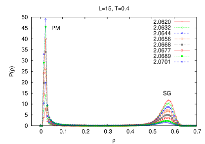
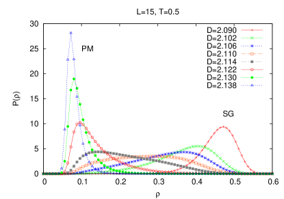
Figure 3: Density distribution $P_{L}(\rho)$, $L=15$, across the coexistence region at $T=0.4$ (left) and $T=0.5$ (right): two peaks develop at $\rho_{PM}$ and $\rho_{SG}$. As $D$ increases the thermodynamically relevant phase (lowest free energy) passes from SG to PM in a first order phase transition. The dominant phase correpsonds to the one with larger probability, i.e., larger intergral of the peak. As the peak at $\rho_{SG}$ vanishes the system is in a purely PM phase. At $T=0.5$ (right) a coninuum part between the SG and PM peaks appears: the distribution of the densities of two phases are overlapping.

To have a better confidence with the results, two other methods have been used to determine the first order transition. These are not plagued by the problem of dealing with overlapping distributions since they do only rely on averages. The methods are:

1. Equal distance: at a given T, we plot D versus average $\rho$, we extrapolate the $D(\rho)$ curves both from the PM and the SG phase ($D_{PM}(\rho)$ and $D_{SG}(\rho)$) and we make a Maxwell-like construction determining a value of $D_{c}$ at which

   $$\rho(D_{c})=\frac{1}{2}\left(\rho_{\rm PM}(D_{c})+\rho_{\rm SG}(D_{c})\right)\,.$$ (11)

2. Equal area: equivalently (the equivalence is in the thermodynamic limit) one can determine $D_{c}$ as the value at which

   $$\int_{D_{\rm SG}}^{D_{c}}\rho_{\rm PM}(D)dD+\int_{D_{c}}^{D_{\rm PM}}\rho_{\rm SG}(D)dD=\int_{D_{\rm SG}}^{D_{\rm PM}}\rho(D)dD$$ (12)

   where $D_{\rm SG}$ and $D_{\rm PM}$ are arbitrary, provided they pertain to the relative pure phases. The extrapolated, $\rho_{\rm PM}(D)$ ($\rho_{\rm SG}(D)$) is the inverse of the extrapolated curve $D_{\rm PM}(\rho)$ ($D_{\rm SG}(\rho)$). The curves are obtained by using all data, including those in the candidate coexistence region.

   We will show and compare in Sec. (3.2) the results obtained by these three methods.

3.1 Second Order Phase Transition

In fig. (4) (left panel) we report the distribution of overlap $P(q)$ for a system of linear size $L=16$ and $D=0$: it changes shape accross the second order phase transition[37] between the PM and SG phase from a Gaussian to a double peaked distribution

$$P_{SG}(q)\propto\delta(q-q_{EA})+\delta(q+q_{EA})+f(q,L)\;,$$ (13)

where $f(q,L)$ is a continuous function depending on the size. In the right panel of the figure we show the behavior of $P(\rho)$ at fixed values of the crystal field and several temperatures: decreasing the temperature, deep in the SG phase, the average number of active sites is close to one

$$\lim_{T\to 0}\overline{\langle\rho\rangle}=\int_{0}^{1}\,d\rho\,P(\rho,T)\,\rho\sim 1\,.$$ (14)

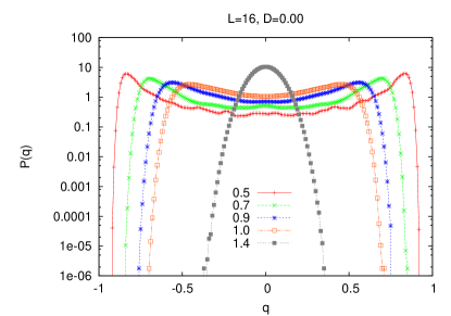
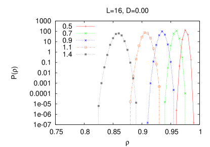
Figure 4: $P_{L}(q)$ and $P_{L}(\rho)$ for $L=16$ and $N_{J}=1500$ at $D=0.00$. Across the transition $P(q)$ (left panel) changes shape continuously from a Gaussian (in the high temperature phase) to, decreasing the temperature, a double peaked distribution with a continuum part between the peaks. In this region of the phase diagram the FOPT does not take place: $P(\rho)$ (right panel) does not change shape.

The distribution $P_{L}(\rho)$ does not change shape across this transition.

3.2 First Order Phase Transition

Beyond the tricritical point, FOPT takes place and the system undergoes a discontinuous transition between an “inactive” PM phase ($\overline{\langle\rho\rangle}\equiv\rho_{m}\sim 0$) and an “active” SG phase ($\rho_{m}\neq 0$). In the coexistence region, we can write the $P(q)$ as sum of two contributes:

$$P(q)=P_{SG}(q)+P_{PM}(q)\,.$$ (15)

For the PM contribution $P_{PM}(q)$ we have a Gaussian strongly peaked around $q=0$. The $P_{SG}(q)$ consists of a double peak (trivial) distribution with a continuum (non trivial) part between the two peaks, cf. Sec. 3.1.

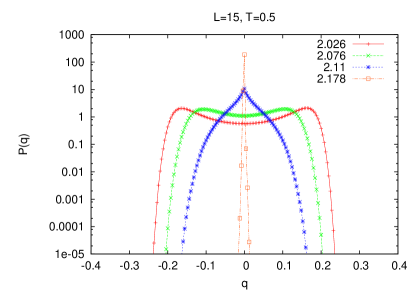
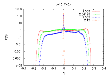
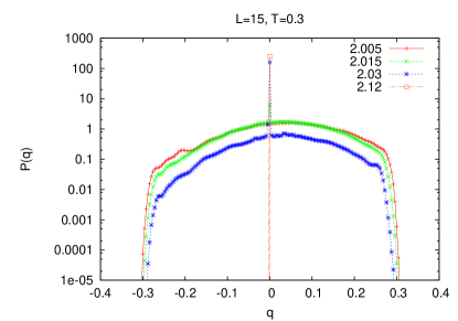
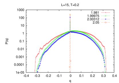
Figure 5: $P(q)$ across the FOPT at fixed $T$ and different $D$ values: we have a coexistence region between the phases SG and PM. The PM phase contributes to the $P(q)$ distribution with a delta function in $q=0$.

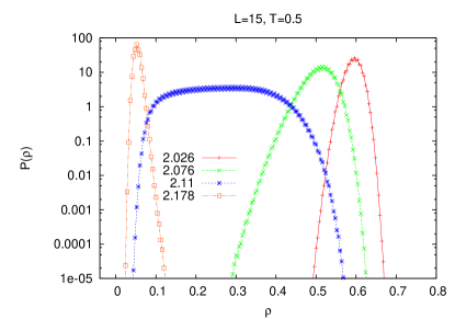
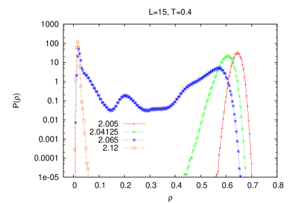
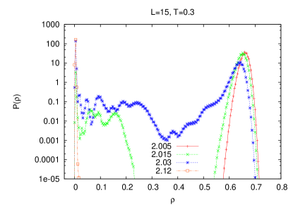
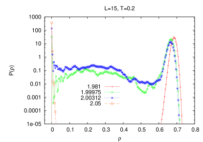
Figure 6: $P(\rho)$ during the FOPT: a double peak signal the coexistence of phases while, when the system is in a pure phase, we have a single peak.

In fig. (5) we show the behavior of $P(q)$ at different temperatures when the FOPT occurs. In the coexistence region, besides the double peak with a continuous part of the SG phase, a peak in $q=0$ appears due to the large density of empty sites.
As shown in fig. (2), cf. also Sec. 2, FOPT occurs as an IF: the PM phase riches of inactive sites, below the T-range at which a pure SG phase is present, becomes the low temperature (and less entropic) phase. This can be better observed in fig. (6) where $P(\rho)$ is represented at several values of $D$ through the transition. In table (1) the critical values of the FOPT reported are obtained by the equal weight, equal area and equal distance methods.

T	$D_{c}[P(\rho)]$	$D_{c}[\rho_{m}]$	$D_{c}[\mathcal{A}(\rho)]$	$D_{sp}(PM)$	$D_{sp}(SG)$
0.2	1.992(2)	1.998(3)	1.999(2)	1.98333(15)	2.0243(95)
0.3	2.032(2)	2.032(3)	2.030(1)	2.015(1)	2.043(5)
0.4	2.061(1)	2.060(2)	2.058(1)	2.046(2)	2.092(5)
0.5	2.107(1)	2.102(1)	2.102(2)	2.097(4)	2.143(4)

Table 1: Critical values of the field $D$ calculated through the equiprobability of the phases (eq. 9, blue line in the left panel of fig. (2)), the equal distance (eq. 10) and the equal area (eq. 11) respectively. In the last two columns are reported the spinodal lines $D_{sp}$ (green lines in the left panel of fog. (2)).

From the study of the shape of $P(\rho)$ in the different phases (high-T PM phase, SG phase and low-T PM phase), the 3D BC-random model, allows us to interpretate the IF scenario in a very intuitive picture. Starting from a point of the phase diagram (D,T) in the high temperature phase (high-T and D$>0$) the PM phase, as it can be seen in fig. 4, is dominated by the active sites with $s_{i}^{2}\neq 0$ while $\overline{\langle q_{i}^{(J)}\rangle}=\langle s_{i}^{(1)}s_{i}^{(2)}\rangle=0$. Decreasing the temperature a Second Order Phase Transition takes place: $P(\rho)$ does not change shape and $\rho_{m}(PM)=\rho_{m}(SG)$. Decreasing further the temperature, the system undergoes to an Inverse-FOPT: $P(\rho)$ becames a double-picked distribution. The coexistence of the phases occurs between a SG ($\rho_{m}>0$) phase and a PM ($\rho_{m}\sim 0$) phase. Since the configuration space is dominated by inactives sites, the entropy of the PM phase becames smaller than the entropy of SG phase, leading to IF.

4 Conclusions

To conlcude, we analyzed the phenomenology of the BC-random in three dimensions studying the behavior of the order parameter distributions: $P(q)$ and $P(\rho)$. In the case of the continuous transition, the lattice has an high density of active sites already the PM phase:

$$\lim_{T\to 0,D=0}\int_{0}^{1}\,d\rho P(\rho,T,D)\rho\sim 1$$ (16)

and the density changes with continuity across the transition, whereas $P(q)$ changes shape from a Gaussian to a double peaked distribution. When the discontinuous First Order Phase Transition takes place, $P(\rho)$ becomes a double peaked distribution due to the coexistence of $PM$ and $SG$ phases. The transition is an IF and the order parameter $\rho$ jumps discontinuously between a low density and poor interacting PM phase (less entropic[8]) to an high density SG phase. Through the study of $P(q)$ we have a clear evidence of the coexistence of a PM phase, riches in empty sites ($\rho_{m}\to 0$) where the distribution has a single peak, and a SG phase with $\rho_{m}\neq 0$ with a double peaked $P(q)$ and a continuum part between the peaks.

Finally we observe that the BC-random in three dimension is one of the few short-range disorder system undergoing a thermodynamic FOPT. We have found in literature only one system that displays a FOPT: the $4-$Potts glass studied by Fernandez et al. [38]. In that case, though, randomness tends to strongly smoothen the transition into a second order one and the finite size effects are very strong in determing the tricritical point. Our study, thus, confirms in a clear way the claim of the existence of a FOPT in presence of quenched disorder thanks to almost negligible finite size effects.
Moreover, we notice that the FOPT of the BC-random is driven only by external thermodynamics parameters, e.g., the temperature and the chemical potential. Even though, from the point of view of the numerical simulation changing the pressure, bond dilution[39] or even the relative probabilities of having ferro- or antiferro-magnetic interactions [38] is technically equivalent, the latter are complicated to control in a real experiment and require the preparation of several samples with different microscopic properties. Eventually, we are not privy to any three dimension short-range system with quenched disorder undergoing an IF.

References

- [1] H. W. Capel, Physica 32 (1966) 966; M. Blume, Phys. Rev. 141 (1966) 517.
- [2] M. Blume, V.J. Emery and R.B. Griffiths, Phys. Rev. A 4 (1971) 1071.
- [3] A. N. Berker and M. Wortis, Phys. Rev. B 14, 4946 (1976).
- [4] S. K. Ghatak, D. Sherrington, J. Phys. C: Solid State Phys. 10, 3149 (1977).
- [5] A. Crisanti and L. Leuzzi, Phys. Rev. Lett. 89 (2002) 237204.
- [6] A. Crisanti and L. Leuzzi, Phys. Rev. B 70 (2004) 014409.
- [7] V.O. Özçelik and A. N. Berker, Phys. Rev. E 78, 031104 (2008).
- [8] M. Paoluzzi, L. Leuzzi and A. Crisanti, Phys. Rev. Lett. 104, 120602 (2010).
- [9] G. Tammann, “Kristallisieren und Schmelzen”, Metzger und Wittig, Leipzig (1903).
- [10] J. Wilks, D.S. Betts, An Introduction to Liquid Helium, Oxford University Press (USA, 1987).
- [11] S. Rastogi, G.W.H. Höhne and A. Keller, Macromolecules 32, 8897 (1999).
- [12] A.L. Greer, Nature 404, 134 (2000).
- [13] N.J.L. van Ruth and S. Rastogi, Macromolecules 37, 8191 (2004).
- [14] M. Plazanet et al. J. Chem. Phys. 121, 5031 (2004).
- [15] E. Tombari et al., J. Chem. Phys. 123, 051104 (2005) .
- [16] M. Plazanet et al. J. Chem. Phys. 125, 154504 (2006).
- [17] M. Plazanet et al., Chem. Phys. 331, 35 (2006).
- [18] R. Angelini and G. Ruocco, Phil. Mag. 87, 553 (2007).
- [19] C. Ferrari et al., J. Chem. Phys. 126, 124506 (2007).
- [20] R. Angelini, G. Salvi and G. Ruocco, Phil. Mag. 88, 4109 (2008).
- [21] R. Angelini, G. Ruocco, S. De Panfilis, Phys. Rev. E 78, 020502 (2008).
- [22] M. Plazanet, M.R. Johnson and H.P. Trommsdorff, Phys. Rev. E 79, 053501 (2009).
- [23] R. Angelini, G. Ruocco and S. De Panfilis, Phys. Rev. E 79, 053502 (2009).
- [24] C. Chevillard and M.A.V. Axelos, Colloid. Polym. Sci. 275, 537 (1997).
- [25] M. Hirrien et al., Polymer 39, 6251 (1998).
- [26] A. Haque and E.R. Morris, Carb. Pol. 22, 161 (1993).
- [27] N. Shupper and N. M. Shnerb, Phys. Rev. Lett. 93, 037202 (2004).
- [28] N. Shupper and N. M. Shnerb, Phys. Rev. E 72, 046107 (2005).
- [29] T. R. Kirkpatrick and P. G. Wolynes, Phys. Rev. A 35, 3072 (1987); T. R. Kirkpatrick and D. Thirumalai, Phys. Rev. B 36, 5388 (1987); T. R. Kirkpatrick and P. G. Wolynes, Phys. Rev. B 36, 8552 (1987).
- [30] A. Crisanti and L. Leuzzi, Phys. Rev. Lett. 95, 08720170 (2005).
- [31] L. Leuzzi, Phil. Mag. 87, 543-551 (2006).
- [32] L. Leuzzi, M. Paoluzzi and A. Crisanti, arXiv:1008.0024 (2010).
- [33] M. Mèzard, G. Parisi and M. Virasoro Spin glass theory and beyond, Word Scentific, Singapore (1986).
- [34] M. Palassini, S. Caracciolo, Phys. Rev. Lett. 82, 5128 (1999).
- [35] H. G. Ballesteros et al., Phys. Rev. B 62 (2000) 14237.
- [36] T.L. Hill, Thermodynamics of Small Systems, Dover (2002).
- [37] E. Marinari, G. Parisi and J.J. Ruiz-Lorenzo, Phys. Rev. B 58, 14852 (1998)
- [38] L.A. Fernàndez et al., Phys. Rev. Lett. 100, 057201 (2008).
- [39] F.P. Toldin, A. Pelissetto and E. Vicari, J. Stat. Phys. 135, 1039 (2009).
- [40] S. F. Edwards, P. W. Anderson J. Phys. F: Metal Phys. 5, 965 (1975).