Observation of superluminal geometrical resonances in Bi₂Sr₂CaCu₂O_8+x intrinsic Josephson junctions

Abstract

We study Fiske steps in small $\mathrm{Bi_{2}Sr_{2}CaCu_{2}O}_{8+x}$ mesa structures, containing only few stacked intrinsic Josephson junctions. Careful alignment of magnetic field prevents penetration of Abrikosov vortices and facilitates observation of a large variety of high quality geometrical resonances, including superluminal with velocities larger than the slowest velocity of electromagnetic waves. A small number of junctions limits the number of resonant modes and allows accurate identification of modes and velocities. It is shown that superluminal geometrical resonances can be excited by subluminal fluxon motion and that flux-flow itself becomes superluminal at high magnetic fields. We argue that observation of high-quality superluminal geometrical resonances is crucial for realization of the coherent flux-flow oscillator in the THz frequency range.

I Introduction

Stacked Josephson junctions represent a macroscopic electromagnetic system which can be easily tuned from Lorentz invariant (uncoupled, single junctions Laub ), to a non-invariant state by decreasing the layer thickness $d$ below the magnetic screening length $\lambda_{\mathrm{S}}$. The lack of Lorentz invariance is caused by the absence of local relation between electric and magnetic fields. Fluxon In thin-film stacks, $d\ll\lambda_{\mathrm{S}}$, magnetic field is non-local and is created cooperatively by the whole stack, leading to inductive coupling of junctions.UstFiske ; SakUst The strongest coupling is achieved in atomic scale intrinsic Josephson junctions (IJJs), naturally formed in $\mathrm{Bi_{2}Sr_{2}CaCu_{2}O}_{8+x}$ (Bi-2212) high-$T_{\mathrm{c}}$ superconductors. The lack of Lorentz invariance leads to a number of unusual electrodynamic properties, such as splitting of the dispersion relation of electromagnetic waves,KleinerModes and a possibility of superluminal (faster than the slowest electromagnetic wave velocity) fluxon motion, accompanied by Cherenkov-like radiation. Fluxon ; Modes ; Cherenkov ; Savelev The coupling facilitates phase-locking of junctions, which may lead to coherent amplification of the emission powerBarbara ; SakUst ; Shitov $\propto N^{2}$, where $N$ is the number of junctions. IJJs allow easy integration of many strongly coupled stacked junctions. Furthermore, the large energy gap in Bi-2212SecondOrder facilitates operation in the important THz frequency range. Therefore, IJJs are intensively studied as possible candidates for realization of a coherent THz oscillator.Savelev ; Batov ; Ozyuzer ; Bae2007 ; FFlowSimul ; FFlowMachida ; FFlowKoshelev ; FFlowRyndyk ; NonEquil ; Bul ; Hu ; TTachiki ; MTachiki ; Klemm ; TheoryFiske

The flux-flow oscillator (FFO) is based on regular motion of Josephson vortices (fluxons).Koshelets To facilitate coherent emission from a stacked FFO, fluxons in the stack must be arranged in a rectangular (in-phase) lattice. It can be stabilized by geometrical confinement in small Bi-2212 mesa structuresKatterwe at high magnetic fields $B\sim\Phi_{0}/s\lambda_{\mathrm{J}}\simeq 2\,\mathrm{T}$, where $\Phi_{0}$ is the flux quantum, $s=1.55\,\mathrm{nm}$ is the interlayer spacing, and $\lambda_{\mathrm{J}}$ is the Josephson penetration depth of IJJs. At lower fields flux-flow is metastable or chaotic.Modes ; Compar Yet, the rectangular lattice is insufficient for achieving high emission power from the FFO. Since the power is proportional to the square of the electric field amplitude $E_{\mathrm{ac}}$, a large $E_{\mathrm{ac}}$ should also be established.TheoryFiske In a single junction FFOKoshelets this is achieved via Lorentz contraction of fluxons at the velocity matching condition.Laub However, such a mechanism is not available in stacked junctionsFluxonDouble due to the absence of Lorentz invariance in the system.Fluxon Therefore, powerful emission is only possible in the presence of high quality $Q\gg 1$ geometrical (Fiske) resonances, which would amplify $E_{\mathrm{ac}}\propto Q$.TheoryFiske Thus, observation of high-speed and high-quality geometrical resonances is a prerequisite for realization of the high-power coherent FFO.

For artificial low-$T_{\mathrm{c}}$ stacked Josephson junctions both velocity splittingUstFiske ; SakUst and coherent amplification of radiationShitov were observed experimentally. However, for IJJs only the slowest out-of-phase Fiske steps have been unambiguously detected. Fiske ; FiskeSlow ; FFLatyshev Observation of superluminal resonances in IJJs may be obscured by several factors: for stacks with a large number of IJJs, $N\sim 100$, the velocity splitting may be too dense to be identified and the exact number of junctions in the flux-flow state difficult to estimate. The necessity to operate in large magnetic fields may also lead to intrusion of Abrikosov vortices that distort fluxon order and dampen resonances.Katterwe ; Bae2009 Coherently emitting resonant modes can be dampen by radiative lossesTheoryFiske and, as discussed below, high frequency resonances are very sensitive to a spread in junction resistances.

In this work we study Fiske steps in small Bi-2212 mesa structures containing only few IJJs. Careful alignment of magnetic field parallel to CuO planes obviates intrusion of Abrikosov vortices and leads to observation of a large variety of high quality geometrical resonances with different velocities. Small $N$ limits the number of resonant modes and simplifies their identification. We demonstrate both experimentally and numerically that superluminal geometrical resonances are excited by subluminal flux-flow. Simultaneously we observe that flux-flow itself becomes superluminal at high magnetic fields. Finally we observe an asymmetry between even and odd resonance modes, which can be taken as indirect evidence for considerable flux-flow emission from the stack.TheoryFiske

II General relations

Inductive coupling of $N$ stacked Josephson junctions leads to splitting of the dispersion relation of electromagnetic waves into $N$ branches with characteristic velocitiesKleinerModes

$$\frac{c_{n}}{c_{0}}=\left[1-2S\cos{\frac{n\pi}{N+1}}\right]^{-1/2},\qquad({n=1,2,\ldots,N}).$$ (1)

Here $c_{0}$ is the (Swihart) velocity of light in a single junction and $S\simeq 0.5/\cosh(d/\lambda_{\mathrm{S}})$ is the coupling constant. Since there has been some confusion about values of extremal velocities in IJJs, we want to provide explicit expressions for $c_{N}$ and $c_{1}$ in terms of material parameters. Following the formalism of Refs. [Fluxon, ] and [Modes, ] we obtain

$$c_{N} \simeq \frac{c}{2}\sqrt{\frac{ts}{\varepsilon_{\mathrm{r}}\lambda_{ab}^{2}}}\left[1+\frac{1}{8}\left(\frac{s^{2}}{\lambda_{ab}^{2}}+\frac{\pi^{2}}{(N+1)^{2}}\right)\right],$$ (2)

$$c_{1} \simeq c\sqrt{\frac{ts}{\varepsilon_{\mathrm{r}}\lambda_{ab}^{2}}}\left[\frac{s^{2}}{\lambda_{ab}^{2}}+\frac{\pi^{2}}{(N+1)^{2}}\right]^{-1/2}.$$ (3)

The accuracy of expansion is $\mathcal{O}[(s/\lambda_{ab})^{4}+(\pi/(N+1))^{4}]$. Here $c=3\times 10^{8}\,\mathrm{m/s}$ is the velocity of light in vacuum, $\lambda_{ab}=\lambda_{\mathrm{S}}[s/d]^{1/2}$ is the effective London penetration depth, and $t=s-d$ and $\varepsilon_{\mathrm{r}}$ are the thickness and the relative dielectric permittivity of the junction barrier, respectively. The ratio $t/\varepsilon_{\mathrm{r}}\simeq 0.1\,\mathrm{nm}$, corresponding to reasonable values of the double-CuO layer thickness $d\simeq 0.6\,\mathrm{nm}$ and $\varepsilon_{\mathrm{r}}\simeq 10$, can be deduced from previous studies of Fiske steps in IJJs.Fiske ; FiskeSlow ; FFLatyshev The first expansion term $(s/\lambda_{ab})^{2}\simeq 6\times 10^{-5}$ is small and can be neglected in Eq. (2) for all $N$ and in Eq. (3) for $N\ll\pi\lambda_{ab}/s\simeq 400$. This leads to further simplification:

$$c_{N} \simeq \frac{c}{2}\sqrt{\frac{ts}{\varepsilon_{\mathrm{r}}\lambda_{ab}^{2}}}=\frac{c_{0}}{\sqrt{2}},$$ (4)

$$c_{1} \simeq c\sqrt{\frac{ts}{\varepsilon_{\mathrm{r}}\lambda_{ab}^{2}}}\frac{N+1}{\pi}\simeq\frac{2(N+1)}{\pi}c_{N}.$$ (5)

The accuracy of this expansion is $\mathcal{O}[(s/\lambda_{ab})^{2}+(N+1)^{-2}]$.

The above expressions allow straightforward estimation of extremal velocities in IJJs. The slowest velocity $c_{N}\simeq(3.0\pm 0.6)\times 10^{5}\,\mathrm{m/s}$ is almost independent of $N$. Here, the central value corresponds to optimal doping with $\lambda_{ab}\simeq 200~{}\mathrm{nm}$, and plus/minus corrections to overdoped/underdoped Bi-2212 with smaller/larger $\lambda_{ab}$, correspondingly. The fastest velocity $c_{1}$, by contrast, is not universal and increases almost linearly with $N$. For typical IJJ numbers used in previous studies, $c_{1}(N=30)\simeq 6\times 10^{6}\,\mathrm{m/s}$ and $c_{1}(N=100)\simeq 1.9\times 10^{7}\,\mathrm{m/s}$. Experimentally reported maximum flux-flow velocities are of the order of $c_{N}$Cherenkov ; Fiske ; FiskeSlow ; Compar ; Bae2007 ; Bae2009 ; FFLatyshev ; FFlowBae ; FFlowHatano and substantially smaller than $c_{1}$ for the corresponding number of IJJs. According to numerical simulationsFFlowSimul ; FFlowMachida the rectangular lattice is unconditionally stable only at fast superluminal velocities $c_{2}<u_{\mathrm{FF}}<c_{1}$, which have not been reached in experiments so far. Although the rectangular lattice can be stabilized in the static case by geometrical confinement in small mesas,Katterwe it tends to reconstruct into the triangular lattice at slow flux-flow velocities $u_{\mathrm{FF}}<c_{N}$.FFlowSimul ; FFlowMachida ; FFlowKoshelev ; FFlowRyndyk Therefore, the stability of the rectangular fluxon lattice is remaining a critical issue for the realization of a coherent FFO.

At high in-plane magnetic fields $B>\Phi_{0}/s\lambda_{\mathrm{J}}$ fluxons form a regular lattice in the stack. This brings about phonon-like collective excitations, which can be characterized by two wave numbersKleinerModes $k_{m}=m\pi/L~{}(m=1,2,3,\ldots)$ in-plane and $q_{n}=n\pi/Ns~{}(n=1,2,\ldots,N)$ in the $c$-axis direction. Here $L$ is the in-plane length of the stack. Unlike Josephson plasma waves, fluxon phonons have a linear dispersion relation at low frequencies.Stephen Fluxon phonons with mode $(m,n)$ propagate with the in-plane velocity $c_{n}$ of Eq. (1). The slowest velocity $c_{N}$ ($q_{N}=\pi/s$) corresponds to out-of-phase oscillation in neighbor junctions, the fastest $c_{1}$ ($q_{1}=\pi/Ns$) to in-phase oscillation of all junctions. Fluxon phonons can be excited in the flux-flow state. Geometric resonances occur when the ac-Josephson frequency $\omega_{\mathrm{J}}=2\pi V_{\mathrm{FF}}/\Phi_{0}$ coincides with the frequency $\omega_{m,n}$ of one of the modes $(m,n)$. Here

$$V_{\mathrm{FF}}=u_{\mathrm{FF}}Bs$$ (6)

is the dc flux-flow voltage per junction. The resonances can be seen as a series of Fiske steps at voltages (per junction)

$$V_{m,n}=\frac{\Phi_{0}}{2L}mc_{n},\qquad({m=1,2,3,\ldots,~{}n=1,2,\ldots,N}).$$ (7)

The (almost) linear dispersion relation of fluxon phonons makes Fiske steps with a given $n$ (almost) equidistant in voltage both for single Kulik ; Dmitr and stackedSakUst junctions.

From comparison of Eqs. (6) and (7) it follows that modes with velocity $c_{n}$ can be excited at $u_{\mathrm{FF}}<c_{n}$ provided that

$$\frac{u_{\mathrm{FF}}}{c_{n}}\geq\frac{\Phi_{0}}{2\Phi}.$$ (8)

where $\Phi=BLs$ is the flux per junction. The strongest coupling between resonant modes and flux-flow occurs when fluxons propagate with the same velocity as fluxon phonons, $u_{\mathrm{FF}}=c_{n}$ (the velocity matching condition) and the in-plane wavelength of the standing wave is equal to the separation between fluxons. This happens when

$$m^{*}=2\Phi/\Phi_{0}.$$ (9)

Therefore, the most prominent Fiske steps should correspond to the velocity-matching modes $(m^{*},n)$, even in the absence of Lorentz contraction of the fluxon. Steps with odd and even $m$ should modulate in anti-phase with each other,Kulik and have maximum amplitudes at integer and half-integer $\Phi/\Phi_{0}$, respectively.Fiske ; FiskeSlow This additional selection rule can make $m=m^{*}-1$ resonances stronger than $m=m^{*}$.

$\mathrm{Mesa}$	Crystal	$N$	$T_{\mathrm{c}}~{}(\mathrm{K})$	$L~{}({\muup\mathrm{m}})$	$w~{}({\muup\mathrm{m}})$	$L_{\mathrm{eff}}~{}({\muup\mathrm{m}})$	$B_{0}~{}({\mathrm{T}})$	$J_{\mathrm{c}}~{}(\mathrm{kA/cm^{2}})$	$\lambda_{\mathrm{J}}~{}(\muup{\mathrm{m}})$	$V_{1,N}~{}({\mathrm{mV}})$	$c_{N}~{}({10^{5}\,\mathrm{m/s}})$
$1$	Bi-2212	$8$	$82$	$2.7$	$1.4$	$2.43$	$0.55$	$1.1$	$0.69$	$0.135\pm 0.005$	$3.17\pm 0.15$
$2$	Bi-2212	$11$	$89$	$1.0$	$1.0$	$1.60$	$0.82$	$1.1$	$0.67$	$0.185\pm 0.010$	$2.88\pm 0.20$
$3$	Bi(Pb)-2212	$\approx 15$	$87$	$0.6$	$1.1$	$0.53$	$2.54$	$11.5$	$0.20$	$0.64\pm 0.04$	$3.3\pm 0.2$
$4$	Bi(Pb)-2212	$\approx 56$	$87$	$1.2$	$2.0$	$1.13$	$1.21$	$7.3$	$0.26$	$0.38\pm 0.02$	$3.9\pm 0.2$

Table 1: Summary of studied mesas. $N$ is the number of junctions in the mesa. $L$ and $w$ are the nominal in-plane mesa sizes in directions perpendicular and parallel to the field, respectively. $L_{\mathrm{eff}}=\Phi_{0}/B_{0}s$ is the effective length calculated from the observed flux-quantization field $B_{0}$. $J_{\mathrm{c}}$ is the critical current density at $B=0$. $V_{1,N}$ is the voltage of the lowest out-of-phase Fiske step and $c_{N}$ is the corresponding slowest velocity of electromagnetic waves. The pure and lead-doped Bi-2212 crystals are slightly underdoped and overdoped, respectively.

III Experimental

Two batches of Bi-2212 single crystals were used in this work: pure Bi-2212 and lead-doped $\mathrm{Bi_{2-y}Pb_{y}Sr_{2}CaCu_{2}O}_{8+x}$ [Bi(Pb)-2212] single crystals. The most noticeable difference between those crystals is in the $c-$axis critical current density $J_{\mathrm{c}}$, which is larger by an order of magnitude for Bi(Pb)-2212, see Table 1. Comparing with the doping dependence of $J_{\mathrm{c}}$ in IJJsDoping we conclude that Bi-2212 crystals are slightly underdoped and Bi(Pb)-2212 slightly overdoped.

Small mesa structures were fabricated at the surface of freshly cleaved crystals by means of photolithography, Ar milling and focused ion beam trimming. Details of mesa fabrication are described elsewhere.KrSubmicron Several mesas with different dimensions were studied, all of them showed similar behavior. The number of junctions in the mesas $N$ was obtained by counting quasiparticle (QP) branches at $B=0$, see Fig. 1. Mesa properties are summarized in Table 1.

Samples were mounted on a rotatable sample holder and carefully aligned to have $B\,\|\ ab$. Accurate alignment is critical for the resonant phenomena reported below. To avoid field lock-in hysteresis, the alignment was done by minimizing the high field and high bias QP resistance.Katterwe After alignment all mesas exhibited clear Fraunhofer-like modulation of the critical currentKatterwe $I_{\mathrm{c}}(B)$ with the flux quantization field $B_{0}$, see Table 1. This allows estimation of the actual junction length, perpendicular to the field, $L_{\mathrm{eff}}=\Phi_{0}/B_{0}s$. It is usually only slightly different from the nominal mesa size $L$ obtained from the surface inspection by SEM. Fiske steps were observed in all studied mesas after proper alignment. Measured values of the lowest Fiske step $V_{1,N}$ and the corresponding lowest velocities $c_{N}$ are given in Table 1. Step voltages are inversely proportional to mesa lengths, as expected from Eq. (7).

All measurements were performed at $T=1.6\,\mathrm{K}$. $I$-$V$ characteristics are presented as digital oscillograms (intensity plots) and were obtained by measuring voltage and current over several current sweeps. The contact resistance originating from the deteriorated topmost IJJSecondOrder was numerically subtracted from all $I$-$V$ characteristics.Katterwe Subtraction works very well in the whole flux-flow region with the accuracy $\sim 10\,\mathrm{\muup V}$ (cf. supercurrent branches in the figures below). It simplifies data analysis and does not affect results in any way.

IV Results and Discussion

IV.1 Flux flow and Fiske steps

Figure 1 shows $I$-$V$ oscillograms of mesa 1 at different magnetic fields from $0$ to $4.8\,\mathrm{T}$. At $I>I_{\mathrm{c}}$, fluxons start to move and soon all 8 IJJs are in the flux-flow state with a total voltage $V_{\mathrm{8FF}}\sim 8V_{\mathrm{FF}}$, where $V_{\mathrm{FF}}$ is the flux-flow voltage per junction. When one of the junctions switches to the QP state, $7$ junctions remain in the flux-flow state and the first combined QP-FF branch appears at $V=V_{\mathrm{1QP}}+V_{\mathrm{7FF}}$. When the next IJJ switches to the QP state the second combined QP-FF branch appears at $V=V_{\mathrm{2QP}}+V_{\mathrm{6FF}}$, then at $V=V_{\mathrm{3QP}}+V_{\mathrm{5FF}}$, and so on.Irie For identical junctions $V_{i\mathrm{QP}}=iV_{\mathrm{QP}}$, and $V_{i\mathrm{FF}}\approx iV_{\mathrm{FF}}$. The separation between such combined QP-FF branches is $V_{\mathrm{QP}}-V_{\mathrm{FF}}$ and is decreasing with increasing field to finally disappear at $B\sim 5.8\,\mathrm{T}$ (not shown). This is consistent with previous observations.Bae2007 What is different is the presence of remarkably strong Fiske steps at every QP-FF branch.

Figure 2 shows oscillograms collected during continuous field sweeps for Bi(Pb)-2212 mesas 3 and 4. It is clearly seen that the flux-flow characteristics are not continuous but are composed of a sequence of distinct Fiske steps, much like the case of strongly underdamped low-$T_{\mathrm{c}}$ junctions.Koshelets We emphasize that such high-quality geometrical resonances are observed only after careful alignment of the sample. Even a small misalignment of $\sim 0.1^{\circ}$ leads to an avalanche-like entrance of Abrikosov vortices at high fields, which completely suppresses both these spectacular Fiske steps and the Fraunhofer modulation of the critical current.Katterwe

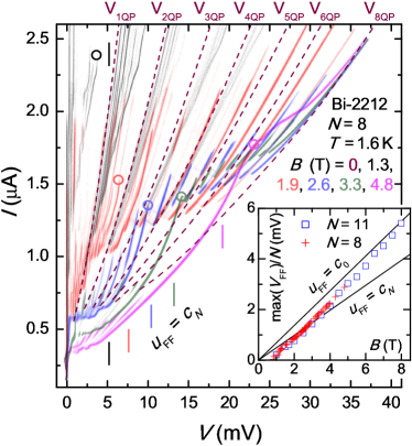
Figure 1: (Color online) $I$-$V$ characteristics of mesa 1 at different magnetic fields. Dashed lines represent quasiparticle branches at $B=0$. Development of flux-flow branches with increasing field is clearly seen. Circles mark maximum flux-flow voltages. Short lines indicate the velocity matching condition $u_{\mathrm{FF}}=c_{8}$. Inset: The maximum flux-flow voltage per junction vs. $B$ for mesa 1 ($N=8$) and mesa 2 ($N=11$). Lines correspond to flux-flow velocities equal to $c_{N}$ and $c_{0}$, respectively. It is seen that the experimentally observed flux-flow velocity becomes superluminal, $u_{\mathrm{FF}}>c_{N}$, at $B>2.6$T and approaches the Swihart velocity $c_{0}$ at high fields.

Unambiguous identification of the resonance modes $(m,n)$ requires first of all discrimination between individual (not phase-locked) and collective (phase-locked) Fiske steps. This is nontrivial, because, for instance, the voltage $1V_{m,1}$ of an individual in-phase step is close to the voltage $NV_{m,N}$ of a collective out-of-phase step, see Eqs. (4,5). Besides, not all junctions may participate in the collective resonance. For mesas with large $N>10$ different resonant modes $(m,n)$ form a very dense, almost continuous, Fiske step sequence. Therefore, bare analysis of voltage spacings is insufficient. To simplify discrimination between modes with different velocities, mesas with small $N$ should be analyzed. Below we mainly focus on mesa 1 with the smallest number of IJJs $N=8$.

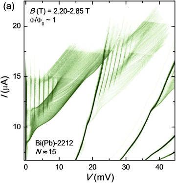
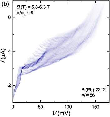
Figure 2: (Color online) $I$-$V$ oscillograms for continuous field sweeps around integer flux quanta per junction for Bi(Pb)-2212 mesas (a) 3 and (b) 4. At low fields in (a) both the continuously varying viscous flux-flow state and sharp, vertical, equidistant Fiske steps are simultaneously observed. At higher fields in (b) the whole flux-flow oscillogram is stratified into dense grids of resonances. This clearly demonstrates that the flux-flow $I$-$V$ characteristics in this case are not changing continuously with field, but switch between a variety of distinct resonant states.

Figure 3 shows $I$-$V$ oscillograms of mesa 1 in narrow field ranges corresponding to half-integer and integer number of flux quanta $\Phi/\Phi_{0}$ per IJJ. To check whether the observed Fiske steps are individual or collective, in the inset of Fig. 3(a) we compare steps at the first $V_{8\mathrm{FF}}$ flux-flow branch and the second $V_{7\mathrm{FF}}$ (with one junction in the QP state). To obtain $V_{7\mathrm{FF}}$, the first QP voltage $V_{1\mathrm{QP}}(B=0)$ is subtracted from the $V_{1\mathrm{QP}}+V_{7\mathrm{FF}}$ branch. Collective steps should decrease in proportion to the number of junctions, e.g., $7/8$ times. Individual steps, on the other hand, should maintain the same voltage at both flux-flow branches. This is the case at half-integer $\Phi/\Phi_{0}$ in Fig. 3(a) and (b). The dominant step at integer $\Phi/\Phi_{0}\simeq 3$, see Fig. 3(c), however, occurs at $8V_{1,8}$ at the $V_{8\mathrm{FF}}$ branch and at $7V_{1,8}$ at the next $V_{7\mathrm{FF}}$ branch, and is thus collective. Discrimination between individual and collective steps allows accurate identification of resonant modes $(m,n)$.

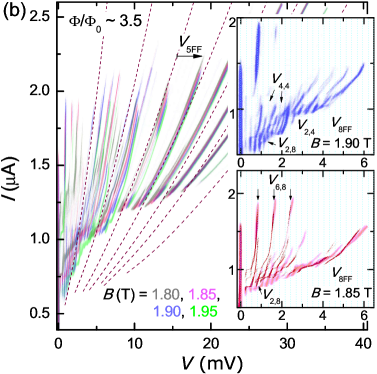
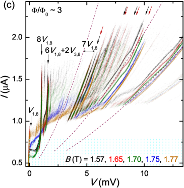
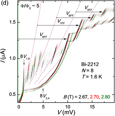
Figure 3: (Color online) $I$-$V$ oscillograms of mesa 1 (at constant $B$) in narrow field ranges near half-integer [(a) and (b)] and integer [(c) and (d)] $\Phi/\Phi_{0}$. A large variety of high-quality Fiske steps are seen. Also shown are the QP branches at $B=0$ (dashed lines). The grid-spacing is $V_{2,8}=0.27\,\mathrm{mV}$. The inset in (a) shows Fiske steps at the flux-flow branches with zero ($V_{8\mathrm{FF}}$) and one ($V_{7\mathrm{FF}}$) IJJ in the QP state, respectively. Voltage separation between steps is clearly independent of the number of junctions, showing that the Fiske steps here are from individual IJJs. The insets of panel (b) show the low bias region at $B=1.85\,\mathrm{T}$ and $1.90\,\mathrm{T}$. Several individual Fiske steps are marked. At integer $\Phi/\Phi_{0}$ in (c), by contrast, the prominent collective step $NV_{1,8}$ is seen, which scales with the number of junctions for $V_{8\mathrm{FF}}$ and $V_{7\mathrm{FF}}$. Two collective steps are also indicated in (d). Thus, IJJs behave more individually or collectively at half-integer or integer $\Phi/\Phi_{0}$, respectively.

The smallest step sequence $\simeq 0.135\,\mathrm{mV}$ is observed at integer $\Phi/\Phi_{0}$, see Fig. 3(c). It corresponds to the expected value $V_{1,8}$ for the lowest odd $m=1$ out-of-phase $n=8$ individual Fiske step. The corresponding slowest velocity $c_{8}\simeq 3.17\times 10^{5}\,\mathrm{m/s}$ is consistent with the estimation from Sec. II. Simultaneously, a strong collective Fiske step at $V=8V_{1,8}$ is observed, as marked in Figs. 3(c) and (d). It corresponds to the phase-locked state of the whole mesa at the same $(1,8)$ resonance. Steps with separation $2V_{1,8}$ are seen above the collective step in Fig. 3(c). They are due to switching between nearest odd $m=1$ and 3 out-of-phase $n=8$ resonances in individual IJJs, consistent with numerical simulations below.

At half-integer $\Phi/\Phi_{0}$ the smallest step sequence corresponds to the lowest even $m=2$ individual Fiske step $V_{2,8}\simeq 0.27\,\mathrm{mV}$, marked in Fig. 3(a) and insets of Fig. 3(b). The most prominent Fiske steps at half-integer $\Phi/\Phi_{0}$ correspond to individual even $m=4$ and $m=6$ out-of-phase resonances in Figs. 3(a) and 3(b), respectively, which are close to the velocity matching condition of Eq. (9).

While the Fiske step patterns vary significantly with magnetic field, they have certain common features for integer (more collective behavior, odd-$m$ modes) and half-integer (more individual behavior, even-$m$ modes) $\Phi/\Phi_{0}$. The step amplitudes oscillate strongly with $B$, with odd and even $m$ in anti-phase with each other, as expected. A complete overview of the modulation can be found in the supplementary.Supplem

$n$	1	2	3	4	5	6	7	8
$c_{n}\,({10^{5}\,\mathrm{m/s}})$	17.97	9.13	6.24	4.86	4.08	3.60	3.32	3.17
$c_{n}/c_{8}$	5.67	2.88	1.97	1.53	1.29	1.14	1.05	1.00
$V_{1,n}\,({\mathrm{mV}})$	0.765	0.389	0.266	0.207	0.174	0.153	0.141	0.135

Table 2: Calculated characteristic velocities $c_{n}$ for mesa 1, using $s=1.55\,\mathrm{nm}$, $\lambda_{ab}=200\,\mathrm{nm}$, and $t/\varepsilon_{\mathrm{r}}=0.112\,\mathrm{nm}$ and Eq. (1). Also given are the ratios $c_{n}/c_{8}$ and calculated Fiske step voltages $V_{1,n}=B_{0}sc_{n}/2$, where $B_{0}=0.55\,\mathrm{T}$ is the flux-quantization field.

IV.2 Superluminal resonances

So far, we discussed out-of-phase Fiske steps with voltages equal to multiple integers of $V_{1,8}$. Such steps, both individualFiskeInd and collective Fiske ; FiskeSlow , with similar velocities $c_{N}=2.5-3.5\times 10^{5}\,\mathrm{m/s}$ were observed previously, although with smaller relative amplitudes. However, in our case the full set of observed Fiske steps cannot be described solely by multiple integers of $V_{1,8}$. We can distinguish step sequences with different voltage spacings, which must correspond to resonances with higher velocities $c_{n}>c_{8}$, listed in Table 2.

In the flux flow region $V_{7\mathrm{FF}}$ of Fig. 3(c), where one IJJ has switched to the QP state, two sequences of steps with slightly different voltage spacings are seen at $1.57\,\mathrm{T}$ (black) and $1.65\,\mathrm{T}$ (red curve). Both step sequences start from the same $7V_{1,8}$ level, corresponding to the collective $(1,8)$ geometrical resonance in the remaining 7 IJJs. The lowest (black) step sequence has a step separation of $4V_{1,8}$ and is due to sequential switching of junctions from the lowest odd $m=1$ resonance $V_{1,8}$ to the odd resonance $V_{5,8}$ closest to the velocity matching condition at the same speed. The whole step sequence is then described by $V_{i}=(7-i)V_{1,8}+iV_{5,8}$, where $i=0,1,\,\ldots,7$ is the number of junctions in the $V_{5,8}$ state and the separation between steps is $V_{5,8}-V_{1,8}=4V_{1,8}$. The higher (red) step sequence also starts from the same $7V_{1,8}$ level, but the splitting between the two step sequences becomes progressively larger with increasing step number, as indicated by black and red arrows for steps number $3$ and $5$ in Fig. 3(c). This step sequence is described by a similar expression $V_{i}=(7-i)V_{1,8}+iV_{m,n}$, ($i=0,1,\,\ldots,7$). The corresponding eight (red) Fiske steps can be distinguished in Fig. 3(c). The involved resonance $V_{m,n}=1.05V_{5,8}$ is very close to $V_{5,7}$, which represents the first superluminal resonance $n=7$, see Table 2.

Individual step sequences

$$V_{i}=(N-i)V_{1,8}+iV_{m,n},\qquad({i=0,1,\,\ldots,N})$$

are observed at all integer $\Phi/\Phi_{0}$. At $\Phi/\Phi_{0}\simeq 5$ in Fig. 3(d), for example, nine steps can be distinguished on the $8V_{\mathrm{FF}}$ branch. At a first glance they may look similar to previously seen sub-branching due to onset of uncorrelated viscous flux-flow in individual IJJs.Bae2007 However, steps discussed here are resonant. In contrast to viscous flux-flow branches, which change monotonously with field, see Fig.2(a), these steps are periodically modulated in magnetic fieldSupplem and the step voltage is not changing continuously, but goes through discrete, although dense, set of values, see Fig. 2(b). This leads to the small splitting of steps in Fig. 3(c). Splitting of steps number $2$ – $4$ is also seen in Fig. 3(d). At certain conditions different step sequences can be observed at the same $B$, leading to a fine splitting as shown in the bottom inset of Fig. 3(b). The appearance of different step sequences is due to discrete, rather than continuous, change of the flux-flow voltage with $B$.

At $\Phi/\Phi_{0}\sim 2.5$, see Fig. 3(a), an individual step sequence with a voltage spacing of $0.42\,\mathrm{mV}$ is observed both in the flux-flow regions $V_{8\mathrm{FF}}$ and $V_{7\mathrm{FF}}$. The ratio of this voltage spacing to $V_{2,8}$ is $1.55$, which is close to the ratio expected for $c_{4}/c_{8}=1.53$, see Table 2. We, therefore, identify this voltage spacing with $V_{2,4}$. At the next half-integer $\Phi/\Phi_{0}\sim 3.5$ we observe two even-$m$ resonances for the same $n=4$ mode, $V_{2,4}$ and $V_{4,4}$, as indicated in the top inset of Fig. 3(b). In Fig. 3(d), an additional collective step is seen at $V\simeq 5\,\mathrm{mV}$ when the current is decreased from high bias. It may correspond to a phase-locked $8V_{3,4}$ Fiske step, or possibly $8V_{4,6}$.

IV.3 Fiske step modulation

The main panel in Fig. 4(a) shows Fraunhofer-like modulation of the critical current for mesa 1. Dashed vertical lines indicate the magnetic fields at integer $\Phi/\Phi_{0}$. Dominant and sub-dominant maxima of $I_{\mathrm{c}}(\Phi)$ at half-integer and integer $\Phi/\Phi_{0}$ correspond to rectangular and triangular fluxon lattices, respectively.Katterwe Fiske steps also modulate strongly with magnetic field, as shown in the lower inset of Fig. 4(a) for several prominent steps. It is expected that steps with even $m$ modulate in-phase with $I_{\mathrm{c}}(\Phi)$, i.e., have maxima at half-integer $\Phi/\Phi_{0}$. Steps with odd $m$ modulate out-of-phase with $I_{\mathrm{c}}(\Phi)$ and have maxima at integer $\Phi/\Phi_{0}$. Voltages of the chosen prominent Fiske steps are shown in the upper inset. Variation of the voltage demonstrates that switching between modes with different $m$ and $n$ occurs with variation of field.

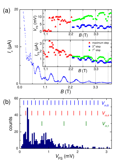
Figure 4: (Color online) (a) $I_{\mathrm{c}}(B)$ pattern for mesa 1. Grid lines corresponds to integer $\Phi/\Phi_{0}$. The lower inset shows modulation of amplitudes of some prominent Fiske steps. Triangles represent the Fiske steps with the highest amplitude at fields from $1\,\mathrm{T}$ to $2.25\,\mathrm{T}$. Squares and circles represent the $3^{\mathrm{rd}}$ resp. $7^{\mathrm{th}}$ step in individual Fiske step sequences at high bias at $B>2.3\,\mathrm{T}$ [as in Fig. 3(d) at $0.5\,\mathrm{\muup A}<I<1.5\,\mathrm{\muup A}$]. Voltages of the same steps are shown in the upper inset. (b) Probability histogram for observation of different steps separations in the field interval from 0 to $4\,\mathrm{T}$. Top vertical lines indicate out-of-phase Fiske steps, which are multiple integers of $V_{1,8}$. Apparently all observed steps cannot be described solely by out-of-phase resonances. Expected voltages for $n=4$ and $n=1$ superluminal steps are also indicated.

Figure 4(b) summarizes our main experimental results. It shows a probability histogram for all observed step voltage spacings in the field interval up to $B=4\,\mathrm{T}$. The step at $V_{2,8}\simeq 0.27\,\mathrm{mV}$ has the highest number of counts. However, vertical lines in the upper part of the figure indicate that all experimentally observed steps cannot be described solely by $(m,8)$ resonances. To explain the rich variety of steps, geometrical resonances with different velocities have to be present. Exact identification of all steps is rather complicated because velocity splitting creates rather dense and often overlapping voltage sequences even for $N=8$. Expected voltage positions for individual superluminal $n=4$ and $n=1$ Fiske steps are indicated in Fig. 4(b).

IV.4 The maximum flux-flow velocity

Since we have confidently identified the slowest velocity of light $c_{8}=3.17\times 10^{5}\,\mathrm{m/s}$, it is instructive to compare it with the maximum flux-flow velocity. In Fig. 1 voltages at the velocity matching condition $u_{\mathrm{FF}}=c_{8}$ and maximum flux-flow voltages are marked by short lines and circles, respectively. It is seen that the maximum flux-flow velocity is less, equal, and larger than $c_{8}$ for fields less, equal, and larger than $2.6\,\mathrm{T}$. Interestingly, nothing special happens with the flux-flow branch when it becomes superluminal, $u_{\mathrm{FF}}>c_{N}$. This is consistent with numerical simulationsFluxon and is due to the absence of Lorentz contraction of fluxons in strongly coupled, stacked Josephson junctions. The inset in Fig. 1 shows measured maximum flux-flow voltages per junction for mesas 1 and 2. The lines represent flux-flow voltages with velocities $c_{N}=3.17\times 10^{5}\,\mathrm{m/s}$ and $c_{0}=4.42\times 10^{5}\,\mathrm{m/s}$. Gradual increase of the maximum flux-flow velocity with field is clearly seen and is consistent with previous reports.Fiske ; Compar ; Cherenkov ; FFlowHatano ; FFLatyshev The maximum $u_{\mathrm{FF}}$ is approaching $c_{0}$ at high fields. A similar limiting velocity was obtained by numerical simulations for the case when fluxon stability is limited by Cherenkov radiation (see Fig. 7 in Ref. Fluxon, ).

V Numerical modelling

To get a better insight into experimental data, we performed numerical simulations of the coupled sine-Gordon equation with non-radiating boundary conditions (see Refs. [Fluxon, ; Modes, ] for details of the numerical procedure, analysis of Fiske steps with proper radiative boundary conditions can be found in Ref. [TheoryFiske, ]). To reproduce the real situation, we introduced a small gradient of $I_{\mathrm{c}}$ ($5\%$ per IJJ) from the top to the bottom of the mesa. We also considered the presence of the bulk crystal below the mesa and the additional top deteriorated junction.SecondOrder To model the crystal, we introduced an additional junction at the bottom of the stack with zero net bias current. The additional top junction was assumed to have a 100 times smaller $I_{\mathrm{c}}$. Passive top and bottom junctions do not cause any principle differences in fluxon dynamics. Although they may participate in geometrical resonances, they do not contribute to the flux-flow voltage. In simulations we used parameters of the mesa 1: $N=8$, $L=3.5\lambda_{\mathrm{J}}\simeq 2.4\,\mathrm{\muup m}$, and the damping coefficient $\alpha=0.01-0.05$. Small damping is important for excitation of a large variety of geometrical resonances. In order to reach various resonances the bias current was swept back and forth several times, mimicking experimental measurement.

Figure 5(a) and (b) show simulated $I$-$V$ curves (with subtracted top junction resistance) at $\Phi/\Phi_{0}=4.0$ for the case of uniform damping $\alpha_{i}=0.01$, $(i=1,2,...8)$. Panel (b) shows the total dc-voltage in a wide current range (current is normalized by the total QP resistance of the mesa). Basically all geometrical resonances with velocities from $c_{8}$ to $c_{1}$ are seen, consistent with previous simulations.FFlowSimul ; FFlowMachida

Panel (a) shows details of the subluminal flux-flow branch, $u_{\mathrm{FF}}<c_{8}$. Here also a large variety of Fiske steps is seen. The most frequent step separation is $V_{1,8}$ and $2V_{1,8}$ (the grid spacing). The largest collective step occurs at $8V_{7,8}$ close to the velocity matching condition, Eq. (9). However, a finer step structure with different voltages is developing in the top half of the flux-flow branch at $V>2.5\,\mathrm{mV}$. To understand its origin, in the inset we show individual voltages for all junctions. Vertical lines indicate positions of all possible Fiske steps $V_{m,n}$. The most prominent modes $(m,n)$ are indicated. As expected, in the considered case of integer $\Phi/\Phi_{0}$ only odd $m=1,3,5,7$ resonances are excited. The observed even $2V_{1,8}$ step separation is due to sequential switching between nearest odd-$m$ steps, as discussed in connection with Fig. 3(c). However, not all steps in the subluminal regime are due to out-of-phase $n=8$ resonances. Several superluminal resonances, $n=3,4,5,6$, are also excited.

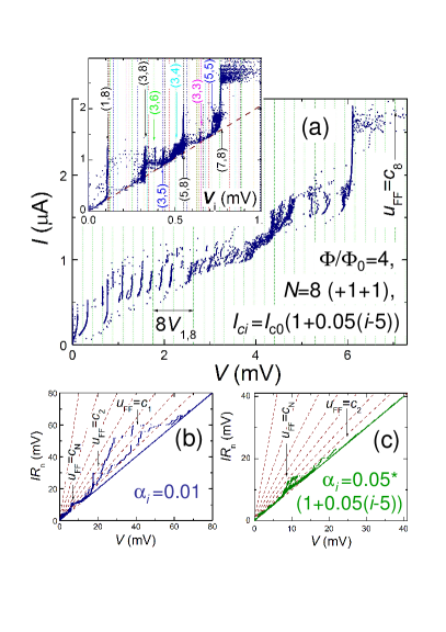
Figure 5: (Color online) Simulated $I$-$V$ characteristics at $\Phi/\Phi_{0}=4.0$ for a mesa with $N=8$ active IJJs and two passive junctions at the top and bottom of the mesa. Panels (a) and (b) represent simulations for a small nonuniformity of the critical current ($5\%$ per IJJ) and uniform damping parameter $\alpha_{i}=0.01$. (a) The subluminal $u_{\mathrm{FF}}<c_{8}$ part of the flux-flow characteristics. Inset shows $I-V$ characteristics of individual junctions. Vertical lines show positions of all possible Fiske steps. Appearance of various superluminal resonances is indicated. (b) The $I-V$ in a wider range. Dashed lines represent QP branches. Very strong superluminal Fiske steps are seen. Panel (c) shows the $I-V$ characteristics of a mesa with nonuniform $I_{ci}$ and $\alpha_{i}\simeq 0.05$, both increase by $5\%$ per IJJ from the top to the bottom of the mesa. It is seen that variation of junction resistances strongly suppresses high-frequency resonances.

Our simulations demonstrate that superluminal resonances $c_{n}>c_{N}$ can be excited by subluminal flux-flow $u_{\mathrm{FF}}<c_{N}$, which is in agreement with experimental data reported above. Although such possibility was not discussed before, it is probably not surprising because qualitatively the same happens with out-of-phase resonances. The necessary condition is given by Eq. (8), which clearly allows excitation of superluminal modes $n<N$ at $u_{\mathrm{FF}}<c_{N}$. For example, in the considered case $N=8$, the first fastest $(1,1)$ mode can be excited at $u_{\mathrm{FF}}\simeq c_{8}$, provided $\Phi/\Phi_{0}>c_{1}/2c_{8}\simeq 3$.

V.1 Quality factors of different modes

The quality factor $Q=\omega RC$ is an important characteristic of the resonance. Here, $R$ is the effective damping resistance and $C$ the capacitance of the junction. High-quality geometrical resonances are crucial for realization of coherent FFOs:TheoryFiske

1. They amplify the emission power $P\propto E_{\mathrm{ac}}^{2}\propto Q^{2}$. This is especially important for stacked FFOs since there is no Lorentz contraction of the fluxon at the velocity matching condition,Fluxon which is used for amplification of the electric field in a single junction FFO.Koshelets

2. They reduce the radiation linewidth of the FFO $\propto 1/Q$.

3. They may impose their order on the fluxon lattice even at subluminal flux-flow velocities, as follows from numerical simulations in Fig. 5(a). In particular, in-phase resonances may stabilize the rectangular fluxon lattice, facilitating coherent amplification of radiation $P\propto Q^{2}N^{2}$. The forced transformation of the fluxon lattice occurs when the resonant standing wave electric field $E_{\mathrm{ac}}\propto 1/Q$ is larger than the fields of the fluxons. Therefore, high $Q$ is critical for such forced transformation.

Although numerical simulations presented above describe well the subluminal $u_{\mathrm{FF}}<c_{8}$ part of experimental flux-flow branches [cf. Fig. 5(a) and Fig. 3], there is a clear discrepancy in the superluminal regime. Numerical simulationsFFlowSimul ; FFlowMachida predict very strong superluminal Fiske steps, which have even larger amplitudes than the out-of-phase steps at $u_{\mathrm{FF}}\leq c_{8}$, as seen from Fig. 5(b). In those simulations larger $Q$ for higher Fiske steps is simply the consequence of linear growth of $Q\propto\omega$ for constant $R$ and $C$. To clarify this discrepancy we consider the quality factors of different modes $(m,n)$,

$$Q_{m,n}=\frac{\pi c_{n}mR(\omega)C}{L}.$$ (10)

Here $L$ is the junction length. There are two counteracting contributions. On the one hand, $Q\propto\omega_{m,n}$ and should be larger for high speed and large $m$ modes. On the other hand, the effective resistance $R(\omega)$ is decreasing with increasing frequency. For single Josephson junctions it is very well established that at high frequencies $R(\omega)$ is approaching the radiative resistance of the circuitry $R_{\mathrm{rad}}\sim 50\,\Omega$Martinis due to predominance of radiative losses into outer-space.

As emphasized in Ref. [TheoryFiske, ], in stacked junctions $R(\omega)$ strongly depends on $n$. Out-of-phase modes interfere destructively, cancelling radiative losses. Therefore, $Q$ of those non-emitting modes is determined by the large QP resistance $R_{\mathrm{QP}}$:

$$Q_{m,N}=\frac{\pi c_{N}mR_{\mathrm{QP}}C}{L}.$$ (11)

Taking parameters for our mesa 1, $c_{N}\simeq 3.17\times 10^{5}\,\mathrm{m/s}$, $R_{\mathrm{QP}}\simeq 2\,\mathrm{k\Omega}$ at $T=1.6\,\mathrm{K}$, intrinsic capacitance $C\simeq 70\,\mathrm{fF/\muup m^{2}}$, $L=2.7\,\mathrm{\muup m}$, $L_{y}=1.4\,\mathrm{\muup m}$, and $m=2$ we obtain $Q_{2,8}\simeq 390$. This very large value is consistent with the sharp, large amplitude $(2,8)$ steps seen in Fig. 3(a). It is also consistent with observation of out-of-phase Fiske steps in much longer junctions $L=50\,\mathrm{\muup m}$.Fiske The same is true for other destructively interfering, non-radiative modes

$$n^{*}=N-2i,\qquad i=0,1,2,\ldots,\mathrm{int}\left[(N-1)/2\right].$$ (12)

For the in-phase mode electric fields from all junctions interfere constructively resulting in large coherent emission. In this case $R$ is determined by radiative losses,

$$Q_{m,1}=\frac{\pi c_{1}mR_{\mathrm{rad}}C}{L}.$$ (13)

Using parameters of mesa 1, $c_{1}\simeq 1.8\times 10^{6}\,\mathrm{m/s}$, and assuming $R_{\mathrm{rad}}=50\,\mathrm{\Omega}$ we obtain $Q_{2,1}\simeq 46$. Thus, radiative geometric resonances should have substantially smaller $Q$ than the non-radiative ones.TheoryFiske

For mesa 1 with $N=8$ all even-$n$ modes are non-radiative, Eq. (12). Fiske steps due to such resonances should have the highest $Q$ and amplitude. This is consistent with our observation that even-$n$ modes correspond to the most prominent Fiske steps, see Fig. 3. Similarly, more smeared, high-voltage Fiske steps at larger fields could indicate enhanced emission and radiative losses from the radiative superluminal resonances. The asymmetry between even and odd $n$ Fiske steps is an indirect evidence for significant coherent radiation emission from the stack.TheoryFiske

V.2 Suppression of superluminal resonances by the spread in junction resistances.

Collective, high-voltage Fiske steps can also be suppressed by another trivial reason: due to the spread in junction resistances $\Delta R$. Indeed, if junctions in the stack have slightly different QP resistances $R_{i}$, the Fiske step $V_{m,n}$ would occur at different currents $I_{i}=V_{m,n}/R_{i}$. Therefore, the collective Fiske step could be observed only if the amplitude of the steps $\Delta I>(V_{m,n}/R_{i}^{2})\Delta R$. Apparently, this condition is more difficult to satisfy for high voltage and low $Q$ resonances.

To demonstrate this, in Fig. 5(c) we present numerical simulations for nonuniform damping $\alpha_{i}\simeq 0.05$, increasing by $5\%$ per IJJ from the top to the bottom of the mesa and with the corresponding spread in the QP resistances $R_{i}\propto 1/\alpha_{i}$. The rest of the parameters are similar to that in panels (a) and (b). From comparison with panel (b) it is clear that the amplitude of low frequency out-of-phase $c_{N}$ steps $IR_{n}\simeq 10$ mV is unchanged, but all high frequency superluminal resonances are strongly reduced. The fastest in-phase resonances are practically nonexisting. We emphasize that in the considered case this is not due to radiative losses, but is caused by the trivial reason that junctions can not be synchronized because it is impossible to keep them at the same voltage for a given current. Note that the spread in $I_{c}$ is not preventing the synchronization and is, therefore, much less detrimental for resonances, as seen from Fig. 5(b). In practice, both low $Q$ due to radiative lossesTheoryFiske and enhanced sensitivity to resistance spread may explain the abundance of the highest speed Fiske steps in experiment.

Conclusions

In conclusion, careful alignment of magnetic field allowed observation of a large variety of Fiske steps in small Bi-2212 mesas. Small number of IJJs in the mesa allowed accurate identification of different resonant modes. Different resonance modes, including superluminal with velocities larger than the lowest velocity of electromagnetic waves $c_{N}$, were observed. It was shown both experimentally and theoretically that superluminal geometrical resonances can be excited in the subluminal flux-flow state. Superluminal flux-flow state with the maximum flux-flow velocity up to the Swihart velocity $c_{0}\simeq 1.4c_{N}$ was also reported. The most prominent observed Fiske steps correspond to non-emitting resonance modes $n^{*}$, Eq. (12). The corresponding asymmetry between even and odd-$n$ resonances can be viewed as indirect evidence for significant coherent emission from intrinsic Josephson junctions.TheoryFiske

- (1) A. Laub, T. Doderer, S. G. Lachenmann, R. P. Huebener and V. A. Oboznov, Phys. Rev. Lett. 75, 1372 (1995).
- (2) V. M. Krasnov, Phys. Rev. B 63, 064519 (2001). Note the reverse numeration of the modes there: is the slowest and is the fastest mode.
- (3) S. Sakai, A. V. Ustinov, H. Kohlstedt, A. Petraglia, and N. F. Pedersen, Phys. Rev. B 50, 12905 (1994).
- (4) S. Sakai, A. V. Ustinov, N. Thyssen, and H. Kohlstedt, Phys. Rev. B 58, 5777 (1998).
- (5) R. Kleiner, Phys. Rev. B 50, 6919 (1994).
- (6) G. Hechtfischer, R. Kleiner, A. V. Ustinov, and P. Müller, Phys. Rev. Lett. 79, 1365 (1997).
- (7) S. Savel’ev, V. A. Yampol’skii, A. V. Rakhmanov, and F. Nori, Rep. Prog. Phys. 73, 026501 (2010).
- (8) V. M. Krasnov and D. Winkler, Phys. Rev. B 56, 9106 (1997).
- (9) P. Barbara, A. B. Cawthorne, S. V. Shitov, and C. J. Lobb, Phys. Rev. Lett. 82, 1963 (1999).
- (10) S. V. Shitov, A. V. Ustinov, N. Iosad, and H. Kohlstedt, J. Appl. Phys. 80, 7134 (1996).
- (11) V. M. Krasnov, Phys. Rev. B 79, 214510 (2009).
- (12) I. E. Batov, X. Y. Jin, S. V. Shitov, Y. Koval, P. Müller, and A. V. Ustinov, Appl. Phys. Lett. 88, 262504 (2006).
- (13) L. Ozyuzer, A. E. Koshelev, C. Kurter, N. Gopalsami, Q. Li, M. Tachiki, K. Kadowaki, T. Yamamoto, H. Minami, H. Yamaguchi, T. Tachiki, K. E. Gray, W. K. Kwok, and U. Welp, Science 318, 1291 (2007).
- (14) M. H. Bae, H. J. Lee, and J. H. Choi, Phys. Rev. Lett. 98, 027002 (2007).
- (15) R. Kleiner, T. Gaber, and G. Hechtfischer, Physica C 362, 29 (2001).
- (16) M. Machida, T. Koyama, A. Tanaka, and M. Tachiki, Physica C 330, 85 (2000).
- (17) A. E. Koshelev and I. S. Aranson, Phys. Rev. Lett. 85, 3938 (2000).
- (18) D. A. Ryndyk, V. I. Pozdnjakova, I. A. Shereshevskii and N. K. Vdovicheva, Phys. Rev. B 64, 052508 (2001).
- (19) V. M. Krasnov, Phys. Rev. Lett. 103, 227002 (2009); ibid., 97, 257003 (2006).
- (20) L. N. Bulaevskii and A. E. Koshelev, Phys. Rev. Lett. 99, 057002 (2007).
- (21) X.Hu and S. Z. Lin, Supercond. Sci.Technol. 23, 053001 (2010).
- (22) T. Tachiki and T. Uchida, J. Appl. Phys. 107, 103920 (2010).
- (23) M. Tachiki, S. Fukuya, and T. Koyama, Phys. Rev. Lett. 102, 127002 (2009).
- (24) K. Kadowaki, M. Tsujimoto, K. Yamaki, T. Yamamoto, T. Kashiwagi, H. Minami, M. Tachiki, and R.A. Klemm, J. Phys. Soc. Japan 79, 023703 (2010).
- (25) V. M. Krasnov, arXiv:1005.2963 [cond-mat.supr-con] (unpublished).
- (26) V. P. Koshelets and S. V. Shitov, Supercond. Sci. Technol. 13, R53 (2000).
- (27) S. O. Katterwe and V. M. Krasnov, Phys. Rev. B 80, 020502(R) (2009).
- (28) V. M. Krasnov, V. A. Oboznov, V. V. Ryazanov, N. Mros, A. Yurgens, and D. Winkler, Phys. Rev. B 61, 766 (2000).
- (29) Partial Lorentz contraction of the fluxon at occurs only in double stacked junctions, see e.g. V. M. Krasnov and D. Winkler, Phys. Rev. B 60, 13179 (1999); V. M. Krasnov, Phys. Rev. B 60, 9313 (1999).
- (30) V. M. Krasnov, N. Mros, A. Yurgens, and D. Winkler, Phys. Rev. B 59, 8463 (1999).
- (31) S. M. Kim, H. B. Wang, T. Hatano, S. Urayama, S. Kawakami, M. Nagao, Y. Takano, T. Yamashita, and K. Lee, Phys. Rev. B 72, 140504(R) (2005).
- (32) Y. I. Latyshev, A. E. Koshelev, V. N. Pavlenko, M. B. Gaifullin, T. Yamashita, and Y. Matsuda, Physica C 367, 365 (2002).
- (33) Y. D. Jin, H. J. Lee, A. E. Koshelev, G. H. Lee, and M. H. Bae, Europhys. Lett. 88, 27007 (2009).
- (34) M. H. Bae, J. H. Choi, and H. J. Lee, Phys. Rev. B 75, 214502 (2007).
- (35) S. J. Kim, T. Hatano, and M. Blamire, J. Appl. Phys. 103, 07C716 (2008).
- (36) A. L. Fetter, and M. J. Stephen, Phys. Rev. 168, 475 (1968).
- (37) I. O. Kulik, JETP Lett. 2, 84 (1965).
- (38) I. M. Dmitrenko, I. K. Yanson, and V. M. Svistunov, JETP Lett. 2, 10 (1965); M. Cirillo, N. Gronbech-Jensen, M. R. Samuelsen, M. Salerno and G. V. Rinati, Phys. Rev. B 58, 12377 (1998).
- (39) V. M. Krasnov, Phys. Rev. B 65, 140504 (2002).
- (40) V. M. Krasnov, T. Bauch, and P. Delsing, Phys. Rev. B 72, 012512 (2005).
- (41) A. Irie, S. Kaneko, and G. I. Oya, Int. J. Mod. Phys. 13, 3678 (1999).
- (42) Magnetic field modulation of Fiske steps and the critical current can seen in the accompanying animation : see EPAPS Document No…
- (43) H. B. Wang, S. Urayama, S. M. Kim, S. Arisawa, T.Hatano, and B.Y. Zhu, Appl. Phys. Lett. 89, 252506 (2006).
- (44) J. M. Martinis, M. H. Devoret and J. Clarke, Phys. Rev. B 35, 4682 (1987).