Controlling Molecular Scattering by Laser-Induced Field-Free Alignment

Abstract

We consider deflection of polarizable molecules by inhomogeneous optical fields, and analyze the role of molecular orientation and rotation in the scattering process. It is shown that molecular rotation induces spectacular rainbow-like features in the distribution of the scattering angle. Moreover, by preshaping molecular angular distribution with the help of short and strong femtosecond laser pulses, one may efficiently control the scattering process, manipulate the average deflection angle and its distribution, and reduce substantially the angular dispersion of the deflected molecules. We provide quantum and classical treatment of the deflection process. The effects of strong deflecting field on the scattering of rotating molecules are considered by the means of the adiabatic invariants formalism. This new control scheme opens new ways for many applications involving molecular focusing, guiding and trapping by optical and static fields.

I Introduction

Optical dipole forces acting on molecules in nonresonant laser fields is a hot subject of many recent experimental studies Deflection_general ; Lens ; Prism ; Barker-new . By controlling molecular translational degrees of freedom with laser fields Friedrich ; Seideman ; Friedrich1 ; Gordon ; Fulton ; Fulton1 , novel elements of molecular optics can be realized, including molecular lens Deflection_general ; Lens and molecular prism Prism . The mechanism of molecular interaction with a nonuniform laser field is rather clear: the field induces molecular polarization, interacts with it, and deflects the molecules along the intensity gradient. As most molecules have anisotropic polarizability, the deflecting force depends on the molecular orientation with respect to the deflecting field. Previous studies on optical molecular deflection have mostly considered randomly oriented molecules, for which the deflection angle is somehow dispersed around the mean value determined by the orientation-averaged polarizability. The latter becomes intensity-dependent for strong enough fields due to the field-induced modification of the molecular angular motion Zon ; Friedrich . This adds a new ingredient for controlling molecular trajectories Friedrich ; Seideman ; Friedrich1 ; Gordon ; Barker-new , which is important, but somehow limited because of using the same fields for the deflection process and orientation control.

In this work, we show that the deflection process can be significantly affected and controlled by preshaping molecular angular distribution before the molecules enter the interaction zone. This can be done with the help of numerous recent techniques for laser molecular alignment, which use single or multiple short laser pulses (transform-limited, or shaped) to align molecular axes along certain directions. Short laser pulses excite rotational wavepackets, which results in a considerable transient molecular alignment after the laser pulse is over, i.e. at field-free conditions (for reviews on field-free alignment, see, e.g. Stapelfeldt ; Stapelfeldt1 ). Field-free alignment was observed both for small diatomic molecules as well as for more complex molecules, for which full three-dimensional control was realized 3D1 ; 3D2 ; 3D3 .

We demonstrate that the average scattering angle of the deflected molecules and its distribution may be dramatically modified by a proper field-free prealignment. By separating the processes of the angular shaping and the actual deflection, one gets a flexible tool for tailoring molecular motion in inhomogeneous optical and static fields.

The main principles of this new approach were briefly introduced in our recent Letter ourPRL . Here we present a much more elaborated analysis of the control mechanisms, including also a detailed comparison between the quantum and classical aspects of the problem, and discussion of the strong field effects in molecular scattering.

In Sec. II we present the deflection scheme, as well as heuristic classical discussion on the anticipated role of molecular rotation on the deflection process (both for thermal and prealigned molecules). In Sec III we verify these predictions by the means of the quantum treatment of the problem in the limit of the relatively weak deflecting field (that does not disturb significantly the rotational motion). The strength of the prealigning field is not restricted here. Full classical treatment of the molecular deflection at such conditions (including thermal effects) is given in Sec. IV, where we find a good correspondence between the classical and quantum calculations. Motivated by this agreement, we provide in Sec. V a full classical analysis of the molecular scattering by strong deflecting field using the adiabatic invariants formalism. Finally we summarize our results in Sec. VI.

II Deflection of field-free aligned molecules

Although our arguments are rather general, we follow for certainty a deflection scheme that brings to mind the experiment by Stapelfeldt $et$ $al$ Deflection_general who used a strong IR laser to deflect a $CS_{2}$ molecular beam, and then addressed a portion of the deflected molecules (at a preselected place and time) by an additional short and narrow ionizing pulse. Consider deflection (in $z$ direction) of a linear molecule moving in $x$ direction with velocity $v_{x}$ and interacting with a focused nonresonant laser beam that propagates along the $y$ axis (Fig. 1).

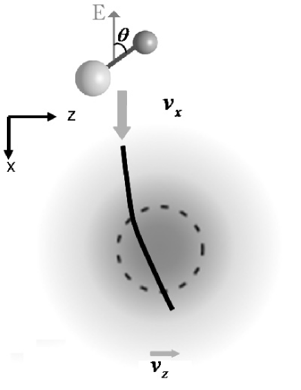
Figure 1: The deflection scheme. A polarized (in the $z$ direction) laser field propagates toward the plane of the paper ($y$ direction). The linear molecules, initially moving along the $x$ direction (with velocity $v_{x}$), are deflected by the potential gradient (deflection velocity $v_{z}$).

The spatial profile of the laser electric field in the $xz$-plane is:

$$E=E_{0}\exp[-(x^{2}+z^{2})/\omega_{0}^{2}]\exp[-2\ln 2t^{2}/\tau^{2}].$$ (1)

The interaction potential of a linear molecule in the laser field is given by:

$$U=-\frac{1}{4}E^{2}\left(\alpha_{\parallel}\cos^{2}\theta+\alpha_{\perp}\sin^{2}\theta\right),$$ (2)

where $E$ is defined in Eq. 1, and $\alpha_{\parallel}$ and $\alpha_{\perp}$ are the components of the molecular polarizability along the molecular axis, and perpendicular to it, respectively. Here $\theta$ is the angle between the electric field polarization direction (along the laboratory $z$ axis) and the molecular axis. A molecule initially moving along the $x$ direction will acquire a velocity component $v_{z}$ along $z$-direction. We consider the perturbation regime corresponding to a small deflection angle, $\gamma\thickapprox v_{z}/v_{x}$. We substitute $x=v_{x}t$, and consider $z$ as a fixed impact parameter. The deflection velocity is given by:

$$v_{z}=\frac{1}{M}\int_{-\infty}^{\infty}F_{z}dt=-\frac{1}{M}\int_{-\infty}^{\infty}\left(\overrightarrow{\nabla}U\right)_{z}dt.$$ (3)

Here $M$ is the mass of the molecules, and $F_{z}$ is the deflecting force. The time-dependence of the force $F_{z}$ (and potential $U$) in Eq.(3) comes from three sources: pulse envelope, projectile motion of the molecule through the laser focal area, and time variation of the angle $\theta$ due to molecular rotation. For simplicity, we start with the case of the relatively weak deflecting field that does not affect significantly the rotational motion. Such approximation is justified, say for $CS_{2}$ molecules with the rotational temperature $T=5K$, which are subject to the deflecting field of $3\cdot 10^{9}W/cm^{2}$. The corresponding alignment potential $U\approx-\frac{1}{4}\left(\alpha_{\parallel}-\alpha_{\perp}\right)E_{0}^{2}\approx 0.04\ meV$ is an order of magnitude smaller than the thermal energy $k_{B}T$, where $k_{B}$ is Boltzmann’s constant. This assumption is even more valid if the molecules were additionally subject to the aligning pulses prior to deflection. The case of a strong deflecting field will be considered later in Sec.V.

Since the rotational time scale is the shortest one in the problem, we average the force over the fast rotation, and arrive at the following expression for the deflection angle, $\gamma=v_{z}/v_{x}$:

$$\gamma=\gamma_{0}\ \left[\alpha_{||}{\cal A}+\alpha_{\bot}(1-{\cal A})\right]/\overline{\alpha}$$ (4)

Here $\overline{\alpha}=1/3\alpha_{||}+2/3\alpha_{\bot}$ is the orientation-averaged molecular polarizability, and ${\cal A}=\overline{\cos^{2}\theta}$ denotes the time-averaged value of $\cos^{2}\theta$. This quantity depends on the relative orientation of the vector of angular momentum and the polarization of the deflecting field. It is different for different molecules of the incident ensemble, which leads to the randomization of the deflection process. The constant $\gamma_{0}$ presents the average deflection angle for an isotropic molecular ensemble:

$$\gamma_{0} = \frac{\overline{\alpha}E_{0}^{2}}{4Mv_{x}^{2}}\left(\frac{-4z}{\omega_{0}}\right)$$ (5)

$$\times \sqrt{\frac{\pi}{2}}\left(1+\frac{2\omega_{0}^{2}\ln 2}{\tau^{2}v_{x}^{2}}\right)^{-1/2}\exp\left(-\frac{2z^{2}}{\omega_{0}^{2}}\right)$$

We provide below some heuristic classical arguments on the anticipated statistical properties of ${\cal A}$ and $\gamma$ (both for thermal and prealigned molecules).

Consider a linear molecule that rotates freely in a plane that is perpendicular to the vector $\overrightarrow{J}$ of the angular momentum (see Fig.(2)).

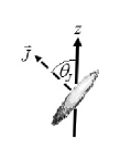
Figure 2: A molecule rotates with the angular momentum $\vec{J}$ forming an angle $\theta_{J}$ with the laboratory $z$ axis.

The projection of the molecular axis on the vertical $z$-direction is given by:

$$\cos\theta(t)=\cos(\omega t)\sin\theta_{J},$$ (6)

where $\theta_{J}$ is the angle between $\vec{J}$ and $z$-axis, and $\omega$ is the angular frequency of molecular rotation. Averaging over time, one arrives at:

$${\cal A}=\overline{\cos^{2}\theta}=\frac{1}{2}\sin^{2}\theta_{J}.$$ (7)

In a thermal ensemble, vector $\vec{J}$ is randomly oriented in space, with isotropic angular distribution density $1/2\sin(\theta_{J})$. The mean value of the deflection angle is $\langle\gamma\rangle=\gamma_{0}$. Eq.(7) allows us to obtain the distribution function, $f({\cal A})$ for ${\cal A}$ (and the related deflection angle) from the known isotropic distribution for $\theta_{J}$. Since the inverse function $\theta_{J}({\cal A})$ is multivalued, one obtains

$$f({\cal A})=\sum_{i=1}^{2}\frac{1}{2}\sin\theta_{J}^{(i)}{\left|\frac{d{\cal A}}{d\theta_{J}^{(i)}}\right|}^{-1}=\frac{1}{\sqrt{1-2{\cal A}}},$$ (8)

where we summed over the two branches of $\theta_{J}({\cal A})$. This formula predicts an unimodal rainbow singularity in the distribution of the scattering angles at the maximal value $\gamma=\gamma_{0}(\alpha_{||}+\alpha_{\bot})/2\overline{\alpha}$  (for ${\cal A}=1/2$), and a flat step near the minimal one $\gamma=\gamma_{0}\alpha_{\bot}/\overline{\alpha}$  (for ${\cal A}=0$).

Assume now that the molecules are prealigned before entering the deflection zone by a strong and short laser pulse that is polarized perpendicular to the polarization direction of the deflecting field (e.g., in $x$-direction). Such a pulse forces the molecules to rotate preferentially in the planes containing the $x$-axis. As a result, the vector $\vec{J}$ of the angular momentum is confined to the $yz$-plane, and angle $\theta_{J}$ becomes uniformly distributed in the interval $[0,\pi]$ with probability density $1/\pi$. The corresponding probability distribution for ${\cal A}$ takes the form

$$f({\cal A})=\frac{\sqrt{2}}{\pi}\frac{1}{\sqrt{{{\cal A}(1-2{\cal A}})}}$$ (9)

In contrast to Eq.(8), Eq.(9) suggests a bimodal rainbow in the distribution of deflection angles, with singularities both at the minimal and the maximal angles. Finally, we proceed to the most interesting case when the molecules are prealigned by a short strong laser pulse that is polarized parallel to the direction of the deflecting field. After excitation by such a pulse, the vector of the angular momentum of the molecules is preferentially confined to the $xy$-plane, and the angle $\theta_{J}$ takes a well defined value of $\theta_{J}\approx\pi/2$ which corresponds to ${\cal A}=1/2$. In this way, the molecules experience the maximally possible time-averaged deflecting force which is the same for all the particles of the ensemble. As a result, the dispersion of the scattering angles is reduced dramatically. The distribution of the deflection angle $\gamma$ transforms to a narrow peak (asymptotically - a $\delta$-function) near the maximal value, $\gamma=\gamma_{0}(\alpha_{||}+\alpha_{\bot})/2\overline{\alpha}$.

III Quantum Treatment

For a more quantitative treatment, involving analysis of the relative role of the quantum and thermal effects on one hand, and the strength of the prealigning pulses on the other hand, we consider quantum-mechanically the deflection of a linear molecule described by the Hamiltonian:

$${\cal H}=\hat{J}^{2}/(2I).$$ (10)

Here $\hat{J}$ is operator of angular momentum, and $I$ is the moment of inertia, which is related to the molecular rotational constant, $B=\hbar/(4\pi Ic)$ ($c$ is speed of light). Assuming again that the deflecting field is too weak to modify molecular alignment, we consider scattering in different $|J,m\rangle$ states independently. The deflection angle is given by Eq.(4), in which ${\cal A}$ is replaced by

$${\cal A}_{J,m}=\langle J,m|\cos^{2}\theta|J,m\rangle=\frac{1}{3}+\frac{2}{3}\frac{J(J+1)-3m^{2}}{(2J+3)(2J-1)}.$$ (11)

In the quantum case, the continuous distribution of the angles $\gamma$ is replaced by a set of discrete lines, each of them weighted by the population of the state $|J,m\rangle$. Fig. 3 shows the distribution of ${\cal A}_{J,m}$ in the thermal case for various values of the dimensionless parameter $J_{T}=\sqrt{k_{B}T/(hBc)}$ that represents the typical ”thermal” value of $J$ (for $J_{T}\geq 1$). For $CS_{2}$ molecules, the values of $J_{T}=5,15$ correspond to $T=3.9K$ and $T=35K$, respectively.

Figure 3: Quantum distribution of ${\cal A}_{J,m}$ in the thermal case. Panels (a) and (b) correspond to $J_{T}=5$ and $J_{T}=15$, respectively. Histogram in panel (c) shows a coarse-grained version of the distribution in panel (b).

The distribution of discrete values of ${\cal A}_{J,m}$ demonstrates a non-trivial pattern. In particular, the values exceeding the classical limit $0.5$ correspond to the states $|J,m=0\rangle$ (see Eq.(11)), and they rapidly approach that limit as $J$ grows. After the coarse-grained averaging, however, the distribution shows the expected unimodal rainbow feature (see Eq.(8)) for large enough $J_{T}$.

If the molecules are subject to a strong femtosecond prealigning pulse, the corresponding interaction potential is given by Eq. (2), in which $E$ is replaced by the envelope $\epsilon$ of the femtosecond pulse. If the pulse is short compared to the typical periods of molecular rotation, it may be considered as a delta-pulse. In the impulsive approximation, one obtains the following relation between the angular wavefunction before and after the pulse applied at $t=0$ (see e.g. Gershnabel , and references therein):

$$\Psi(t=0^{+})=\exp(iP\cos^{2}\theta)\Psi(t=0^{-}),$$ (12)

where the kick strength, $P$ is given by:

$$P=\left(1/4\hbar\right)\cdot(\alpha_{||}-\alpha_{\bot})\int_{-\infty}^{\infty}\epsilon^{2}(t)dt.$$ (13)

Here we assumed the vertical polarization (along $z$-axis) of the pulse. Physically, the dimensionless kick strength, $P$ equals to the typical amount of angular momentum (in the units of $\hbar$) supplied by the pulse to the molecule. For example, in the case of $CS_{2}$ molecules, the values of $P=5,25$ correspond to the excitation by $0.5ps$ (FWHM) laser pulses with the maximal intensity of $4.6\cdot 10^{11}W/cm^{2}$ and $2.3\cdot 10^{12}W/cm^{2}$, respectively. For the vertical polarization of the laser field, $m$ is a conserved quantum number. This allows us to consider the excitation of the states with different initial $m$ values separately. In order to find $\Psi(t=0^{+})$ for any initial state, we introduce an artificial parameter $\xi$ that will be assigned the value $\xi=1$ at the end of the calculations, and define

$$\Psi_{\xi}=\exp\left[(iP\cos^{2}\theta)\xi\right]\Psi(t=0^{-})=\sum_{J}c_{J}(\xi)|J,m\rangle.$$ (14)

By differentiating both sides of Eq.(14) with respect to $\xi$, we obtain the following set of differential equations for the coefficients $c_{J}$:

$$\dot{c}_{J^{\prime}}=iP\sum_{J}c_{J}\langle J^{\prime},m|\cos^{2}\theta|J,m\rangle,$$ (15)

where $\dot{c}=dc/d\xi$. The diagonal matrix elements in Eq.(15) are given by Eq.(11), the off-diagonal ones can be found using recurrence relations for the spherical harmonics Arfken . Since $\Psi_{\xi=0}=\Psi(t=0^{-})$ and $\Psi_{\xi=1}=\Psi(t=0^{+})$ (see Eq.(14)), we solve numerically this set of equations from $\xi=0$ to $\xi=1$, and find $\Psi(t=0^{+})$. In order to consider the effect of the field-free alignment at thermal conditions, we repeated this procedure for every initial $|J_{0},m_{0}\rangle$ state. To find the modified population of the $|J,m\rangle$ states, the corresponding contributions from different initial states were summed together weighted with the Boltzmann’s statistical factors:

$$f({\cal A}_{J,m_{0}}) = \sum_{J_{0},\bar{J}}\frac{\exp(-E^{J_{0}}/K_{B}T)}{Q_{rot}}$$ (16)

$$\times |c_{\bar{J}}|^{2}\delta({\cal A}_{J,m_{0}},{\cal A}_{\bar{J},m_{0}}),$$

where $c_{J}$ are the coefficients (from Eq. 15) of the wave packet that was excited from the initial state $|J_{0},m_{0}\rangle$; $\delta$ is the Kronecker delta, and $Q_{rot}$ is the rotational partition function. It worth mentioning that different combinations of $J$ and $m$ may correspond to the same value of ${\cal A}_{J,m}$, which necessitates the presence of the Kronecker delta in Eq. (16). For symmetric molecules, statistical spin factor should be taken into account. For example, for $CS_{2}$ molecules in the ground electronic and vibrational state, only even $J$ values are allowed due to the permutation symmetry for the exchange of two Bosonic Sulfur atoms (that have nuclear spin $0$).

In the case of an aligning pulse in the $x$ direction, the operator in Eq.(12) becomes:

$$\Psi(t=0^{+})=\exp(iP\cos^{2}\phi\sin^{2}\theta)\Psi(t=0^{-}),$$ (17)

and a similar procedure as described above is used to find the deflection distribution. One should pay attention that $m$ is no longer a conserved quantum number for a pulse kicking in the $x$ direction.

Figure 4: Distribution of ${\cal A}_{J,m}$ for molecules prealigned with the help of a short laser pulse polarized in the $x$ direction. The left column (a-b) presents directly the ${\cal A}_{J,m}$ values, while the right column (c-d) shows the corresponding coarse-grained histograms (as in Fig. 3c). Panels (a) and (c) are calculated for $J_{T}=5$ and $P=5$; (b) and (d) are for $J_{T}=5$ and $P=25$.

Figure 5: Distribution of ${\cal A}_{J,m}$ for molecules prealigned in the $z$ direction. The left column (a-b) presents directly the ${\cal A}_{J,m}$ values, while the right column (c-d) shows the corresponding coarse-grained histograms. Panels (a) and (c) are calculated for $J_{T}=5$ and $P=5$; (b) and (d) are for $J_{T}=5$ and $P=25$.

Using this technique, we considered deflection of initially thermal molecules that were prealigned with the help of short pulses polarized in $x$ and $z$ directions (Figs. 4 and 5, respectively). In the case of the alignment perpendicular to the deflecting field (Fig. 4), the coarse-grained distribution of ${\cal A}_{J,m}$ (and that of the deflection angle) exhibits the bimodal rainbow shape, Eq.(9) for strong enough kicks ($P\gg 1$ and $P\gg J_{T}$). Finally, and most importantly, prealignment in the direction parallel to the deflecting field allows for almost complete removal of the rotational broadening. A considerable narrowing of the distribution can be seen when comparing Fig. 3a and Figs. 5b and 5d. The conditions required for the considerable narrowing shown at Fig. 5d correspond to the maximal degree of field-free pre-alighment $\langle\cos^{2}\theta\rangle_{max}=0.7$. This can be readily achieved with the current experimental technology, even at room temperature eightpulses .

IV Classical Treatment: weak deflecting field

Consider a classical rigid rotor (linear molecule) described by a Lagrangian

$$L=\frac{1}{2}I(\dot{\theta}^{2}+\dot{\phi}^{2}\sin^{2}\theta),$$ (18)

where $\theta$ and $\phi$ are Euler angles, and $I$ is the moment of inertia. The canonical momentum for the $\phi$ angle

$$P_{\phi}=I\dot{\phi}\sin^{2}\theta$$ (19)

is a constant of motion as $\phi$ is a cyclic coordinate. The canonical momentum $P_{\theta}$ is given by

$$P_{\theta}=I\dot{\theta}$$ (20)

The Euler-Lagrange equation for the $\theta$ variable is

$$\frac{d}{dt}\frac{\partial L}{\partial\dot{\theta}}-\frac{\partial L}{\partial\theta}=0,$$ (21)

which leads to

$$\ddot{\theta}=\frac{P_{\phi}^{2}}{I^{2}}\frac{\cos\theta}{\sin^{3}\theta}$$ (22)

When considering a thermal ensemble of molecules, it is convenient to switch to dimensionless variables, in which the canonical momenta are measured in the units of $p_{th}=I\omega_{th}$, with $\omega_{th}=\sqrt{k_{B}T/I}$, where $T$ is the temperature Gershnabel . By setting $P_{\phi}^{\prime}=P_{\phi}/p_{th}$, $P_{\theta}^{\prime}=P_{\theta}/p_{th}$, and $t^{\prime}=\omega_{th}t$, one gets the following solution of Eq.(22):

$$\cos\theta(t^{\prime}) = \frac{1}{2}\left(1-\frac{P_{\theta}^{\prime}(0)}{\omega}\right)\cos(\theta(0)-\omega t^{\prime})$$ (23)

$$+ \frac{1}{2}\left(1+\frac{P_{\theta}^{\prime}(0)}{\omega}\right)\cos(\theta(0)+\omega t^{\prime}),$$

where

$$\omega=\left(P_{\theta}^{\prime 2}(0)+\frac{P_{\phi}^{\prime 2}(0)}{\sin^{2}\theta(0)}\right)^{1/2}.$$ (24)

As in Sec III, if at $t=0$ the molecules are subject to a femtosecond aligning pulse polarized in $z$-direction, the corresponding interaction potential is given by Eq. (2), in which $E$ is replaced by the envelope $\epsilon$ of the femtosecond pulse. We assume again that such a pulse is short compared to the rotational period of the molecules, and consider it as a delta-pulse. The rotational dynamics of the laser-kicked molecules is then described by Eq. (23), in which $P_{\theta}^{\prime}(0)$ is replaced by

$$P_{\theta}^{\prime}(0)\rightarrow P_{\theta}^{\prime}(0)-P_{s}^{\prime}\sin(2\theta(0)).$$ (25)

Here $P_{s}^{\prime}=P\hbar/\sqrt{k_{B}TI}$ is properly normalized kick strength Gershnabel with $P$ given by Eq. (13).

In the case of an aligning pulse in the $x$ direction, both $P_{\theta}^{\prime}(0)$ and $P_{\phi}^{\prime}(0)$ are replaced by:

$$P_{\theta}^{\prime}(0) \rightarrow P_{\theta}^{\prime}(0)+P_{s}^{\prime}\cos^{2}\phi(0)\sin(2\theta(0))$$

$$P_{\phi}^{\prime}(0) \rightarrow P_{\phi}^{\prime}(0)-P_{s}^{\prime}\sin^{2}(\theta(0))\sin(2\phi(0))$$ (26)

Averaging $\cos^{2}\theta(t^{\prime})$ over time, we obtain:

$${\cal A} = \overline{\cos^{2}\theta}=\frac{1}{4}\left[1+\left(\frac{P_{\theta}^{\prime}(0)}{\omega}\right)^{2}\right]$$ (27)

$$+ \frac{1}{4}\left[1-\left(\frac{P_{\theta}^{\prime}(0)}{\omega}\right)^{2}\right]\cos(2\theta(0)),$$

and the probability distribution of the time-averaged alignment factor ${\cal A}$ can be obtained by:

$$f({\cal A}) = \int\int\int\int d\theta(0)d\phi(0)dP_{\theta}^{\prime}(0)dP_{\phi}^{\prime}(0)\delta({\cal A}-\overline{\cos^{2}\theta})$$ (28)

$$\times F[\theta(0),\phi(0),P_{\theta}^{\prime}(0),P_{\phi}^{\prime}(0)]$$

where

$$F=\frac{1}{8\pi^{2}}\exp\left[-\frac{1}{2}\left(P_{\theta}^{\prime 2}+\frac{P_{\phi}^{\prime 2}}{\sin^{2}\theta}\right)\right]$$ (29)

is the thermal distribution function.

The probability distribution of ${\cal A}$ in the thermal case is plotted in Fig. 6. Its shape is well described by Eq. 8, and it is in good agreement with the quantum result of Fig. 3c.

Figure 6: Classical distribution of ${\cal A}$ for $J_{T}=15$. No prealignment is assumed ($P=0$). One can observe a rainbow-like feature at the right edge of the distribution, and a flat step at the left edge.

Figs. 7 and 8 show the distribution of ${\cal A}$ value for molecules that were prealigned in the direction perpendicular and parallel to the deflection field, respectively.

Figure 7: Classical distribution of ${\cal A}$ for (a) $J_{T}=0.5$ and (b) $J_{T}=5$ after the molecules were prealigned by a laser pulse ($P=25$) in the $x$ direction (i.e. perpendicular to the deflecting field). Figure (a) corresponds to the case $P\gg J_{T}$, and it is in good agreement with the analytical result, Eq. (9).

Figure 8: Narrow classical distribution of $\cal A$ results from prealignment by means of a laser pulse polarized parallel to the deflecting field ($P=25$ and $J_{T}=5$).

In the case of perpendicular prealignment by a sufficiently strong kick ($P\gg J_{T}$), the distribution shown in Fig. 7a demonstrates the bimodal rainbow shape predicted by Eq. (9). Figure 7b is similar to the corresponding quantum histogram in Fig. 4d.

In the case of parallel prealignment, the predicted narrow distribution is seen in Fig. 8. In what follows, we provide an asymptotic estimate of the width, $\Delta{\cal A}$ of this distribution, and the mean value $<{\cal A}>$ of ${\cal A}$ in the limit of $P/J_{T}\gg 1$.

For strong enough kicks, Eq. (27) shows that ${\cal A}$ approaches the value of $\frac{1}{2}$, unless $\theta(0)$ is close to $\frac{\pi}{2}$. Therefore, we define

$$\delta{\cal A}\equiv{\cal A}-\frac{1}{2}.$$ (30)

that is different from zero only for small values of $\beta=\theta(0)-\frac{\pi}{2}$. For $\theta(0)\approx\frac{\pi}{2}$, Eqs. (25), (27) and (30) yield:

$$\delta{\cal A}\approx\frac{1}{2}\left[-\frac{P_{\phi}^{\prime}(0)^{2}}{\left(P_{\theta}^{\prime}(0)+2\beta P_{s}^{\prime}\right)^{2}+P_{\phi}^{\prime}(0)^{2}}\right].$$ (31)

The thermal averaging provides:

$$\langle\delta{\cal A}\rangle \approx -\frac{1}{2}\int_{-\infty}^{\infty}dP_{\theta}^{\prime}(0)dP_{\phi}^{\prime}(0)$$ (32)

$$\times \int_{-\xi}^{\xi}d\beta\frac{P_{\phi}^{\prime}(0)^{2}}{\left(P_{\theta}^{\prime}(0)+2\beta P_{s}^{\prime}\right)^{2}+P_{\phi}^{\prime}(0)^{2}}$$

$$\times \frac{\exp\left\{-\frac{1}{2}\left[P_{\theta}^{\prime}(0)^{2}+P_{\phi}^{\prime}(0)^{2}\right]\right\}}{Q_{rot}},$$

where $Q_{rot}$ is the rotational partition function, and $[-\xi,+\xi]$ is the interval of the $\beta$ values for which the approximation (31) is valid . We continue manipulating the expression by introducing $\gamma=2\beta P_{s}^{\prime}$:

$$\langle\delta{\cal A}\rangle \approx -\frac{1}{4P_{s}^{\prime}}\int_{-\infty}^{\infty}dP_{\theta}^{\prime}(0)dP_{\phi}^{\prime}(0)$$ (33)

$$\times \int_{-2P_{s}^{\prime}\xi}^{2P_{s}^{\prime}\xi}d\gamma\frac{P_{\phi}^{\prime}(0)^{2}}{\left(P_{\theta}^{\prime}(0)+\gamma\right)^{2}+P_{\phi}^{\prime}(0)^{2}}$$

$$\times \frac{\exp\left\{-\frac{1}{2}\left[P_{\theta}^{\prime}(0)^{2}+P_{\phi}^{\prime}(0)^{2}\right]\right\}}{Q_{rot}}.$$

In the limit of $P_{s}^{\prime}\rightarrow\infty$, the leading term in the asymptotic expansion of $\langle\delta{\cal A}\rangle$ can be obtained by expanding the limits of the internal integration $\pm 2P_{s}^{\prime}\xi$ to $\pm\infty$ (as the integrand vanishes for large values of $P_{s}^{\prime}\xi$):

$$\langle\delta{\cal A}\rangle \approx -\frac{1}{4P_{s}^{\prime}}\int_{-\infty}^{\infty}dP_{\theta}^{\prime}(0)dP_{\phi}^{\prime}(0)|P_{\phi}^{\prime}(0)|$$ (34)

$$\times \int_{-\infty}^{\infty}d\gamma\frac{1}{\gamma^{2}+1}$$

$$\times \frac{\exp\left\{-\frac{1}{2}\left[P_{\theta}^{\prime}(0)^{2}+P_{\phi}^{\prime}(0)^{2}\right]\right\}}{Q_{rot}}$$

$$= -\frac{1}{P_{s}^{\prime}}\cdot\sqrt{\frac{\pi}{32}}.$$

Recalling Eq. (30), we conclude that:

$$\langle{\cal A}\rangle\approx\frac{1}{2}-\frac{1}{P_{s}^{\prime}}\cdot\sqrt{\frac{\pi}{32}}.$$ (35)

In order to estimate the width of the ${\cal A}$ distribution, we need to consider the dispersion, and accordingly the average value of ${\cal A}^{2}$. Following the same procedure as above, we define:

$$\delta({\cal A}^{2})\equiv{\cal A}^{2}-\frac{1}{4}.$$ (36)

and find:

$$\delta({\cal A}^{2})\approx\frac{1}{4}\left[-\frac{P_{\phi}^{\prime}(0)^{4}+2P_{\phi}^{\prime}(0)^{2}\left(P_{\theta}^{\prime}(0)+2\beta P_{s}^{\prime}\right)^{2}}{\left[\left(P_{\theta}^{\prime}(0)+2\beta P_{s}^{\prime}\right)^{2}+P_{\phi}^{\prime}(0)^{2}\right]^{2}}\right].$$ (37)

By thermally averaging this, and taking only the leading term in the asymptotic expansion, we arrive at

$$\langle\delta({\cal A}^{2})\rangle \approx -\frac{1}{8P_{s}^{\prime}}\int_{-\infty}^{\infty}dP_{\theta}^{\prime}(0)dP_{\phi}^{\prime}(0)|P_{\phi}^{\prime}(0)|$$ (38)

$$\times \int_{-\infty}^{\infty}d\gamma\frac{1+2\gamma^{2}}{(\gamma^{2}+1)^{2}}$$

$$\times \frac{\exp\left\{-\frac{1}{2}\left[P_{\theta}^{\prime}(0)^{2}+P_{\phi}^{\prime}(0)^{2}\right]\right\}}{Q_{rot}}$$

$$= -\frac{3}{16P_{s}^{\prime}}\cdot\sqrt{\frac{\pi}{2}},$$

and

$$\langle{\cal A}^{2}\rangle\approx\frac{1}{4}-\frac{3}{16P_{s}^{\prime}}\cdot\sqrt{\frac{\pi}{2}}.$$ (39)

The variance can be calculated from Eqs. (35) and (39) by using $(\Delta{\cal A})^{2}=\langle{\cal A}^{2}\rangle-\langle{\cal A}\rangle^{2}$. Recalling the relations $P_{s}^{\prime}=P\hbar/\sqrt{k_{B}TI}$ and $J_{T}=\sqrt{k_{B}T/(hBc)}$, we have:

$$\langle{\cal A}\rangle \approx \frac{1}{2}-\frac{\sqrt{\pi}}{8}\frac{J_{T}}{P}$$

$$(\Delta{\cal A})^{2} \approx \frac{\sqrt{\pi}}{32}\frac{J_{T}}{P}.$$ (40)

The above asymptotic expressions for $\Delta{\cal A}$ and $\langle{\cal A}\rangle$ are plotted in Figures 9a and 9b, respectively (solid lines). The $\times$ points refer to the direct numerical calculations based on the distribution function given by Eq.(28). Although the asymptotic results (40) are formally valid for $J_{T}\geq 1$, and $P\gg J_{T}$, they provide a good agreement with the exact numerical simulations already for $P/J_{T}=2$. Moreover, our classical asymptotic estimate for the width of the distribution, $\Delta{\cal A}$ coincides within the $10\%$ accuracy with the exact quantum result for $P=25$ and $J_{T}=5$ presented above.

Figure 9: Analytical asymptotic estimations of (a) $\Delta{\cal A}$ and (b) $\langle{\cal A}\rangle$ (solid lines). The $\times$ points result from a direct numerical calculation using Eq. (28).

V Classical Treatment: strong deflecting field

In the case of a strong deflecting field, the rotational motion of the molecules may be disturbed by the field. The Hamiltonian of a molecule in the vertically polarized optical electric field of a constant amplitude $E$ is:

$$H=\frac{1}{2}I\left(\dot{\theta}^{2}+\dot{\phi}^{2}\sin^{2}\theta\right)-\frac{1}{4}E^{2}\left(\Delta\alpha\cos^{2}\theta+\alpha_{\perp}\right)$$ (41)

The conjugate momenta $P_{\phi}$ and $P_{\theta}$ are given by Eqs. (19) and (20), where $P_{\phi}$ is a constant of motion for the chosen polarization. It is convenient Goldstein to introduce a new variable

$$u\equiv\cos^{2}\theta$$ (42)

that satisfies the equation

$$\left(\frac{du}{dt}\right)^{2}=4u\left[(1-u)\beta-\left(\frac{P_{\phi}}{I}\right)^{2}+(1-u)\alpha u\right]\equiv g(u).$$ (43)

The coefficients $\alpha,\beta$ in the polynomial $g(u)$ are given by

$$\beta\equiv\frac{2}{I}\left(H+\frac{1}{4}E^{2}\alpha_{\perp}\right)$$ (44)

and

$$\alpha\equiv\frac{\Delta\alpha E^{2}}{2I}.$$ (45)

Equation (43) can be immediately solved by separation of variables

$$dt=\frac{du}{\sqrt{g(u)}}.$$ (46)

In the case of a free rotation ($\alpha=0$), there are only two roots to the polynomial $g(u)$: $u_{2}=0$ and $0\leq u_{3}\leq 1$, and $u$ performs periodic oscillatory motion between them. When $\alpha\neq 0$, $g(u)$ generally has three roots ($u_{1}<u_{2}<u_{3}$), one of them is necessarily zero. For weak fields, the middle root ($u_{2}$) stays at zero and the molecule performs distorted full rotations. When increasing the field, a bifurcation happens with the roots of $g(u)$: the smallest root $u_{1}$ becomes stuck at $u=0$, and the system oscillates in the region $0<u_{2}<u_{3}<1$ where $g(u)$ is positive. This corresponds to the so-called pendular motion Friedrich , when the molecular angular motion is trapped by the external field.

Since molecules experience a time-varying amplitude of the optical field while propagating through the deflecting beam, the total rotational energy of the system and the position of the roots $u_{1,2,3}$ are changing with time. However, these changes are adiabatic with respect to the rotational motion, and therefore we can use adiabatic invariants to determine the energy of the system Goldstein ; Landau ; Dugourd . The adiabatic invariant related with the coordinate $\theta$ is:

$$I_{\theta}=\oint P_{\theta}d\theta.$$ (47)

It is easy to derive from Eqs.(20), (43) and (47) that :

$$I_{\theta}=\frac{I}{4}\int_{u_{2}}^{u_{3}}\frac{\sqrt{g(u)}}{u(1-u)}du.$$ (48)

The energy $H$ of the molecule inside the deflecting field as a function of the initial energy $H_{0}$ (before entering the field) is obtained numerically by solving the Eq.:

$$I_{\theta}=I_{\theta}^{0}$$ (49)

where $I_{\theta}^{0}$ is calculated for $\alpha=0$, i.e. in the absence of the external field.

Once the energy of the system $H$ and the polynomial $g(u)$ have been found, the average alignment factor is simply given by:

$$\langle\cos^{2}\theta\rangle=\langle u\rangle=\frac{\int_{u_{2}}^{u_{3}}udu/\sqrt{g(u)}}{\int_{u_{2}}^{u_{3}}du/\sqrt{g(u)}}$$ (50)

To illustrate the performance of the procedure at real experimental conditions Deflection_general ; Barker-new , we consider the deflection of $CS_{2}$ molecules at $T=5K$ (see Fig. 1), and plot the distribution of ${\cal A}$ at the peak of the deflecting field. The results are given in Figs. 10a and b, for weak ($3\cdot 10^{9}W/cm^{2}$) and strong ($9\cdot 10^{11}W/cm^{2}$) deflecting fields, respectively.

Figure 10: Distribution of ${\cal A}$ at the peak of the deflecting field. Two cases are considered: (a) weak deflecting field $3\cdot 10^{9}W/cm^{2}$ and (b) strong deflecting field $9\cdot 10^{11}W/cm^{2}$. In (a) we observe the unimodal-rainbow distribution discussed in the previous sections. In (b), the effect of the alignment by the deflecting field is evident.

In the case of weak field, we get a unimodular rainbow distribution similar to that derived by the various methods in the previous sections. In the case of strong field we obtain a rotationally-trapped distribution, corresponding to the pendular-like motion of the molecules at the top of the deflecting pulse Barker-new .

To study the deflection of $CS_{2}$ molecules by a focused laser beam, we integrate numerically Eq.(3) to find the deflection velocity. In the integrand of Eq.(3), we substitute the value of $\langle\cos^{2}\theta\rangle$ calculated by Eq.(50) in every point of time. As in the previous sections, we assume that $x\approx v_{x}t$ ($v_{x}=500m/s$) and consider $z$ as a fixed impact parameter ($z=-4\mu m$). These assumptions are valid even for strong deflecting fields (that align the molecules) since the deflection angle is still small. We consider both weak and strong deflecting fields, as in Fig. 10, and use the values of $\omega_{0}=7\mu m$ and $\tau=14ns$ (Eq. 1) in the calculation of the trajectories.

The distribution of deflected velocities for a thermal molecular ensemble (without prealignment) is shown in Fig. 11.

Figure 11: Distribution of velocities (or deflecting angles) calculated from the trajectories of the molecules subject to weak (a) and strong (b) deflecting fields. The fields characteristics are given in the text.

In Fig. 11a (weak field) we essentially verify our assumption from the previous sections, that the deflection in weak fields is linear with ${\cal A}$ (Eq. 4). This is seen by observing that Fig. 11a may be indeed obtained by a linear transformation of the distribution $f({\cal A})$ from Fig. 10a. In Fig. 11b (strong field) the distribution of deflection angles (or of deflection velocities) is still quite broad. To our opinion, this results from two different regimes of scattering that the molecules experience while traversing the deflecting beam: weak deflection at the periphery of the beam, and deflection under partial alignment of the molecular ensemble in the center of the beam.

Figure 12: Distribution of deflection velocities for prealigned molecules ($P=25$). Case (a) is for weak deflecting field, and case (b) is for strong deflecting field. In both cases the molecules were prealigned parallel to the deflecting field, and this prealignment was strong enough to ignore any aligning effect of the deflecting field (thus reducing the broadening of the deflection, as was explained in the previous sections).

Finally we consider scattering of molecules prealigned in the $z$ direction with the pulses having kick strength of $P=25$. The results are given in Figs. 12a and b for weak and strong deflecting fields, respectively.

In the case of weak deflection (Fig. 12a), the narrow peak is observed whose nature was already explained above. More interestingly, the distribution of the deflection angles regained the narrow shape even in the case of strong deflection field (Fig. 12b) as a result of prealignment! In our example, the prealignment pulse was strong enough to overcome the rotational trapping by the deflecting field. As a result, all the molecules performed full rotations (but not a pendular motion) despite the presence of the strong deflecting field, and we obtain a narrow distribution as well.

VI Discussion and Conclusions

Our results indicate that prealignment provides an effective tool for controlling the deflection of rotating molecules, and it may be used for increasing the brightness of the scattered molecular beam. This increase was shown both for weak and strong deflecting fields. This might be important for nano-fabrication schemes based on the molecular optics approach Seideman . Moreover, molecular deflection by non-resonant optical dipole force is considered as a promising route to separation of molecular mixtures (for a recent review, see Chinese ). Narrowing the distribution of the scattering angles may substantially increase the efficiency of separation of multi-component beams, especially when the prealignment is applied selectively to certain molecular species, such as isotopes isotopes , or nuclear spin isomers Fauchet ; isomers . More complicated techniques for pre-shaping the molecular angular distribution may be considered, such as confining molecular rotation to a certain plane by using the ”optical molecular centrifuge” approach Centrifuge , double-pulse ignited ”molecular propeller” conf1 ; conf2 ; NJP ; York ; Ohshima , or planar alignment by perpendicularly polarized laser pulses alternation . In this case, a narrow angular peak is expected in molecular scattering, whose position is controllable by inclination of the plane of rotation with respect to the deflecting field Floss . Laser prealignment may be used to manipulate molecular deflection by inhomogeneous static fields as well static (for recent exciting experiments on post-alignment of molecules scattered by static electric fields see post ). In particular, one may affect molecular motion in relatively weak fields that are insufficient to modify rotational states by themselves. Moreover, the same mechanisms may prove efficient for controlling inelastic molecular scattering off metalic/dielectric surfaces. These and other aspects of the present problem are subjects of an ongoing investigation.

This research is made possible in part by the historic generosity of the Harold Perlman Family. IA is an incumbent of the Patricia Elman Bildner Professorial Chair. We thank Yuri Khodorkovsky for providing us the results of his related time-dependent quantum calculations.

References

- (1) H. Stapelfeldt, H. Sakai, E. Constant and P. B. Corkum, Phys. Rev. Lett. 79, 2787 (1997); H. Sakai, A. Tarasevitch, J. Danilov, H. Stapelfeldt, R. W. Yip, C. Ellert, E. Constant and P. B. Corkum, Phys. Rev. A, 57, 2794 (1998).
- (2) B. S. Zhao, H. S. Chung, K. Cho, S. H. Lee, S. Hwang, J. Yu, Y. H. Ahn, J. Y. Sohn, D. S. Kim, W. K. Kang, and D. S. Chung, Phys. Rev. Lett. 85, 2705 (2000); H. S. Chung, B. S. Zhao, S. H. Lee, S. Hwang, K. Cho, S. H. Shim, S. M. Lim, W. K. Kang and D. S. Chung, J. Chem. Phys. 114, 8293 (2001).
- (3) B. S. Zhao, S. H. Lee, H. S. Chung, S. Hwang, W. K. Kang, B. Friedrich and D. S. Chung, J. Chem. Phys. 119, 8905 (2003).
- (4) S. M. Purcell and P.F. Barker, Phys. Rev. Lett. 103, 153001 (2009).
- (5) B. Friedrich and D. Herschbach, Phys. Rev. Lett. 74, 4623 (1995); J. Chem. Phys. 111, 6157 (1999).
- (6) T. Seideman, J. Chem. Phys. 106, 2881 (1997); J. Chem. Phys. 107, 10420 (1997); J. Chem. Phys. 111, 4397 (1999).
- (7) B. Friedrich, Phys. Rev. A 61, 025403 (2000).
- (8) R. J. Gordon, L. Zhu, W. A. Schroeder, and T. Seideman, J. Appl. Phys. 94, 669 (2003)
- (9) R. Fulton, A. I. Bishop and P. F. Barker, Phys. Rev. Lett. 93, 243004 (2004).
- (10) R. Fulton, A. I. Bishop, M. N. Schneider, P. F. Barker, Nature Phys. 2, 465 (2006).
- (11) B. A. Zon and B. G. Katsnelson, Zh. Eksp. Teor. Fiz. 69, 1166 (1975) [Sov. Phys. JETP 42, 595 (1975)].
- (12) H. Stapelfeldt and T. Seideman, Rev. Mod. Phys. 75, 543 (2003).
- (13) V. Kumarappan, S. S. Viftrup, L. Holmegaard, C. Z. Bisgaard and H. Stapelfeldt, Phys. Scr. 76 C63 (2007).
- (14) J. J. Larsen, K. Hald, N. Bjerre and H. Stapelfeldt, Phys. Rev. Lett. 85, 2470 (2000).
- (15) J.G. Underwood, B. J. Sussman and A. Stolow, Phys. Rev. Lett. 94, 143002 (2005); K. F. Lee, D. M. Villeneuve, P. B. Corkum, A. Stolow and J. G. Underwood, Phys. Rev. Lett. 97, 173001 (2006).
- (16) S. S. Viftrup, V. Kumarappan, S. Trippe and H. Stapelfeldt, Phys. Rev. Lett., 99, 143602 (2007).
- (17) E. Gershnabel and I. Sh. Averbukh, Phys. Rev. Lett., 104, 153001 (2010).
- (18) E. Gershnabel, I. Sh. Averbukh and R. J. Gordon, Phys. Rev. A 74, 053414 (2006).
- (19) G. B. Arfken, H. J. Weber, , 6th ed. (Elsevier Academic Press, USA, 2005).
- (20) J. P. Cryan, P. H. Bucksbaum, and R. N. Coffee, Phys. Rev. A 80, 063412 (2009).
- (21) H. Goldstein, C. Poole and J. Safko, , 3rd ed. (Addison Wesley, USA, 2001).
- (22) L. D. Landau and E. M. Lifshitz, , 3rd ed. (Butterworth-Heinemann, UK, 1976).
- (23) P. Dugourd, I. Compagnon, F. Lepine, R. Antoine, D. Rayane and M. Broyer, Chem. Phys. Lett. 336, 511 (2001).
- (24) B. S. Zhao, Y. M. Koo , D. S. Chung, Analytica Chimica Acta 556, 97, (2006).
- (25) S. Fleischer, I. Sh. Averbukh and Y. Prior, Phys. Rev. A 74, 041403(R) (2006).
- (26) M. Renard, E. Hertz, B. Lavorel, and O. Faucher, Phys. Rev. A 69, 043401 (2004).
- (27) S. Fleischer, I. Sh. Averbukh, and Y. Prior, Phys. Rev. Lett., 99, 093002 (2007); E. Gershnabel and I. Sh. Averbukh, Phys. Rev. A, 78, 063416 (2008).
- (28) J. Karczmarek, J. Wright, P. Corkum and M. Ivanov, Phys. Rev. Lett. 82, 3420 (1999); D. M. Villeneuve, S. A. Aseyev, P. Dietrich, M. Spanner, M. Yu. Ivanov and P. B. Corkum, Phys. Rev. Lett. 85, 542 (2000).
- (29) S. Fleischer, I. Sh. Averbukh, and Y. Prior, in Ultrafast Phenomena XVI, Proceedings of the 16th international conference, p.75-77, June 2008, Stressa, Italy, (Springer, Berlin, 2008); http://www.ultraphenomena.org/programme/tue3.pdf
- (30) S. Fleischer, Y. Khodorkovsky, I. Sh. Averbukh, and Y. Prior, in Conference on Lasers and Electro-Optics/International Quantum Electronics Conference, (Baltimore, Maryland, May 2009) OSA Technical Digest (CD) (Optical Society of America, 2009), paper ITuC5.
- (31) S. Fleischer, Y.Khodorkovsky, Y. Prior, and I. Sh. Averbukh, New J. Phys. 11, 105039 (2009).
- (32) A.G. York, Opt. Express, 17, 13671 (2009).
- (33) Kenta Kitano, Hirokazu Hasegawa, and Yasuhiro Ohshima, Phys. Rev. Lett., 103, 223002 (2009).
- (34) M. Lapert, E. Hertz, S. Guérin and D. Sugny, Phys.Rev. A 80, 051403(R) (2009).
- (35) J. Floss, E. Gershnabel and I. Sh. Averbukh, to be published
- (36) E.Gershnabel and I.Sh. Averbukh, to be published
- (37) L. Holmegaard, J. H. Nielsen, I. Nevo and H. Stapelfeldt, Phys. Rev. Lett. 102, 023001 (2009); F. Filsinger, J. Küpper, G. Meijer, L. Holmegaard, J. H. Nielsen, I. Nevo, J. L. Hansen and H. Stapelfeldt, J. Chem. Phys. 131, 064309 (2009).