CQUeST-2010-0369

Strange Metallic Behavior in Anisotropic Background

Bum-Hoon Lee^∗†, Da-Wei Pang^† and Chanyong Park^†

$\ast$ Department of Physics, Sogang University
${\dagger}$ Center for Quantum Spacetime, Sogang University
Seoul 121-742, Korea
bhl@sogang.ac.kr, pangdw@sogang.ac.kr, cyong21@sogang.ac.kr

We continue our analysis on conductivity in the anisotropic background by employing the D-brane probe technique, where the D-branes play the role of charge carriers. The DC and AC conductivity for massless charge carriers are obtained analytically, while interesting curves for the AC conductivity are also plotted. For massive charge carriers, we calculate the DC and AC conductivities in the dilute limit and we fix the parameters in the Einstein-Maxwell-dilaton theory so that the background exhibits the same scaling behaviors as those for real-world strange metals. The DC conductivity at finite density is also computed.

1 Introduction

The AdS/CFT correspondence [1, 2] provides us with powerful techniques for analyzing dynamics of strongly coupled quantum field theories. Properties of certain strongly coupled quantum field theories, such as QCD, can be inferred from the dual gravity side. Therefore the AdS/CFT correspondence may shed light on understanding physical systems in the real world via holography. Recently, inspired by condensed matter physics, the investigations on the applications of AdS/CFT to condensed matter systems have accelerated enormously. Some excellent reviews are given by [3].

By now, there are mainly two complementary approaches for studying this AdS/Condensed Matter Theory(CMT) correspondence. One can be seen as the bottom-up approach, that is, we investigate some phenomenological models of gravity which can exhibit similar interesting behaviors of certain condensed matter systems. One specific example is the construction of holographic superconductor [4, 5, 6, 7, 8, 9]. The other one is the top-down approach, which means that we consider some background in string/M theory and study the corresponding properties using string theory techniques. One can also investigate holographic superconductors in the context of string/M theory, for examples see  [10, 11, 12, 13, 14].

Recently a holographic model building approach to ‘strange metallic’ phenomenology was proposed in [15]. They considered a bulk gravitational background which was dual to a neutral Lifshitz-invariant quantum critical theory, where the gapped probe charge carriers were described by D-branes. The non-Fermi liquid scalings, such as linear resistivity, observed in strange metal regimes can be realized by choosing the dynamical critical exponent $z$ appropriately. They also outlined three distinct string theory realizations of Lifshitz geometries. In this paper we will study conductivities in charged dilaton black hole background with anisotropic scaling symmetry by employing the probe D-brane method.

Charged dilaton black holes [16, 17, 18, 19] for the Einstein-Maxwell theory with exponential dilaton coupling $\mathrm{e}^{2\alpha\phi}F^{2}$ possess several interesting properties. First, it has been found that for any values of $\alpha\neq 0$, the entropy vanishes in the extremal limit, which means that the thermodynamic description might break down. Second, when the coupling $\alpha$ takes certain specific value, the corresponding black hole solution can be embedded into string theory. The peculiar features of such charged dilaton black holes suggest that their AdS generalizations may provide interesting holographic descriptions of condensed matter systems.

Recently, holography of charged dilaton black holes in AdS₄ with planar symmetry was extensively investigated in [20]. The near horizon geometry was Lifshitz-like [21, 22], with a dynamical exponent $z$ determined by the dilaton coupling. The global solution was constructed via numerical methods and the attractor behavior was also discussed. The authors also examined the thermodynamics of near extremal black holes and computed the AC conductivity in zero-temperature background. For related work on charged dilaton black holes see [23, 24, 25, 26, 27].

Here we consider charged dilaton black holes in Einstein-Maxwell-dilaton theory where the scalar potential takes a Liouville form. Charged dilaton black holes with a Liouville potential were studied, e.g. in [28]. In a previous paper [29], we calculated conductivities in such charged dilaton black hole backgrounds via conventional methods. In this paper we will continue our investigations on conductivities in such backgrounds by studying the dynamics of probe D-branes, following [15]. One key feature of our investigations is that we incorporate a non-trivial dilaton in the DBI action. As was pointed out in [15], such a dilaton field might be helpful in the holographic model building of strange metals. Indeed we find that when the parameters in the Einstein-Maxwell-dilaton theory take certain specific values, the resistivity and conductivity exhibit scaling behaviors of real-world “strange” metals.

The rest of the paper is organized as follows: In Section 2 we will present the charged dilaton black hole solutions with a Liouville potential. The DC and AC conductivities will be calculated in Section 3 using the probe brane technique. We consider both the massless and massive charge carriers and find strange metal-like behaviors in the above mentioned background. Summary and discussion will be given in the final section.

2 Solution with a Liouville potential

In this section, we review the construction of a background space-time containing an anisotropic scaling at the boundary, which was studied in our previous work [29]. Consider the following action

$$S=\int d^{4}x\sqrt{-g}[R-2(\nabla\phi)^{2}-e^{2\alpha\phi}F_{\mu\nu}F^{\mu\nu}-V(\phi)],$$ (2.1)

where $\phi$ and $V(\phi)$ represent a dilaton field and its potential. Equations of motion for metric $g_{\mu\nu}$, dilaton field and U(1) gauge field are

$$R_{\mu\nu}-\frac{1}{2}Rg_{\mu\nu}+\frac{1}{2}g_{\mu\nu}V(\phi) = 2\partial_{\mu}\phi\partial_{\nu}\phi-g_{\mu\nu}(\nabla\phi)^{2}+2e^{2\alpha\phi}F_{\mu\lambda}{F_{\nu}}^{\lambda}-\frac{1}{2}g_{\mu\nu}e^{2\alpha\phi}F^{2},$$ (2.2)

$$\partial_{\mu}(\sqrt{-g}\partial^{\mu}\phi) = \frac{1}{4}\sqrt{-g}\frac{\partial V(\phi)}{\partial\phi}+\frac{\alpha}{2}\sqrt{-g}e^{2\alpha\phi}F^{2},\leavevmode\nobreak\ \leavevmode\nobreak\ \leavevmode\nobreak\$$ (2.3)

$$0 = \partial_{\mu}(\sqrt{-g}e^{2\alpha\phi}F^{\mu\nu}).$$ (2.4)

Now, we choose a Liouville-type potential as a dilaton potential

$$V(\phi)=2\Lambda e^{\eta\phi}.$$ (2.5)

For $\eta=0$, the Liouville potential reduces to a cosmological constant, which was studied in Ref. [20]. To solve equations of motion, we use the following scaling ansatz which corresponds to a zero temperature solution

$$ds^{2}=-a(r)^{2}dt^{2}+\frac{dr^{2}}{a(r)^{2}}+b(r)^{2}(dx^{2}+dy^{2}),$$ (2.6)

with

$$a(r)=t_{0}r^{a_{1}},\leavevmode\nobreak\ \leavevmode\nobreak\ \leavevmode\nobreak\ b(r)=b_{0}r^{b_{1}},\leavevmode\nobreak\ \leavevmode\nobreak\ \leavevmode\nobreak\ \phi(r)=-k_{0}\log r.$$ (2.7)

If we turn on a time-component of the gauge field $A_{t}$ only, from the above metric ansatz the electric flux satisfying Eq. (2.4) becomes

$$F_{tr}=\frac{q}{b(r)^{2}}e^{-2\alpha\phi}.$$ (2.8)

The rest of equations of motion are satisfied when various parameters appeared in the above are given by

$$a_{1}=1-\frac{k_{0}}{2}\eta,\leavevmode\nobreak\ \leavevmode\nobreak\ \leavevmode\nobreak\ b_{1}=\frac{(2\alpha+\eta)^{2}}{(2\alpha+\eta)^{2}+16},\leavevmode\nobreak\ \leavevmode\nobreak\ \leavevmode\nobreak\ k_{0}=\frac{4(2\alpha+\eta)}{(2\alpha+\eta)^{2}+16},\leavevmode\nobreak\ \leavevmode\nobreak\ \leavevmode\nobreak\ b_{0}=1,$$

$$t_{0}^{2}=\frac{-2\Lambda}{(a_{1}+b_{1})(2a_{1}+2b_{1}-1)},\leavevmode\nobreak\ \leavevmode\nobreak\ \leavevmode\nobreak\ q^{2}=-\frac{2k_{0}\Lambda}{\alpha\left(a_{1}+b_{1}\right)}+\frac{\eta}{2}\frac{\Lambda}{\alpha},$$ (2.9)

where we consider a negative $\Lambda$ only. Note that the above solution is an exact solution to the equations of motion containing three parameters $\alpha$, $\eta$ and $\Lambda$ and the parameter $b_{1}$ is always smaller than $1$. Especially, for $\eta=0$ and $\Lambda=-3/L^{2}$ this solution reduces to the one in Ref. [20], as previously mentioned. We will set $L=1$ in the following for simplicity and we will restore the factor of $L$ in the conductivities by dimensional analysis. For $2\alpha=-\eta$, the above solution becomes $AdS_{2}\times R^{2}$. If we take a limit, $\alpha\to\infty$, and at the same time set $q=\eta=0$, we can obtain $AdS_{4}$ geometry. When $\eta$ is proportional to $\alpha$ like $\eta=-c\alpha$, the metric in the limit, $\alpha\to\infty$, is reduced to

$$ds^{2}=-t_{0}^{2}r^{2z}dt^{2}+\frac{dr^{2}}{t_{0}^{2}r^{2z}}+r^{2}\left(dx^{2}+dy^{2}\right),$$ (2.10)

with

$$z=\frac{2+c}{2-c}.$$ (2.11)

The power $z$ is given by $2$ for $c=2/3$ and $3$ for $c=1$, etc.

The previous solution can be easily extended to a finite temperature case corresponding to black hole. With the same parameters in Eq. (2), the black hole solution becomes

$$ds^{2}=-a(r)^{2}f(r)dt^{2}+\frac{dr^{2}}{a(r)^{2}f(r)}+b(r)^{2}(dx^{2}+dy^{2}),$$ (2.12)

where

$$f(r)=1-\frac{r^{2a_{1}+2b_{1}-1}_{+}}{r^{2a_{1}+2b_{1}-1}}.$$ (2.13)

Notice that since the above black hole factor does not include the black hole charge this solution does not correspond to the Reissner-Nordstrom but Schwarzschild black hole. The Hawking temperature of this black hole is given by

$$T=\frac{1}{4\pi}(2a_{1}+2b_{1}-1)t_{0}^{2}r_{+}^{2a_{1}-1}.$$ (2.14)

where $r_{+}$ means the position of the black hole horizon. The conductivities in such backgrounds, both at zero temperature and finite temperature, were investigated in our previous work using conventional techniques [29]. Following [15], in the subsequent sections we will discuss the conductivities induced by the massless and massive charge carriers, which are represented by the probe D$q$-branes in the charged dilaton black hole background.

3 Massless charge carriers

As was advocated in [15], once we started to investigate mechanisms for strange metal behaviors by holographic technology, we should involve a sector of (generally massive) charge carriers carrying nonzero charge density $J^{t}$, interacting with themselves and with a larger set of neutral quantum critical degrees of freedom. When interpreted in the context of D-branes, the sector of charge carriers were modeled by probe “flavor branes” in the spirit of [30]. The conductivity of such charge carriers was obtained in [31] in an elegant way. The main point is that both the numerator and the denominator in the square root of the on-shell DBI action for the probe brane change sign between the horizon $v=v_{+}$ and the boundary $v=0$, therefore to ensure the reality of the action the sign change must take at the same radial position $0<v_{\ast}<v_{+}$. Then the conductivity can be read off by the Ohm’s law after solving the equations coming from the numerator and the denominator respectively. The Hall conductivity can be obtained in a similar way [32]. We focus on the case of massless charge carriers in this section, while the massive case will be considered in the next section.

3.1 DC conductivity

After taking the following coordinate transformation

$$v=\frac{1}{r},\leavevmode\nobreak\ \leavevmode\nobreak\ \leavevmode\nobreak\ v_{+}=\frac{1}{r_{+}},$$ (3.1)

the metric (2.12) becomes

$$ds^{2}=-\frac{a_{0}^{2}}{v^{2a_{1}}}f(v)dt^{2}+\frac{v^{2a_{1}-4}}{a_{0}^{2}f(v)}dv^{2}+\frac{1}{v^{2b_{1}}}(dx^{2}+dy^{2}),$$ (3.2)

where

$$f(v)=1-\frac{v^{\delta}}{v^{\delta}_{+}},\leavevmode\nobreak\ \leavevmode\nobreak\ \leavevmode\nobreak\ \delta=2a_{1}+2b_{1}-1.$$ (3.3)

The temperature of the black hole can be rephrased as

$$T=\frac{1}{4\pi}\delta a_{0}^{2}v_{+}^{1-2a_{1}}.$$ (3.4)

Next we consider the probe D$q$-brane

$$S_{q}=-T_{q}\int d\tau d^{q}\sigma e^{-\phi}\sqrt{-{\rm det}(g_{ab}+2\pi\alpha^{\prime}F_{ab})},$$ (3.5)

where $T_{q}=(g_{s}(2\pi)^{q}l_{s}^{q+1})^{-1}$ is the D$q$-brane tension. Notice that the Wess-Zumino terms are neglected here. The embedding of the probe brane can be described as follows

$$\tau=t,\leavevmode\nobreak\ \leavevmode\nobreak\ \leavevmode\nobreak\ \sigma^{1}=x,\leavevmode\nobreak\ \leavevmode\nobreak\ \leavevmode\nobreak\ \sigma^{2}=y,\leavevmode\nobreak\ \leavevmode\nobreak\ \leavevmode\nobreak\ \sigma^{3}=v,\leavevmode\nobreak\ \leavevmode\nobreak\ \leavevmode\nobreak\ \{\sigma^{4},\cdots,\sigma^{q}\}=\Sigma.$$ (3.6)

Therefore the DBI action can be rewritten as

$$S_{q}=-\tau_{\rm eff}\int dtdvd^{2}xv^{-k_{0}}\sqrt{-{\rm det}(g_{ab}+2\pi\alpha^{\prime}F_{ab})},$$ (3.7)

where $\tau_{\rm eff}=T_{q}{\rm Vol}(\Sigma)$, ${\rm Vol}(\Sigma)$ denoting the volume of the compact manifold. Note that here the dilaton has a non-trivial dependence on the radial coordinate $v$, $e^{-\phi}=v^{-k_{0}}$. As was emphasized in [15], incorporating a non-trivial dilaton might lead to a more realistic holographic model of strange metals and we will see that this is indeed the case.

We take the following ansatz for the worldvolume $U(1)$ gauge field

$$A=\Phi(v)dt+(-Et+h(v))dx.$$ (3.8)

Then the DBI action (3.7) becomes

$$S_{q}=-\tau_{\rm eff}\int dtd^{2}xdvv^{-k_{0}}\sqrt{g_{xx}}\sqrt{-g_{tt}g_{xx}g_{vv}-(2\pi\alpha^{\prime})^{2}(g_{vv}E^{2}+g_{xx}\Phi^{\prime 2}+g_{tt}h^{\prime 2})}.$$ (3.9)

It can be seen that the above action depends only on $\Phi^{\prime}$ and $h^{\prime}$, which leads to two conserved quantities

$$C=\frac{-g_{xx}^{3/2}\Phi^{\prime}v^{-k_{0}}}{\sqrt{-g_{tt}g_{xx}g_{vv}-(2\pi\alpha^{\prime})^{2}(g_{vv}E^{2}+g_{xx}\Phi^{\prime 2}+g_{tt}h^{\prime 2})}},$$ (3.10)

$$H=\frac{-g_{tt}g_{xx}^{1/2}h^{\prime}v^{-k_{0}}}{\sqrt{-g_{tt}g_{xx}g_{vv}-(2\pi\alpha^{\prime})^{2}(g_{vv}E^{2}+g_{xx}\Phi^{\prime 2}+g_{tt}h^{\prime 2})}}.$$ (3.11)

One can see that here these quantities satisfy the relation $g_{tt}h^{\prime}C=g_{xx}\Phi^{\prime}H$.

Following [31], we can solve for $\Phi^{\prime}$ and $h^{\prime}$ from the above two equations and substitute the solutions back into the action. The on-shell DBI action turns out to be

$$S_{q}=-\tau_{\rm eff}\int dtd^{2}xdvv^{-2k_{0}}g_{xx}^{3/2}\sqrt{-g_{tt}g_{vv}}\sqrt{\frac{g_{tt}g_{xx}+(2\pi\alpha^{\prime})^{2}E^{2}}{(2\pi\alpha^{\prime})^{2}(C^{2}g_{tt}+H^{2}g_{xx})+g_{xx}^{2}g_{tt}v^{-2k_{0}}}}.$$ (3.12)

As pointed out in [31], both the numerator and the denominator in the square root change sign between the boundary $v=0$ and the horizon $v=v_{+}$. To make sure that the action is real, the numerator and the denominator should change sign at the same radial position $0<v_{\ast}<v_{+}$, which requires

$$g_{tt}g_{xx}+(2\pi\alpha^{\prime})^{2}E^{2}\big{|}_{v=v_{\ast}}=0,$$ (3.13)

$$(2\pi\alpha^{\prime})^{2}(C^{2}g_{tt}+H^{2}g_{xx})+g_{xx}^{2}g_{tt}v^{-2k_{0}}\big{|}_{v=v_{\ast}}=0.$$ (3.14)

The first equation gives

$$a^{2}_{0}f(v_{\ast})=(2\pi\alpha^{\prime})^{2}E^{2}v^{2a_{1}+2b_{1}}_{\ast}.$$ (3.15)

Following [15], we identify the constants of motion with the currents as follows

$$J^{x}=(2\pi\alpha^{\prime})^{2}\tau_{\rm eff}H,\leavevmode\nobreak\ \leavevmode\nobreak\ \leavevmode\nobreak\ J^{t}=(2\pi\alpha^{\prime})^{2}\tau_{\rm eff}C.$$ (3.16)

Therefore (3.14) can be rewritten in the desired form

$$J^{x}=E\sqrt{(2\pi\alpha^{\prime})^{4}\tau_{\rm eff}^{2}v^{-2k_{0}}_{\ast}+(2\pi\alpha^{\prime})^{2}(J^{t})^{2}v^{4b_{1}}_{\ast}}.$$ (3.17)

Finally, according to Ohm’s law $J^{x}=\sigma E$, the conductivity is given by

$$\sigma=\sqrt{(2\pi\alpha^{\prime})^{4}\tau_{\rm eff}^{2}v^{-2k_{0}}_{\ast}+(\frac{2\pi\alpha^{\prime}}{L^{2}})^{2}(J^{t})^{2}v^{4b_{1}}_{\ast}}.$$ (3.18)

There exist two terms in the square root. One may interpret the first term as arising from thermally produced pairs of charge carriers, though here it has some non-trivial dependence on $v_{\ast}$. It is expected that such a term should be suppressed when the charge carriers have large mass. Then the surviving term gives

$$\sigma=\frac{2\pi\alpha^{\prime}}{L^{2}}J^{t}v^{2b_{1}}_{\ast}.$$ (3.19)

By combining (3.4), one can obtain the power-law for the DC resistivity,

$$\rho\sim\frac{T^{\lambda}}{J^{t}},\leavevmode\nobreak\ \leavevmode\nobreak\ \leavevmode\nobreak\ \lambda=\frac{2b_{1}}{2a_{1}-1},$$ (3.20)

where we take the limit $E\ll 1$ so that $v_{\ast}\approx v_{+}$. Note that when the parameter $\eta$ in the Liouville potential (2.5) is zero, the background reduces to be a Lifshitz-like solution at finite temperature with $a_{1}=1$ and $b_{1}=z^{-1}$. Thus we have $\rho\sim T^{2/z}/J^{t}$, which agrees with the result obtained in [15].

3.2 DC Hall conductivity

We can also calculate the conductivity tensor

$$J^{i}=\sigma^{ij}E_{j}$$

by generalizing the techniques presented in [31]. Hall conductivities for general D$p$-D$q$ systems were obtained in [32]. Similarly here we can take the following ansatz for the worldvolume $U(1)$ gauge fields

$$A_{t}=\Phi(v),\leavevmode\nobreak\ \leavevmode\nobreak\ \leavevmode\nobreak\ A_{x}(v,t)=-Et+f_{x}(v),\leavevmode\nobreak\ \leavevmode\nobreak\ \leavevmode\nobreak\ A_{y}(v,x)=Bx+f_{y}(v).$$ (3.21)

The DBI action of the probe brane is still given by

$$S_{q}=-\tau_{\rm eff}\int dtdvd^{2}xv^{-k_{0}}\sqrt{-{\rm det}(g_{ab}+2\pi\alpha^{\prime}F_{ab})},$$ (3.22)

where

$$-{\rm det}(g_{ab}+2\pi\alpha^{\prime}F_{ab}) = -g_{tt}g_{vv}g_{xx}^{2}-(2\pi\alpha^{\prime})^{2}g_{tt}g_{vv}B^{2}-(2\pi\alpha^{\prime})^{2}g_{tt}g_{xx}f_{x}^{\prime 2}$$ (3.23)

$$-(2\pi\alpha^{\prime})^{2}g_{tt}g_{xx}f_{y}^{\prime 2}-(2\pi\alpha^{\prime})^{2}g_{vv}g_{xx}E^{2}-(2\pi\alpha^{\prime})^{2}g_{xx}^{2}\Phi^{\prime 2}$$

$$-(2\pi\alpha^{\prime})^{4}\Phi^{\prime 2}B^{2}-(2\pi\alpha^{\prime})^{4}f^{\prime 2}_{y}E^{2}+2(2\pi\alpha^{\prime})^{4}EB\Phi^{\prime}f_{y}^{\prime}.$$

Now we have three conserved quantities

$$C=\frac{-g_{xx}^{2}\Phi^{\prime}-(2\pi\alpha^{\prime})^{2}B^{2}\Phi^{\prime}+(2\pi\alpha^{\prime})^{2}EBf_{y}^{\prime}}{\sqrt{-{\rm det}(g_{ab}+2\pi\alpha^{\prime}F_{ab})}}v^{-k_{0}},$$ (3.24)

$$H=\frac{-g_{tt}g_{xx}f^{\prime}_{x}}{\sqrt{-{\rm det}(g_{ab}+2\pi\alpha^{\prime}F_{ab})}}v^{-k_{0}},$$ (3.25)

$$M=\frac{-g_{tt}g_{xx}f_{y}^{\prime}-(2\pi\alpha^{\prime})^{2}E^{2}f_{y}^{\prime}+(2\pi\alpha^{\prime})^{2}EB\Phi^{\prime}}{\sqrt{-{\rm det}(g_{ab}+2\pi\alpha^{\prime}F_{ab})}}v^{-k_{0}},$$ (3.26)

To calculate the on-shell DBI action, we should first express $f^{\prime}_{x,y}$ in terms of $\Phi^{\prime}$. Then we solve the equation of motion for $\Phi^{\prime}$ and substitute them back into $-{\rm det}(g_{ab}+2\pi\alpha^{\prime}F_{ab})$. The on-shell DBI action takes the following simple form

$$S_{q}=\tau_{\rm eff}\int dtd^{2}xdvv^{-k_{0}}\sqrt{-g_{tt}g_{vv}}g_{xx}\frac{\xi}{\sqrt{\xi\chi-a^{2}}},$$ (3.27)

where

$$\xi=-[(2\pi\alpha^{\prime})^{2}E^{2}g_{xx}+(2\pi\alpha^{\prime})^{2}B^{2}g_{tt}+g_{tt}g^{2}_{xx}],$$ (3.28)

$$\chi=-g_{tt}g_{xx}^{2}-(2\pi\alpha^{\prime})^{2}[g_{tt}C^{2}+g_{xx}(H^{2}+M^{2})]v^{2k_{0}},$$ (3.29)

$$a=(2\pi\alpha^{\prime})^{2}(MEg_{xx}-BCg_{tt})v^{k_{0}},$$ (3.30)

As argued in [32], the only consistent possibility for preserving the reality of the on-shell DBI action is to require $\xi,\chi$ and $a$ to become zero at the same radial position $v_{\ast}$. Therefore by solving the equations $\xi,\chi,a=0$ and identifying

$$J^{x}=(2\pi\alpha^{\prime})^{2}\tau_{\rm eff}H,\leavevmode\nobreak\ \leavevmode\nobreak\ \leavevmode\nobreak\ J^{t}=(2\pi\alpha^{\prime})^{2}\tau_{\rm eff}C,\leavevmode\nobreak\ \leavevmode\nobreak\ \leavevmode\nobreak\ J^{y}=(2\pi\alpha^{\prime})^{2}\tau_{\rm eff}M,$$ (3.31)

one can finally obtain

$$\sigma^{xx}=\frac{v^{-k_{0}}_{\ast}}{1+(\frac{2\pi\alpha^{\prime}}{L^{2}})^{2}B^{2}v^{4b_{1}}_{\ast}}\sqrt{(2\pi\alpha^{\prime})^{4}\tau_{\rm eff}^{2}(1+(\frac{2\pi\alpha^{\prime}}{L^{2}})^{2}B^{2}v^{4b_{1}}_{\ast})+(\frac{2\pi\alpha^{\prime}}{L^{2}})^{2}(J^{t})^{2}v^{4b_{1}+2k_{0}}_{\ast}},$$ (3.32)

and

$$\sigma^{xy}=\frac{(2\pi\alpha^{\prime})^{2}BJ^{t}v^{4b_{1}}_{\ast}}{L^{4}+(2\pi\alpha^{\prime})^{2}B^{2}v^{4b_{1}}_{\ast}}.$$ (3.33)

Here are some remarks on the results for the conductivity tensor.

• When both $B$ and $E$ are small, the Hall conductivity becomes $\sigma^{xy}\sim T^{4b_{1}/(1-2a_{1})}$. Once we take $\eta=0$ in the Liouville potential, we have $a_{1}=1$ and therefore $\sigma^{xy}\sim T^{-4b_{1}}$. Note that $b_{1}=1/z$, so we recover the result obtained in [15] $\sigma^{xy}\sim T^{-4/z}$.

• The expression for $\sigma^{xx}$ reduces to the one obtained in previous subsection when $B=0$. Furthermore, when the second term in the square root dominates, and $B$ is small, we reproduce the result $\sigma^{xx}\sim T^{-\lambda}$ where $\lambda=\frac{2b_{1}}{2a_{1}-1}$.

• One interesting quantity for studying the strange metals is the ratio $\sigma^{xx}/\sigma^{xy}$. When the first term in the square root of $\sigma^{xx}$ is subdominant, one can easily obtain the following result

  $$\frac{\sigma^{xx}}{\sigma^{xy}}\sim v^{-2b_{1}}_{\ast}=T^{\frac{-2b_{1}}{1-2a_{1}}}.$$ (3.34)

  In the $\eta=0$ limit, $a_{1}=1,b_{1}=1/z$, we have

  $$\frac{\sigma^{xx}}{\sigma^{xy}}\sim v^{-2/z}_{\ast}=T^{2/z}.$$

• The strange metals exhibit the following anomalous behaviors: $\sigma^{xx}\sim T^{-1},\sigma^{xx}/\sigma^{xy}\sim T^{2}$. In contrast, $\sigma^{xx}/\sigma^{xy}\sim(\sigma^{xx})^{-1}$ in Drude theory. Since $\sigma^{xx}\sim T^{-2/z}$ in the limit of $\eta=0$, our result can mimic Drude theory in this limit, which agrees with the result in [15].

3.3 AC conductivity

The AC conductivity will be calculated in this subsection. Rather than working out the full nonlinear dependence on the electric field, here we will expand in small fluctuations of the background gauge field. The background gauge field can be obtained by setting $E=H=0$,

$$\Phi^{\prime}=\frac{C}{\gamma}v^{2b_{1}+k_{0}-2},\leavevmode\nobreak\ \leavevmode\nobreak\ \leavevmode\nobreak\ \gamma\equiv\sqrt{1+(2\pi\alpha^{\prime})^{2}C^{2}v^{2k_{0}+4b_{1}}},$$ (3.35)

Consider the fluctuations of the probe gauge fields as the following form

$$\delta A=(A_{t}(v)dt+A_{x}(v)dx+A_{y}(v)dy)e^{-i(\omega t-kx)},$$ (3.36)

The DBI action can be expanded as

$$S_{q} = -\tau_{\rm eff}\int dtd^{2}xdvv^{-k_{0}}\gamma^{-1}\sqrt{-g_{tt}g_{vv}}g_{xx}[1+\frac{1}{2}\gamma(2\pi\alpha^{\prime})^{2}\frac{F^{2}_{xy}}{g^{2}_{xx}}$$ (3.37)

$$+\frac{1}{2}\gamma^{2}(2\pi\alpha^{\prime})^{2}\frac{F^{2}_{iv}}{g_{vv}g_{xx}}-\frac{1}{2}\gamma^{2}(2\pi\alpha^{\prime})^{2}\frac{F^{2}_{ti}}{g_{tt}g_{xx}}-\frac{1}{2}\gamma^{3}(2\pi\alpha^{\prime})^{2}\frac{F^{2}_{tv}}{g_{tt}g_{vv}}],$$

Let us focus on the quadratic terms of $F_{\mu\nu}$

$$S_{F} = -\frac{\tau_{\rm eff}}{2}(2\pi\alpha^{\prime})^{2}\int dtd^{2}xdvv^{-k_{0}}\gamma[\frac{\sqrt{-g_{tt}g_{vv}}}{g_{xx}\gamma}F^{2}_{xy}$$ (3.38)

$$+\sqrt{\frac{-g_{tt}}{g_{vv}}}F^{2}_{iv}-\sqrt{\frac{-g_{vv}}{g_{tt}}}F^{2}_{ti}-\frac{\gamma g_{xx}}{\sqrt{-g_{tt}g_{vv}}}F^{2}_{tv}],$$

from which we can derive the equation of motion for $A_{x}$

$$\partial_{v}(v^{-k_{0}}\sqrt{\frac{-g_{tt}}{g_{vv}}}\gamma A_{x}^{\prime})=-v^{-k_{0}}\sqrt{\frac{g_{vv}}{-g_{tt}}}\gamma\omega^{2}A_{x},$$ (3.39)

It has been pointed out in [34, 35] that the equation of motion for the fluctuation can be converted into a Schrödinger equation. For our case this can be realized by defining

$$A_{x}=(v^{-k_{0}}\gamma)^{-1/2}\Psi,\leavevmode\nobreak\ \leavevmode\nobreak\ \leavevmode\nobreak\ \frac{d}{dv}=\frac{v^{2a_{1}-2}}{a^{2}_{0}f(v)}\frac{d}{ds}.$$ (3.40)

Then the equation of motion for $A_{x}$ becomes a Schrödinger form

$$-\frac{d^{2}}{ds^{2}}\Psi+U\Psi=\omega^{2}\Psi,$$ (3.41)

with the following effective potential

$$U=\frac{1}{2}\frac{1}{\sqrt{v^{-k_{0}}\gamma}}\frac{d}{ds}[\frac{1}{\sqrt{v^{-k_{0}}\gamma}}\frac{d}{ds}(v^{-k_{0}}\gamma)].$$ (3.42)

For numerical calculation, $s$ in Eq. (3.40) can be exactly written in terms of $v$

$$s=\frac{v^{2a_{1}-1}}{a_{0}^{2}(2a_{1}-1)}\ {}_{2}F_{1}\left(\frac{2a_{1}-1}{\delta},1,1+\frac{2a_{1}-1}{\delta},\frac{v^{\delta}}{v_{+}^{\delta}}\right).$$ (3.43)

Near the boundary and horizon, $s$ has the following behaviors

$$s \approx \frac{v^{2a_{1}-1}}{a_{0}^{2}(2a_{1}-1)}\qquad{\rm for}\ v\to 0,$$

$$s \approx -\frac{v_{+}^{2a_{1}-1}\log(v_{+}-v)}{a_{0}^{2}(2a_{1}+2b_{1}-1)}\qquad{\rm for}\ v\to v_{+},$$ (3.44)

so $s=\infty$ or $s=0$ corresponds to the horizon or boundary respectively. Using the above asymptotic behaviors, we can solve the above Schrödinger equation numerically. At the horizon, the leading term of the effective potential $U$ becomes

$$U\sim\exp\left(-\frac{a_{0}^{2}(2a_{1}+2b_{1}-1)}{v_{+}^{2a_{1}-1}}s\right).$$ (3.45)

So at the horizon the Schrödinger equation is simply reduced to

$$0=\frac{d^{2}}{ds^{2}}\Psi+\omega^{2}\Psi,$$ (3.46)

whose solution satisfying the incoming boundary condition is given by

$$\Psi=ce^{i\omega s},$$ (3.47)

where $c$ is an integration constant. Near the boundary, in the following parameter range $a_{1}>\frac{1}{2}$ and $2b_{1}+k_{0}>0$, $U$ becomes

$$U\approx\frac{k_{0}(4a_{1}+k_{0}-2)}{4(2a_{1}-1)^{2}s^{2}}.$$ (3.48)

So the asymptotic solution of the Schrödinger equation near the boundary is given by

$$\Psi=c_{1}s^{-\frac{k_{0}}{4a_{1}-2}}+c_{2}s^{1+\frac{k_{0}}{4a_{1}-2}}.$$ (3.49)

From this together with Eq. (3.40) the asymptotic solution for $A_{x}$ becomes

$$A_{x}=A_{0}\left(1+\frac{c_{2}}{c_{1}}(2a_{1}-1)^{-\frac{2a_{1}-1+k_{0}}{2a_{1}-1}}a_{0}^{-\frac{2(2a_{1}-1+k_{0})}{2a_{1}-1}}v^{2a_{1}-1+k_{0}}\right).$$ (3.50)

where we set

$$c_{1}=\frac{A_{0}}{(2a_{1}-1)^{\frac{k_{0}}{2(2a_{1}-1)}}a_{0}^{\frac{k_{0}}{2a_{1}-1}}}.$$ (3.51)

In the above, $A_{0}$ is the boundary value of $A_{x}$, which corresponds to the source for the current operator $J^{x}$ and the coefficient of the second term corresponds to the vev for the current operator. When we introduce a background electric field $E_{x}(t)\equiv E_{x}(\omega)e^{-i\omega t}$, the asymptotic form of $A_{x}(\omega)$ can be rewritten as [15]

$$A_{x}(\omega)=\frac{E_{x}(\omega)}{i\omega}+\frac{J_{x}(\omega)}{\tau_{\rm eff}(2\pi\alpha^{\prime})^{2}}\ v^{2a_{1}-1+k_{0}}.$$ (3.52)

By comparing Eq. (3.52) with Eq. (3.50), we can find the relation between the vev for current operator and the background electric field

$$\left\langle{J_{x}}\right\rangle=\frac{c_{2}}{i\omega c_{1}}\frac{\tau_{\rm eff}(2\pi\alpha^{\prime})^{2}}{(2a_{1}-1)^{\frac{2a_{1}-1+k_{0}}{2a_{1}-1}}a_{0}^{\frac{2(2a_{1}-1+k_{0})}{2a_{1}-1}}}E_{x}.$$ (3.53)

Therefore, the AC electric conductivity becomes

$$\sigma_{AC}\equiv\frac{\left\langle{J_{x}}\right\rangle}{E_{x}}=\frac{c_{2}}{i\omega c_{1}}\frac{\tau_{\rm eff}(2\pi\alpha^{\prime})^{2}}{(2a_{1}-1)^{\frac{2a_{1}-1+k_{0}}{2a_{1}-1}}a_{0}^{\frac{2(2a_{1}-1+k_{0})}{2a_{1}-1}}},$$ (3.54)

where the numerical value of $\frac{c_{2}}{c_{1}}$ is given by solving the Schödinger equation numerically with initial conditions determined from the horizon solution Eq. (3.47), which satisfies the incoming boundary condition. In Fig. 3.1, we shows the real and imaginary conductivity depending on the charge density $C\sim J^{t}$. As shown in figure, at given $\omega$ the real and imaginary conductivity increases and decreases respectively, as the charge density increases.

Interestingly, even for zero density in Fig. 3.1 there exists non-zero conductivity, which may be related to the effect of the pair creation of charged particles. Usually, as the energy goes up more charged particles can be created which can explain increasing of the real conductivity at the high energy region. Another interesting point is that at the high density and low frequency regime (see the case for $C=4$) the conductivity decreases as the frequency increases. This aspect would be explained as the follow: in this regime the pair creation of the charged particles generates induced electric field which diminishes the background electric field. Since the charged carrier moves slowly due to the weakened electric field, the amount of the charged carrier current also grows smaller. This can explain the drop of the real conductivity in the high density and small energy regime. In the large energy case above the some critical frequency, the effect of the pair creation of charged particles would be more dominant, so it makes the real conductivity increases as the energy increases.

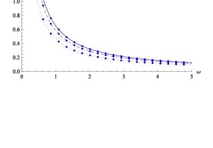
Figure 3.1: The real and imaginary conductivity for $C=0$(solid), $2$(dashed) and $4$(dotted), where we set $2\pi\alpha^{\prime}=1$, $\alpha=-\eta=1$, $\Lambda=-3$, $\tau_{\rm eff}=1$ and $v_{+}=10$.

4 Massive charge carriers

We will consider the effects of massive charge carriers in this section, which are more closely related to model building for real -world strange metals. In this case, the energy gap is large compared to the temperature: $E_{\rm gap}\gg T$. When translated into the language of probe D-branes, the massive charge carriers correspond to flavor branes wrapping internal cycles, whose volumes vary with radial direction [30, 33].

As was pointed out in [30, 33], at finite temperature the flavor brane shrinks to a point at $v=v_{0}$ for large enough mass. In this case the charge carriers correspond to strings stretching from the flavor brane from $v=v_{0}$ to the black hole horizon $v=v_{+}$. In a dilute limit one can consider a small density of such strings and ignore the backreaction. For larger densities the backreaction cannot be neglected and the resulting configuration is that the brane forms a “spike” in place of the strings. We will study the dilute limit first and then take the backreaction into account.

4.1 Conductivity in the dilute regime

The massive charge carriers can be treated as strings stretching from the probe brane to the black hole horizon in the dilute limit, while there are no interactions between the strings. In this limit the probe brane is described by the zero-density solution, which is has a cigar shape with $v=v_{0}$ at the tip.

Let us take the static gauge $t=\tau,v=\sigma$. When expanded to quadratic order for the transverse fluctuations, the Nambu-Goto action

$$S_{\rm NG}=-T\int d\tau d\sigma\sqrt{-{\rm det}h_{ab}}+\int A$$ (4.1)

gives the following field equation

$$-\frac{1}{\alpha^{\prime}}\frac{a^{2}_{0}f(v)}{v^{2a_{1}+2b_{1}-2}}\partial_{v}x^{i}+F_{i0}+F_{ij}\dot{x}^{j}=0.$$ (4.2)

Notice that we have incorporated the surface terms.

In the zero-frequency limit, the field equation can be easily integrated out

$$x^{i}=V^{i}(t+\frac{1}{v_{+}^{2b_{1}}}\int^{v}\frac{u^{2a_{1}+2b_{1}-2}}{a_{0}^{2}f(u)}du),$$ (4.3)

where $V^{i}$ is an integration constant and the relative normalization of the two terms is fixed by imposing incoming boundary conditions at the horizon. By assuming $v_{0}\ll v_{+}$, at the boundary we can obtain

$$\frac{1}{v_{+}^{2b_{1}}}\frac{1}{\alpha^{\prime}}V^{i}=F_{i0}+F_{ij}V^{j},$$ (4.4)

According to Drude’s law we have the following relation

$$\frac{m}{\tau}\propto\frac{1}{\alpha^{\prime}}T^{\frac{2b_{1}}{2a_{1}-1}},$$ (4.5)

Therefore the DC conductivity in the dilute limit of the massive charge carriers is given by

$$\sigma=\frac{\tau}{m}J^{t}\propto\frac{J^{t}}{T^{\frac{2b_{1}}{2a_{1}-1}}}.$$ (4.6)

Next we consider the AC case. Before performing the calculations we shall determine one scale of interest, the energy gap, which corresponds to the mass of the string stretching from $v_{0}$ to $v_{+}$,

$$E_{\rm gap}=\int^{v_{+}}_{v_{0}}dv\sqrt{-g_{tt}g_{vv}}/\alpha^{\prime}=\frac{L^{2}}{\alpha^{\prime}v_{0}},$$ (4.7)

where another natural scale $\omega_{0}=v_{0}^{-1}$ corresponding to the energy scale of bulk excitations at $v_{0}$, is introduced.

The bulk equation of motion for $x(v,t)={\rm Re}(X_{\omega}(v)e^{-i\omega t})$ reads

$$\partial_{v}(\frac{a_{0}^{2}f(v)}{v^{2a_{1}+2b_{1}-2}}\partial_{v}X_{\omega})=-\omega^{2}\frac{v^{2a_{1}-2b_{1}-2}}{a^{2}_{0}f(v)}X_{\omega}.$$ (4.8)

Now consider the case of zero magnetic field $F_{10}=E,F_{ij}=0$, at the boundary $v=v_{0}$ the surface term gives

$$\frac{1}{\alpha^{\prime}}\frac{a^{2}_{0}f(v_{0})}{v^{2a_{1}+2b_{1}-2}_{0}}\partial_{v}X_{\omega}(v_{0})=E.$$ (4.9)

Then the conductivity can be evaluated as

$$\sigma=\frac{J^{t}V_{\omega}(v_{0})}{E}=\frac{i\omega J^{t}X_{\omega}(v_{0})}{E}=\frac{i\omega\alpha^{\prime}J^{t}X_{\omega}(v_{0})v^{2a_{1}+2b_{1}-2}}{a^{2}_{0}f(v_{0})\partial_{\omega}X(v_{0})},$$ (4.10)

Consider the very high frequency limit $\omega\gg\omega_{0}$, in this case the WKB approximation can be adopted in the whole range $v_{0}\leq v\leq v_{+}$. The leading WKB solution is given by

$$X_{\omega}(v)\approx C_{1}e^{-i\int^{v}_{v_{0}}\frac{\omega v^{2a_{1}-2}}{a^{2}_{0}f(v)}}+C_{2}e^{i\int^{v}_{v_{0}}\frac{\omega v^{2a_{1}-2}}{a^{2}_{0}f(v)}}.$$ (4.11)

Then the conductivity in this regime is

$$\partial_{v}X_{\omega}(v_{0})\sim\frac{i\omega v^{2a_{1}-2}_{0}}{a_{0}^{2}f(v_{0})}X_{\omega}(v_{0}),$$ (4.12)

$$\sigma_{\rm WKB}=\alpha^{\prime}L^{-2}J^{t}v^{2b_{1}-2}_{0}.$$ (4.13)

Next we consider the limit $T\ll\omega\ll\omega_{0}$, For $v\ll v_{+}$, we have $f\approx 1$ and the equation of motion turns out to be

$$\partial^{2}_{v}X_{\omega}-(2a_{1}+2b_{1}-2)\frac{1}{v}\partial_{v}X_{\omega}+\frac{\omega^{2}}{a^{4}_{0}}v^{4a_{1}-4}X_{\omega}=0.$$ (4.14)

The solution is given in terms of the Bessel function

$$X_{\omega}(v)=v^{\xi\kappa}\omega^{\xi}H^{(1)}_{\xi}(\frac{\omega v^{\kappa}}{\kappa a^{2}_{0}}),$$ (4.15)

where

$$\kappa=a_{1}-b_{1},\leavevmode\nobreak\ \leavevmode\nobreak\ \leavevmode\nobreak\ \xi=\frac{2a_{1}+2b_{1}-1}{2a_{1}-2b_{1}}.$$ (4.16)

In the regime $\omega\ll E_{\rm gap}$, we can expand the solution for small argument

$$X_{\omega}\propto 1-\frac{1}{\Gamma(-\xi)}(\frac{\omega v^{\kappa}}{2\kappa a^{2}_{0}})^{2}+e^{i\pi\xi}(\frac{\omega v^{\kappa}}{2\kappa a^{2}_{0}})^{2\xi}.$$ (4.17)

The following situations should be discussed separately when evaluating the conductivity. The conductivity is given by the following formula when the second term dominates

$$\sigma=-i\omega^{-1}2\kappa\Gamma(-\xi)\alpha^{\prime}L^{-2}J^{t}a^{2}_{0}v^{4b_{1}-1}_{0},$$ (4.18)

which is a Drude result. When the third term dominates, the conductivity possesses a nontrivial scaling

$$\sigma=\frac{a^{4\xi-2}_{0}}{2\xi}(2\kappa)^{2\xi}\alpha^{\prime}L^{-2}J^{t}e^{i\pi(\frac{1}{2}-\xi)}\omega^{1-2\xi}.$$ (4.19)

In sum, we have the following scaling behaviors for the resistivity and conductivity in the dilute regime,

$$\rho=\frac{1}{\sigma}\sim T^{\frac{2b_{1}}{2b_{1}-2a_{1}}},\leavevmode\nobreak\ \leavevmode\nobreak\ \leavevmode\nobreak\ \sigma(\omega)\sim\omega^{1-2\xi},$$ (4.20)

where $\xi$ is given in (4.16). Notice that in real-world strange metals,

$$\rho\sim T^{\nu_{1}},\leavevmode\nobreak\ \leavevmode\nobreak\ \leavevmode\nobreak\ \sigma(\omega)\sim\omega^{-\nu_{2}},$$ (4.21)

where $\nu_{1}\approx 1,\nu_{2}\approx 0.65$ [36]. Therefore if we require our dual gravitational background to exhibit the same scaling behavior, we have to set

$$\alpha=\pm 0.293491,\leavevmode\nobreak\ \leavevmode\nobreak\ \leavevmode\nobreak\ \eta=\pm 1.45201.$$ (4.22)

The consistency of the above choices for the parameters has been verified.

4.2 Conductivity at finite densities

When the backreaction of the massive charge carriers cannot be neglected, we should introduce an additional scalar field which corresponds to the “mass” operator in the boundary field theory. The volume of the internal cycle wrapped by the probe brane is determined by this scalar field. In this case the DBI action becomes

$$S_{q}=-\tau_{\rm eff}\int dtd^{2}xdvv^{-k_{0}}V(\theta)^{n}\sqrt{g_{xx}}\sqrt{-g_{tt}g_{xx}g_{\sigma\sigma}-(2\pi\alpha^{\prime})^{2}(g_{\sigma\sigma}E^{2}+g_{xx}\Phi^{\prime 2}+g_{tt}h^{\prime 2})},$$ (4.23)

where $V(\theta)^{n}$ denotes the volume of the $n$-dimensional submanifold wrapped by the probe brane. Notice that here we have introduced the worldvolume gauge field as follows

$$A=\Phi(v)dt+(-Et+h(v))dx$$ (4.24)

and the induced metric component is given by $g_{\sigma\sigma}=g_{vv}+\theta^{\prime 2}$.

We can obtain the following constants of motion

$$C=\frac{-g_{xx}^{3/2}\Phi^{\prime}v^{-k_{0}}V(\theta)^{n}}{\sqrt{-g_{tt}g_{xx}g_{\sigma\sigma}-(2\pi\alpha^{\prime})^{2}(g_{\sigma\sigma}E^{2}+g_{xx}\Phi^{\prime 2}+g_{tt}h^{\prime 2})}},$$ (4.25)

$$H=\frac{-g_{tt}g_{xx}^{1/2}h^{\prime}v^{-k_{0}}V(\theta)^{n}}{\sqrt{-g_{tt}g_{xx}g_{\sigma\sigma}-(2\pi\alpha^{\prime})^{2}(g_{\sigma\sigma}E^{2}+g_{xx}\Phi^{\prime 2}+g_{tt}h^{\prime 2})}}.$$ (4.26)

Therefore the on-shell DBI action turns out to be

$$S_{q}=-\tau_{\rm eff}\int dtd^{2}xdvv^{-2k_{0}}V(\theta)^{2n}g_{xx}^{3/2}\sqrt{-g_{tt}g_{\sigma\sigma}}GF^{1/2},$$ (4.27)

where

$$GF=\frac{g_{tt}g_{xx}+(2\pi\alpha^{\prime})^{2}E^{2}}{(2\pi\alpha^{\prime})^{2}(C^{2}g_{tt}+H^{2}g_{xx})+g^{2}_{xx}g_{tt}v^{-2k_{0}}V(\theta)^{2n}}.$$ (4.28)

The background profile of the probe brane $\theta(v)$ is determined by

$$\frac{d}{dv}[v^{-2k_{0}}V(\theta)^{2n}g^{3/2}_{xx}\sqrt{\frac{-g_{tt}}{g_{\sigma\sigma}}}\theta^{\prime}GF^{1/2}]-\frac{d}{d\theta}[v^{-2k_{0}}V(\theta)^{2n}g^{3/2}_{xx}\sqrt{-g_{tt}g_{\sigma\sigma}}GF^{1/2}]=0.$$ (4.29)

Finally, following the same steps straightforwardly, we obtain the DC conductivity

$$\sigma=\sqrt{(2\pi\alpha^{\prime})^{4}\tau_{\rm eff}^{2}v^{-2k_{0}}_{\ast}V(\theta_{\ast})^{2n}+(\frac{2\pi\alpha^{\prime}}{L^{2}})^{2}(J^{t})^{2}v^{4b_{1}}_{\ast}}.$$ (4.30)

Note that in the massless limit $V(\theta)\leavevmode\nobreak\ \rightarrow\leavevmode\nobreak\ 1$, the above result reduces to the one obtained in previous section (3.18).

The calculations of the AC conductivity are similar to the massless case, that is, we will study the Maxwell fluctuations up to quadratic order and consider zero momentum $k=0$. One crucial difference is that here we have non-trivial background profile $\theta(v)$. The linearized equation for the longitudinal fluctuation is given by

$$\partial_{v}(v^{-k_{0}}V(\theta)^{n}\gamma\sqrt{\frac{-g_{tt}}{g_{\sigma\sigma}}}A_{x}^{\prime})=-v^{-k_{0}}V(\theta)^{n}\gamma\sqrt{\frac{g_{\sigma\sigma}}{-g_{tt}}}\omega^{2}A_{x},$$ (4.31)

where

$$\gamma\equiv\sqrt{1+(2\pi\alpha^{\prime})^{2}\frac{C^{2}v^{2k_{0}+4b_{1}}}{V(\theta)^{2n}}}.$$ (4.32)

The equation for the fluctuation can still be transformed into a Schrödinger form. After defining

$$A_{x}=(v^{-k_{0}}V(\theta)^{n}\gamma)^{-1/2}\Psi,\leavevmode\nobreak\ \leavevmode\nobreak\ \leavevmode\nobreak\ \frac{d}{dv}=\sqrt{\frac{g_{\sigma\sigma}}{-g_{tt}}}\frac{d}{ds},$$ (4.33)

(4.31) becomes

$$-\frac{d^{2}}{ds^{2}}\Psi+U\Psi=\omega^{2}\Psi,$$ (4.34)

with the following effective potential

$$U=\frac{1}{2}\frac{1}{\sqrt{v^{-k_{0}}V(\theta)^{n}\gamma}}\frac{d}{ds}[\frac{1}{\sqrt{v^{-k_{0}}V(\theta)^{n}\gamma}}\frac{d}{ds}(v^{-k_{0}}V(\theta)^{n}\gamma)].$$ (4.35)

At first sight one may consider that we can perform similar calculations as for the massless case. However, one key point in the calculations of [15] was that in a wide range $v_{0}<v<v_{+}$, the profile of the embedding was approximately constant. This behavior was confirmed by numerical calculations and played a crucial role in simplifying the corresponding Schrödinger equation. Unfortunately, here we cannot find such a constant behavior for the profile of the embedding. The profile turns out to be singular in the near horizon region. Thus we cannot simplify the Schrödinger equation considerably to find the analytic solutions. It might be related to the non-trivial dilaton field in the DBI action and we expect that such singular behavior may be cured in realistic D-brane configurations, which might enable us to calculate the transport coefficients.

5 Summary and discussion

The holographic model building of “strange” metals was initiated in [15], where the authors considered Lifshitz black holes as the background and probe D-branes as charge carriers. In this paper we generalize the analysis to backgrounds with anisotropic scaling symmetry, which are solutions of the Einstein-Maxwell-dilaton theory coupled with a Liouville potential. For massless charge carriers, we obtain the DC conductivity and DC Hall conductivity by applying the approach proposed in [31] and [32]. The results can reproduce those obtained in [15] in certain specific limits. We also calculate the AC conductivity by transforming the corresponding equation of motion into the Schrödinger equation. For massive charge carriers, the DC and AC conductivities are also obtained in the dilute limit. When the dual gravity background exhibits the scaling behaviors for strange metals, the parameters in the action should take the following values, $\alpha=\pm 0.293491$ and $\eta=\pm 1.45201$. We also obtain the DC conductivity at finite density. One thing we are not able to analyze is the AC conductivity at finite density, which may be due to the singular behavior of the profile of the brane embedding. We expect that such a difficulty may be cured in realistic D-brane configurations.

In the final stage of this work we noticed that some overlaps appeared in [27]. They clarified the landscape of effective holographic theories in view of condensed matter applications by studying the thermodynamics, spectra and conductivities of several classes of charged dilatonic black hole solutions that include the charge density backreaction fully. In particular, they obtained the DC and AC conductivities in the context of the DBI action. It should be pointed out that one crucial difference is that we consider the solution as the global solution, while they imposed some constraints to ensure that the solutions were asymptotically AdS. Another topic which was not included in their paper is the DC Hall conductivity. However, we believe that our results are consistent with theirs.

One important further direction is to study the fermionic nature of the dual gravity background, as Fermi surfaces and other related observables are crucial for the description of strange metals. One may perform the analysis along the line of [37, 38, 39, 40]. One point is that in those papers the asymptotic geometry was AdS_d+2 and the near horizon geometry contained an AdS₂ part, which played a central role in the investigations. Although the asymptotic and/or near horizon geometries possess anisotropic scaling symmetry, it is believed that similar analysis can be performed by making use of the “matching” technique adopted in the above mentioned references. Furthermore, one may examine the fermionic correlators in the background studied in this paper, following [41, 42, 43]. We expect to study such interesting problems in the future.

Acknowledgements

DWP would like to thank Andy O’Bannon for helpful discussions. This work was supported by the National Research Foundation of Korea(NRF) grant funded by the Korea government(MEST) through the Center for Quantum Spacetime(CQUeST) of Sogang University with grant number 2005-0049409.

References

-
[1]
J. M. Maldacena,
“The large N limit of superconformal field theories and supergravity,”
Adv. Theor. Math. Phys. 2, 231 (1998)
[Int. J. Theor. Phys. 38, 1113 (1999)]
[arXiv:hep-th/9711200].
S. S. Gubser, I. R. Klebanov and A. M. Polyakov, “Gauge theory correlators from non-critical string theory,” Phys. Lett. B 428, 105 (1998) [arXiv:hep-th/9802109].
E. Witten, “Anti-de Sitter space and holography,” Adv. Theor. Math. Phys. 2, 253 (1998) [arXiv:hep-th/9802150]. - [2] O. Aharony, S. S. Gubser, J. M. Maldacena, H. Ooguri and Y. Oz, “Large N field theories, string theory and gravity,” Phys. Rept. 323, 183 (2000) [arXiv:hep-th/9905111].
-
[3]
S. A. Hartnoll,
“Lectures on holographic methods for condensed matter physics,”
Class. Quant. Grav. 26, 224002 (2009)
[arXiv:0903.3246 [hep-th]].
C. P. Herzog, “Lectures on Holographic Superfluidity and Superconductivity,” J. Phys. A 42, 343001 (2009) [arXiv:0904.1975 [hep-th]].
J. McGreevy, “Holographic duality with a view toward many-body physics,” arXiv:0909.0518 [hep-th].
G. T. Horowitz, “Introduction to Holographic Superconductors,” arXiv:1002.1722 [hep-th].
S. Sachdev, “Condensed matter and AdS/CFT,” arXiv:1002.2947 [hep-th]. - [4] S. S. Gubser, “Breaking an Abelian gauge symmetry near a black hole horizon,” Phys. Rev. D 78, 065034 (2008) [arXiv:0801.2977 [hep-th]].
- [5] S. A. Hartnoll, C. P. Herzog and G. T. Horowitz, “Building a Holographic Superconductor,” Phys. Rev. Lett. 101, 031601 (2008) [arXiv:0803.3295 [hep-th]].
- [6] S. S. Gubser and S. S. Pufu, “The gravity dual of a p-wave superconductor,” JHEP 0811, 033 (2008) [arXiv:0805.2960 [hep-th]].
- [7] S. A. Hartnoll, C. P. Herzog and G. T. Horowitz, “Holographic Superconductors,” JHEP 0812, 015 (2008) [arXiv:0810.1563 [hep-th]].
- [8] J. W. Chen, Y. J. Kao, D. Maity, W. Y. Wen and C. P. Yeh, “Towards A Holographic Model of D-Wave Superconductors,” Phys. Rev. D 81, 106008 (2010) [arXiv:1003.2991 [hep-th]].
- [9] C. P. Herzog, “An Analytic Holographic Superconductor,” arXiv:1003.3278 [hep-th].
- [10] M. Ammon, J. Erdmenger, M. Kaminski and P. Kerner, “Superconductivity from gauge/gravity duality with flavor,” Phys. Lett. B 680, 516 (2009) [arXiv:0810.2316 [hep-th]].
- [11] M. Ammon, J. Erdmenger, M. Kaminski and P. Kerner, “Flavor Superconductivity from Gauge/Gravity Duality,” JHEP 0910, 067 (2009) [arXiv:0903.1864 [hep-th]].
- [12] S. S. Gubser, C. P. Herzog, S. S. Pufu and T. Tesileanu, “Superconductors from Superstrings,” Phys. Rev. Lett. 103, 141601 (2009) [arXiv:0907.3510 [hep-th]].
- [13] J. P. Gauntlett, J. Sonner and T. Wiseman, “Holographic superconductivity in M-Theory,” Phys. Rev. Lett. 103, 151601 (2009) [arXiv:0907.3796 [hep-th]].
- [14] M. Kaminski, “Flavor Superconductivity and Superfluidity,” arXiv:1002.4886 [hep-th].
- [15] S. A. Hartnoll, J. Polchinski, E. Silverstein and D. Tong, “Towards strange metallic holography,” JHEP 1004, 120 (2010) [arXiv:0912.1061 [hep-th]].
- [16] G. W. Gibbons and K. i. Maeda, “Black Holes And Membranes In Higher Dimensional Theories With Dilaton Fields,” Nucl. Phys. B 298, 741 (1988).
- [17] J. Preskill, P. Schwarz, A. D. Shapere, S. Trivedi and F. Wilczek, “Limitations on the statistical description of black holes,” Mod. Phys. Lett. A 6, 2353 (1991).
- [18] D. Garfinkle, G. T. Horowitz and A. Strominger, “Charged black holes in string theory,” Phys. Rev. D 43, 3140 (1991) [Erratum-ibid. D 45, 3888 (1992)].
- [19] C. F. E. Holzhey and F. Wilczek, “Black holes as elementary particles,” Nucl. Phys. B 380, 447 (1992) [arXiv:hep-th/9202014].
- [20] K. Goldstein, S. Kachru, S. Prakash and S. P. Trivedi, “Holography of Charged Dilaton Black Holes,” arXiv:0911.3586 [hep-th].
- [21] S. Kachru, X. Liu and M. Mulligan, “Gravity Duals of Lifshitz-like Fixed Points,” Phys. Rev. D 78, 106005 (2008) [arXiv:0808.1725 [hep-th]].
- [22] M. Taylor, “Non-relativistic holography,” arXiv:0812.0530 [hep-th].
- [23] S. S. Gubser and F. D. Rocha, “Peculiar properties of a charged dilatonic black hole in ,” Phys. Rev. D 81, 046001 (2010) [arXiv:0911.2898 [hep-th]].
- [24] J. Gauntlett, J. Sonner and T. Wiseman, “Quantum Criticality and Holographic Superconductors in M-theory,” JHEP 1002, 060 (2010) [arXiv:0912.0512 [hep-th]].
- [25] M. Cadoni, G. D’Appollonio and P. Pani, “Phase transitions between Reissner-Nordstrom and dilatonic black holes in 4D AdS spacetime,” arXiv:0912.3520 [hep-th].
- [26] C. M. Chen and D. W. Pang, “Holography of Charged Dilaton Black Holes in General Dimensions,” arXiv:1003.5064 [hep-th].
- [27] C. Charmousis, B. Gouteraux, B. S. Kim, E. Kiritsis and R. Meyer, “Effective Holographic Theories for low-temperature condensed matter systems,” arXiv:1005.4690 [hep-th].
-
[28]
R. G. Cai and Y. Z. Zhang,
“Black plane solutions in four-dimensional spacetimes,”
Phys. Rev. D 54, 4891 (1996)
[arXiv:gr-qc/9609065].
R. G. Cai, J. Y. Ji and K. S. Soh, “Topological dilaton black holes,” Phys. Rev. D 57, 6547 (1998) [arXiv:gr-qc/9708063].
C. Charmousis, B. Gouteraux and J. Soda, “Einstein-Maxwell-Dilaton theories with a Liouville potential,” Phys. Rev. D 80, 024028 (2009) [arXiv:0905.3337 [gr-qc]]. - [29] B. H. Lee, S. Nam, D. W. Pang and C. Park, “Conductivity in the anisotropic background,” arXiv: 1006.0779 [hep-th].
- [30] A. Karch and E. Katz, “Adding flavor to AdS/CFT,” JHEP 0206, 043 (2002) [arXiv:hep-th/0205236].
- [31] A. Karch and A. O’Bannon, “Metallic AdS/CFT,” JHEP 0709, 024 (2007) [arXiv:0705.3870 [hep-th]].
- [32] A. O’Bannon, “Hall Conductivity of Flavor Fields from AdS/CFT,” Phys. Rev. D 76, 086007 (2007) [arXiv:0708.1994 [hep-th]].
- [33] S. Kobayashi, D. Mateos, S. Matsuura, R. C. Myers and R. M. Thomson, “Holographic phase transitions at finite baryon density,” JHEP 0702, 016 (2007) [arXiv:hep-th/0611099].
- [34] S. S. Gubser and F. D. Rocha, “The gravity dual to a quantum critical point with spontaneous symmetry breaking,” Phys. Rev. Lett. 102, 061601 (2009) [arXiv:0807.1737 [hep-th]].
- [35] G. T. Horowitz and M. M. Roberts, “Zero Temperature Limit of Holographic Superconductors,” JHEP 0911, 015 (2009) [arXiv:0908.3677 [hep-th]].
- [36] D. van de Marel et al., “Quantum critical behaviour in a high-tc superconductor,” Nature 425 (2003) 271.
- [37] S. S. Lee, “A Non-Fermi Liquid from a Charged Black Hole: A Critical Fermi Ball,” Phys. Rev. D 79, 086006 (2009) [arXiv:0809.3402 [hep-th]].
- [38] H. Liu, J. McGreevy and D. Vegh, “Non-Fermi liquids from holography,” arXiv:0903.2477 [hep-th].
- [39] M. Cubrovic, J. Zaanen and K. Schalm, “String Theory, Quantum Phase Transitions and the Emergent Fermi-Liquid,” Science 325, 439 (2009) [arXiv:0904.1993 [hep-th]].
- [40] T. Faulkner, H. Liu, J. McGreevy and D. Vegh, “Emergent quantum criticality, Fermi surfaces, and AdS2,” arXiv:0907.2694 [hep-th].
- [41] S. S. Gubser, F. D. Rocha and P. Talavera, “Normalizable fermion modes in a holographic superconductor,” arXiv:0911.3632 [hep-th].
- [42] T. Faulkner, G. T. Horowitz, J. McGreevy, M. M. Roberts and D. Vegh, “Photoemission ’experiments’ on holographic superconductors,” JHEP 1003, 121 (2010) [arXiv:0911.3402 [hep-th]].
- [43] T. Faulkner, N. Iqbal, H. Liu, J. McGreevy and D. Vegh, “From black holes to strange metals,” arXiv:1003.1728 [hep-th].